Parametric coupling between macroscopic quantum resonators

Abstract

Time-dependent linear coupling between macroscopic quantum resonator modes generates both a parametric amplification also known as a “squeezing operation” and a beam splitter operation, analogous to quantum optical systems. These operations, when applied properly, can robustly generate entanglement and squeezing for the quantum resonator modes. Here, we present such coupling schemes between a nanomechanical resonator and a superconducting electrical resonator using applied microwave voltages as well as between two superconducting lumped-element electrical resonators using a r.f. SQUID-mediated tunable coupler. By calculating the logarithmic negativity of the partially transposed density matrix, we quantitatively study the entanglement generated at finite temperatures. We also show that characterization of the nanomechanical resonator state after the quantum operations can be achieved by detecting the electrical resonator only. Thus, one of the electrical resonator modes can act as a probe to measure the entanglement of the coupled systems and the degree of squeezing for the other resonator mode.

1 Introduction

The quantum behavior of macroscopic resonators has only recently been demonstrated in solid-state systems and is currently under intensive exploration. Electrical resonators such as a superconducting transmission line resonator coupled to a single Cooper pair box or phase qubits and a d.c. SQUID resonator interacting with a flux qubit have shown features of single microwave quanta [1, 2, 3, 4]. Nanomechanical resonators capacitively coupled to a single electron transistor have been measured, approaching the quantum limit with femtometer displacements [5, 6, 7, 8]. Recently, a transmission line resonator coupled to a nanomechanical resonator has been used to cool the nanomechanical motion to hundreds of quanta [9]. Besides being a wonderful testing ground for exploring quantum physics at the macroscopic level, these systems can provide high-Q harmonic-oscillator networks for quantum engineering and quantum information processing [10].

Micro-fabricated resonators interact by electromagnetic forces. By controlling the circuit parameters, various time-dependent couplings can be generated to manipulate the quantum state of the coupled system. In a previous work [11], one of us (L.T.) studied the effective amplification of the coupling amplitude between a nanomechanical resonator and a qubit by parametrically pumping the qubit with a fast pulse. This scheme can be applied to produce entanglement between resonator modes as well as to generate Schrödinger cat states in the nanomechanical system. In a recent work [12], it was shown that by controlling the coupling between a nanomechanical resonator and an ancilla qubit, it is possible to engineer an arbitrary Hamiltonian for the nanomechanical resonator mode. In another work [13], a pulse technique is used to form arbitrary quantum states of a nanomechanical resonator in the coupled resonator-qubit system. In addition, experimental realization of parametric coupling has been achieved for two coupled flux qubits [14].

In this paper, we show that quantum features such as entanglement and squeezing can be generated and tested using the Gaussian states of macroscopic resonator modes coupled in a tunable way. Parametric modulation of the coupling strength results in a squeezing operation or a beam splitter operation, necessary ingredients for engineering quantum features. Starting from a separable initial state, inseparability (or entanglement) can be generated by linear operations. Two physical systems are studied: in one system a nanomechanical resonator is capacitively coupled to a superconducting electrical resonator mode, in another system two lumped-element electrical resonators are coupled to each other through a tunable mutual inductance. In the first system, if we start with both the nanomechanical and electrical resonator modes in their ground states, careful control over squeezing and beam splitter operations can produce squeezed states in the nanomechanical mode. Note that previous work on creating squeezed states [15] in nanomechanical-resonator systems uses quantum reservoir engineering, feedback control techniques, and an (effective) nonlinear coupling [16, 17, 18, 19]. One advantage of the scheme described here is that linear coupling between the solid-state resonators, realizable with current technology, can be easily controlled in both magnitude and frequency. In addition, our approach not only provides a method for generating entanglement and squeezed states, but it also provides a practical way for detecting the squeezing. We show that for Gaussian states, complete information about the coupled resonators can be obtained by only measuring the quadrature variances of the electrical resonator mode [22] which couples more strongly to the detector than the mechanical mode. In this way, we can avoid any difficulties associated with directly measuring the nanomechanical mode with high resolution. Here, the electrical resonator plays the role of a knob that controls the behavior of the nanomechanical resonator while also acting as a detector to probe this behavior. Using a r.f. SQUID-mediated tunable coupler, this work can be extended in a straightforward way to a system with two coupled electrical resonator modes. For typical dilution refrigerator temperatures ($\sim 30$ mK), we can pick both resonator frequencies ($\sim 10$ GHz) to operate above the quantum limit where the two electrical resonators will definitely be cooled to their ground state, making it easy to prepare these modes in squeezed states by linear operations. Also, the two modes can be measured simultaneously, which provides a direct observation of the cross correlations between the two modes for a clear comparison with theoretical predictions.

Entanglement is the key component for many quantum information protocols such as quantum teleportation. Previous work [23] studied the quantum teleportation of nanomechanical modes in a purely solid-state network, where high fidelity could be achieved for the final state with the assistance of a highly entangled two-mode squeezed vacuum state even at finite resonator temperatures. The schemes studied in this paper provide a detailed account of how to engineer and evaluate this entanglement to ensure the success of the quantum teleportation protocol, as well as to generate one important quantum state – a squeezed state of the resonators.

2 Coupled macroscopic resonators

In this section, we investigate the realization of linear, tunable coupling between macroscopic resonator modes and the parametric modulation of such coupling using a circuit architecture.

2.1 a nanomechanical mode coupled to transmission line resonator

First, consider a nanomechanical resonator capacitively coupled to a resonant superconducting transmission line. Quantum behavior of high-Q electrical modes has been demonstrated using superconducting transmission lines [5]. The eigenmodes of a one dimensional transmission line resonator of length $L$ between $(-L/2,L/2)$ can be obtained by considering the charge distribution along the transmission line,

$$\theta(x,t)=\int_{-L/2}^{x}dx^{\prime}q(x^{\prime},t)$$

where $q(x^{\prime},t)$ is the linear charge density at the location $x$. The lowest even mode has the voltage distribution

$$V(x)=\frac{1}{c}\frac{\partial\theta}{\partial x}=\sqrt{\frac{\hbar\omega_{b}}{cL}}\cos\frac{2\pi x}{L}\left(\hat{b}+\hat{b}^{\dagger}\right)$$ (1)

after the quantization of the variables. Here, the frequency of this mode is $\omega_{b}=2\pi/L\sqrt{lc}$, with $l$ the inductance per unit length and $c$ the capacitance per unit length of the transmission line.

The nanomechanical resonator is located at the middle of the superconducting transmission line near $x=0$ which is a voltage antinote of this even mode (figure 1). The nanomechanical resonator is coupled capacitively via a displacement dependent capacitance $C_{x}$. To lowest order, $C_{x}=C_{x}^{0}(1+\hat{x}_{a}/d_{0})$ depends linearly on the displacement coordinate of the nanomechanical motion. The coupled interaction can be derived as

$$H_{int}=\frac{1}{2}C_{x}^{0}(1+\frac{\hat{x}}{d_{0}})(V_{x}-V(0))^{2}$$ (2)

where the nanomechanical resonator is biased at $V_{x}$ and $d_{0}$ is an effective distance between the two resonator electrodes. We study the behavior of the lowest nanomechanical mode with a displacement $\hat{x}=\delta x_{0}(\hat{a}+\hat{a}^{\dagger})$, where $\omega_{a}$ is the frequency of the mechanical mode, $m$ is the effective mass and $\delta x_{0}=\sqrt{\hbar/2m\omega_{a}}$. The interaction can be derived as $H_{int}=-\frac{\hat{x}}{d_{0}}C_{x}^{0}V_{x}V(0)$, assuming that the size of the nanomechanical resonator is much smaller than the length of the transmission line. If we apply a voltage $V_{x}(t)=2V_{x}^{0}\sin\omega_{d}t$ with a drive frequency $\omega_{d}$, the linear interaction can be written as $H_{int}=-2\lambda_{0}\sin\omega_{d}t(\hat{a}+\hat{a}^{\dagger})(\hat{b}+\hat{b}^{\dagger})$ with a coupling strength

$$\lambda_{0}=C_{x}^{0}V_{x}^{0}\frac{\delta x_{0}}{d_{0}}\sqrt{\frac{\hbar\omega_{b}}{cL}}$$ (3)

By adjusting the driving frequency of the voltage, it is possible to generate various linear operations, as discussed in more detail in section 3. Hence, the modulation of the coupling strength provides an effective tool for controlling the entanglement of the coupled resonators.

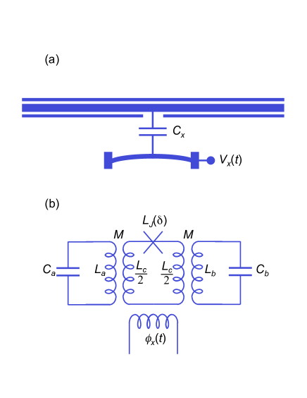
Figure 1: (a) A nanomechanical resonator interacts via a capacitance $C_{x}$ with a transmission line resonator. (b) Two lumped-element electrical resonators interact via a r.f SQUID-mediated tunable coupler.

2.2 two coupled lumped-element resonator modes

Alternatively, two electrical resonators can be coupled together using a r.f. SQUID-mediated tunable coupler. The circuit schematic (figure 1) shows a r.f. SQUID placed between two lumped-element $LC$-resonators. The r.f. SQUID acts like an inductive transformer where the Josephson junction provides a tunable inductance $L_{J}(\delta)=\Phi_{0}/(2\pi I_{o}cos(\delta))$ and $\delta$ is the phase difference across the junction, $I_{o}$ is the junction critical current, and $\Phi_{0}$ is a flux quantum. The use of small Josephson junctions with high current density allows us to ignore the self capacitance $C_{J}$ of the junction so that we remain in an operation regime where $\omega^{2}L_{J}C_{J}\ll 1$ for all the relevant frequencies $\omega$. Furthermore, by careful design and operation, we can avoid any direct coupling between the two resonators so that a single effective mutual inductance,

$$M_{eff}(\delta)=\frac{M^{2}}{L_{c}+L_{J}(\delta)}$$ (4)

derives only from the mutual inductive coupling $M$ between each resonator and the central r.f. SQUID transformer coil with geometrical self inductance $L_{c}$. This leads to a coupled interaction of strength [24],

$$H_{int}(\delta)=-M_{eff}(\delta)\sqrt{\frac{\hbar\omega_{a}}{2L_{a}}\frac{\hbar\omega_{b}}{2L_{b}}}(\hat{a}+\hat{a}^{\dagger})(\hat{b}+\hat{b}^{\dagger}),$$ (5)

where $\omega_{a}$ and $\omega_{b}$ are frequencies of the two resonators respectively.

In order to modulate the coupling between the resonators, we must modulate the phase difference $\delta$. This can be achieved using a r.f. bias coil which applies an external flux $\phi_{x}=2\pi\Phi_{x}/\Phi_{o}$ to the r.f. SQUID coil, thereby inducing a current through the Josephson junction and thus changing the phase difference $\delta$. The phase difference $\delta$ is related to the external flux $\phi_{x}$ through flux quantization such that $\beta\sin(\delta)+\delta-\phi_{x}=0$, where $\beta=L_{c}/L_{J}(0)$. This places some constraints on the design and subsequent operation of the tunable coupler [24]. Namely, we would like to operate in a regime where $\beta\lesssim 1$ so that the relationship between $\delta$ and $\phi_{x}$ remains non-hysteretic and the inductive coupling passes from anti-ferromagnetic (AF) through zero to ferromagnetic (FM). If we choose a particular d.c. flux offset and a relatively small amplitude for the r.f. flux modulation, we can achieve a roughly linear relationship between the drive flux $\phi_{x}$ and the effective mutual inductance $M_{eff}$ without any residual direct coupling. An example is shown (figure 2) for $\beta=0.85$ and other device parameters specified later. Thus, for a sinusoidal flux drive $\phi_{x}(t)=\phi_{dc}-\phi_{rf}\sin(\omega_{d}t)$ at frequency $\omega_{d}$, we can produce a sufficient parametric modulation of the coupling strength (5) and hence perform the squeezing or beam splitter operations. With $\phi_{dc}=2.4178$ and $\phi_{rf}=0.0540$, we can closely approximate a sinusoidal variation in the size of the effective mutual inductance (figure 2). Slight deviations from the ideal behavior will only appear as negligibly small residual direct coupling or small amplitude components at higher harmonic frequencies which do not corrupt the squeezing or beam splitter operations.

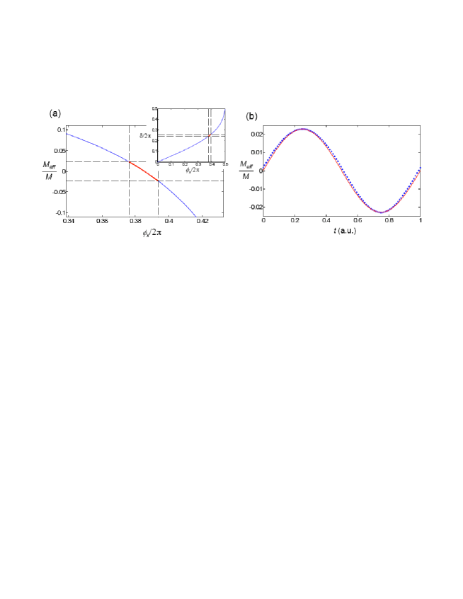
Figure 2: (a) $M_{eff}/M$ versus external $\phi_{x}/2\pi$, where the (red online) highlight is the region where the coupling is modulated. The inset shows the dependence of $\delta$ on $\phi_{x}$ for $\beta=0.85$ (b) $M_{eff}/M$ (points) versus time. The thin (red online) line is a sine function.

A coupling magnitude similar to (3) can be derived for this circuit with

$$\lambda_{0}=\frac{\Delta M_{eff}}{2}\sqrt{\frac{\hbar\omega_{a}}{2L_{a}}\frac{\hbar\omega_{b}}{2L_{b}}}$$ (6)

where $\Delta M_{eff}$ is the amplitude of the modulating effective mutual inductance.

Coupling electrical resonators has several advantages: 1) the coupling between the electrical resonators can be made stronger fairly easily through simple design modifications, more so than for coupling between a mechanical resonator and an electrical resonator, 2) the requirements on device temperature for clearly operating in the quantum regime have also been achieved [1, 2, 3], 3) electrical resonators have already demonstrated sufficiently (high Q’s) long coherence times [1, 2, 3], making is possible to study their dynamic behavior, and 4) direct measurement of both resonators provides more information on the overall quantum behavior of the coupled system. Thus, even if pursuing the nanomechanical approach proves to be difficult, it will be very promising to pursue coupled electrical resonators in order to investigate the generation of entanglement and other quantum physics.

3 Linear operations by parametric coupling

3.1 coupling in the rotating frame

Consider the time-dependent linear coupling between two resonator modes of the form $H_{int}=-2\lambda_{0}\sin\omega_{d}t(\hat{a}+\hat{a}^{\dagger})(\hat{b}+\hat{b}^{\dagger})$, where $\lambda_{0}$ is the coupling amplitude and $\omega_{d}$ is the modulation frequency of the coupling strength. Here the operators $\hat{a}$ ($\hat{a}^{\dagger}$) and $\hat{b}$ ($\hat{b}^{\dagger}$) are the annihilation (creation) operators for the resonant mode. At the driving frequency $\omega_{d}=\omega_{b}-\omega_{a}$, the coupling in the interaction picture has the form

$$H_{I}=i\lambda_{0}(\hat{a}^{\dagger}\hat{b}-\hat{a}\hat{b}^{\dagger})$$ (7)

which generates a beam splitter operation in a similar to fashion to that found in quantum optics. At the driving frequency $\omega_{d}=\omega_{b}+\omega_{a}$, the coupling has the form

$$H_{I}=i\lambda_{0}(\hat{a}\hat{b}-\hat{a}^{\dagger}\hat{b}^{\dagger})$$ (8)

which generates a squeezing operation and hence entanglement between the two modes. These two operations are sufficient for manipulating entanglement and for generating squeezed states of the resonators [20] as we will discuss in detail below.

We focus on the Gaussian states of the coupled resonator modes. A Gaussian state can be fully characterized by the covariance matrix:

$$(\sigma)_{ij}=\frac{1}{2}\langle\hat{x}_{i}\hat{x}_{j}+\hat{x}_{j}\hat{x}_{i}\rangle-[\hat{x}_{i},\hat{x}_{j}]$$ (9)

with $i,j=1,2,3,4$. The operators in this expression are the quadrature variables of the resonators with $\hat{x}_{1}=\hat{x}_{a},\hat{x}_{2}=\hat{p}_{a},\hat{x}_{3}=\hat{x}_{b},\hat{x}_{4}=\hat{p}_{b}$ for the modes $a$ and $b$ respectively. Here $\langle\rangle$ is the ensemble average for the density matrix of the Gaussian states and $[,]$ is the commutator between the variables. Note that linear operations and dissipation due to white noise maps Gaussian states to Gaussian states [25].

The generic form of the covariance matrix for coupled resonators is

$$\sigma=\left(\begin{array}[]{cc}A&C\\ C^{T}&B\end{array}\right)$$ (10)

where $A$ ($B,C$) is $2\times 2$ diagonal matrix with the elements $a_{1}$ and $a_{2}$,

$$A=\left(\begin{array}[]{cc}a_{1}&0\\ 0&a_{2}\end{array}\right)$$ (11)

(and similarly for $b_{i}$ and $c_{i}$). We set the linear displacement to be $\langle\hat{x}_{i}\rangle=0$, which does not affect the entanglement of the system. To describe the finite temperature of the resonators, we use the effective temperature index $\Theta_{\alpha}=\coth\frac{\hbar\omega_{\alpha}}{k_{B}T}$ for $\alpha=a,b$. When $k_{B}T\ll\hbar\omega_{\alpha}$, we have $\Theta_{\alpha}=1$ and the mode is in its ground state. The initial covariance matrix of the thermal states for the uncoupled resonators is a diagonal matrix $\sigma_{0}$ with the diagonal elements $(\Theta_{a},\Theta_{a},\Theta_{b},\Theta_{b})/4$ where the quadrature variances of the resonators are $\langle x_{i}^{2}\rangle=\langle p_{i}^{2}\rangle=\Theta_{i}/4$.

3.2 linear operations: squeezing and beam splitter

It can be shown that the squeezing operation in (8) performs the following transformation on the covariance matrix,

$$\sigma=e^{A_{sq}r_{2}}\sigma_{0}e^{A_{sq}r_{2}}$$ (12)

where

$$A_{sq}=\left(\begin{array}[]{cccc}0&0&1&0\\ 0&0&0&-1\\ 1&0&0&0\\ 0&-1&0&0\end{array}\right)$$

is the squeezing operator and $r_{2}=\lambda_{0}t$ is the squeezing parameter over a duration $t$. We find that

$$e^{A_{sq}r_{2}}=\left(\begin{array}[]{cccc}\cosh r_{2}&0&\sinh r_{2}&0\\ 0&\cosh r_{2}&0&-\sinh r_{2}\\ \sinh r_{2}&0&\cosh r_{2}&0\\ 0&-\sinh r_{2}&0&\cosh r_{2}\end{array}\right).$$

Another linear operation, the beam splitter type of operation, on the resonator modes in (8), performs the following transformation on the covariance matrix,

$$\sigma(\varphi)=e^{A_{bm}^{T}\varphi}\sigma_{0}e^{A_{bm}\varphi}$$ (13)

where $\varphi=\lambda_{0}t$ and

$$A_{bm}=\left(\begin{array}[]{cccc}0&0&1&0\\ 0&0&0&1\\ -1&0&0&0\\ 0&-1&0&0\end{array}\right).$$

We can show that

$$e^{A_{bm}\varphi}=\left(\begin{array}[]{cccc}\cos\varphi&0&-\sin\varphi&0\\ 0&\cos\varphi&0&-\sin\varphi\\ \sin\varphi&0&\cos\varphi&0\\ 0&\sin\varphi&0&\cos\varphi\end{array}\right).$$

This transformation produces a beam splitter operation on the coupled resonators. In particular, it swaps the states of the two modes when $\phi=\pi/2$.

4 Entanglement and squeezing of the coupled resonators

In this section, we study the quantum engineering of entanglement between coupled macroscopic resonator modes and the squeezing of the resonators using the parametric coupling circuits discussed in the previous sections.

4.1 entanglement

At zero temperature, the squeezing operation in (8) generates squeezed vacuum states between two resonator modes which are also entangled states [26]. Here, we show that even at finite temperatures, entanglement can be generated by the squeezing operation starting from an initial state with the covariance matrix $\sigma_{0}$. After a duration $t_{sq}$ with the coupling magnitude $\lambda_{0}$, the squeezing operation transforms the elements of the covariance matrix to

$$a_{1}=a_{2} = \frac{1}{4}\left(\Theta_{a}\cosh^{2}\lambda_{0}t_{sq}+\Theta_{b}\sinh^{2}\lambda_{0}t_{sq}\right)$$

$$b_{1}=b_{2} = \frac{1}{4}\left(\Theta_{a}\sinh^{2}\lambda_{0}t_{sq}+\Theta_{b}\cosh^{2}\lambda_{0}t_{sq}\right)$$ (14)

$$c_{1}=-c_{2} = \frac{1}{4}\left(\Theta_{a}+\Theta_{b}\right)\sinh\lambda_{0}t_{sq}\cosh\lambda_{0}t_{sq}$$

which increase with the squeezing parameter $r_{2}=\lambda_{0}t_{sq}$. Note that the above relation shows $c_{i}\leq\sqrt{a_{i}b_{i}}$ for $i=1,2$ with the equality valid for a large squeezing parameter $r_{2}$.

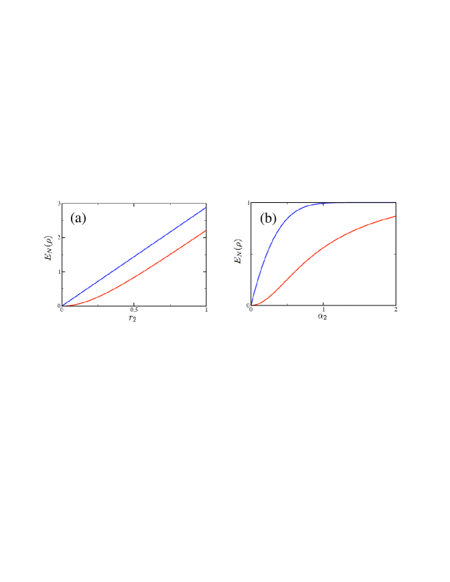
Figure 3: (a) The logarithmic negativity $E_{N}(\rho)$ for the two mode squeezed states versus the squeezing parameter. (b) The logarithmic negativity $E_{N}(\rho)$ for effective polarization entanglement state $\rho_{pl}$ in (17) versus displacement parameter $\alpha_{2}$ with $\alpha_{1}=3$. In both plots, the upper (blue online) curve is for zero temperature with $\Theta_{a}=\Theta_{b}=1$ and the lower (red online) curve is for finite temperature with $\Theta_{a}=4$ and $\Theta_{b}=1$.

To quantitatively characterize the entanglement for the above mixed state, we calculate the logarithmic negativity [27], $E_{N}(\rho)=\log_{2}||\rho^{T_{A}}||$, of the partially transposed density matrix of this two-mode continuous variable Gaussian state. For Gaussian states, the logarithmic negativity can be derived directly from the covariances:

$$E_{N}(\rho)=\sum_{\alpha=1}^{2}F(c_{\alpha})$$ (15)

where the function $F(c_{\alpha})$ is

$$F(c_{\alpha})=\{\begin{array}[]{cc}0&\rm{for}\>2c_{\alpha}\geq 1\\ -\log_{2}(2c_{\alpha})&\rm{for}\>2c_{\alpha}<1\end{array}$$

and the variables $c_{\alpha}$ can be derived from the roots of the following equation:

$$x^{4}+4(\det(A)+\det(B)-2\det(C))x^{2}+16\det(\sigma)=0.$$

The matrices $A,B,C$ were defined previously 11 for the covariance matrix $\sigma$ 10.

In figure 3 (a), we plot $E_{N}(\rho)$ versus the squeezing parameter $r_{2}$. At zero temperature ($\Theta_{a,b}=1$), the entanglement increases nearly linearly with $r_{2}$. At finite temperature, finite squeezing is required to overcome the thermal fluctuations before any entanglement can be generated. With large squeezing parameter $r_{2}>0.5$, the logarithmic negativity can be approximated as

$$E_{N}(\rho)\approx\frac{1}{\log 2}\left(2\lambda_{0}t_{sq}-\log\frac{2\Theta_{a}\Theta_{b}}{\Theta_{a}+\Theta_{b}}\right),$$ (16)

increasing linearly with the squeezing parameter. At $r_{2}=0.5$, $\Theta_{a}=4$ for the nanomechanical mode, and $\Theta_{b}=1$ for the electrical mode, we have $E_{N}(\rho)=0.76$ giving finite entanglement. Hence, at finite temperature, entanglement between coupled modes can be generated by applying large squeezing.

Here, we want to compare the two types of entanglement as apposed to the generation of entanglement between resonator modes as described in Ref. [11] using a different method. For the case of a resonator coupled to a solid-state qubit, parametric pulses can be used to flip the qubit state every half period of the resonator mode, $\pi/\omega_{a,b}$, producing an effective amplification of the resonator displacements[28, 3]. For two resonators in a pure state, the entangled state can be expressed as $|\psi\rangle\propto|\alpha_{1},\alpha_{2}\rangle+|-\alpha_{1},-\alpha_{2}\rangle$. This state is comparable to the entangled state between two qubits $|0,0\rangle+|1,1\rangle$ and we call it the effective polarization entangled state. For the mixed state at finite temperature, the density matrix of the entangled state can be written as

$$\rho_{pl}\propto(D_{12}+D_{12}^{\dagger})\rho_{0}(D_{12}+D_{12}^{\dagger})$$ (17)

where $D_{12}$ is the displacement operator

$$D_{12}=e^{\alpha_{2}^{\star}\hat{a}-\alpha_{2}\hat{a}^{\dagger}}e^{\alpha_{1}^{\star}\hat{b}-\alpha_{1}\hat{b}^{\dagger}}$$

and we neglect the normalization factor in $\rho_{pl}$. The logarithmic negatively for this state (figure 3) has also calculated. After a rapid increase with $\alpha_{2}$, the logarithmic negativity saturates at $E_{N}(\rho)\rightarrow 1$. At finite temperature, we also have $E_{N}(\rho)\rightarrow 1$ when $\alpha_{2}\gg\sqrt{k_{B}T/\hbar\omega_{a}}$.

4.2 squeezing

Following the squeezing operation in (14), entanglement between the resonators can be manipulated or adjusted using a subsequent beam splitter operation. Applying the beam splitter operation for a duration $t-t_{sq}$, the covariances can be expressed as,

$$\widetilde{a}_{1} = \frac{a_{1}+b_{1}}{2}-\frac{b_{1}-a_{1}}{2}\cos 2\varphi-c_{1}\sin 2\varphi$$

$$\widetilde{b}_{1} = \frac{a_{1}+b_{1}}{2}+\frac{b_{1}-a_{1}}{2}\cos 2\varphi+c_{1}\sin 2\varphi$$ (18)

$$\widetilde{c}_{1} = c_{1}\cos 2\varphi+\frac{a_{1}-b_{1}}{2}\sin 2\varphi$$

with $\varphi=\lambda_{0}(t-t_{sq})$, and similar relations can be derived for $\widetilde{a}_{2},\widetilde{b}_{2},\widetilde{c}_{2}$. One interesting feature is that the covariance matrix is divided into a direct sum of two subsets between the variables $\{\hat{x}_{a},\hat{x}_{b}\}$ and $\{\hat{p}_{a},\hat{p}_{b}\}$ respectively. Here, the covariances show oscillatory behavior depending on the applied time $t-t_{sq}$ or the phase $\varphi$ of the applied beam splitter operation, as is shown in figure 4.

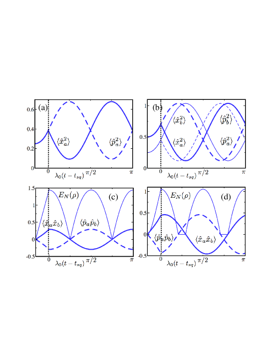
Figure 4: The covariances and the logarithmic negativity $E_{N}(\rho)$ for (a, c) $\Theta_{a}=\Theta_{b}=1$ and (b, d) $\Theta_{a}=2$ and $\Theta_{b}=1$. The dashed line at $t=t_{sq}$ signifies the end of the squeezing operation with $t_{sq}=0.5/\lambda_{0}$. Following squeezing, the beam splitter operation is applied for $\pi/\lambda_{0}$.

Starting at maximum entanglement at $t=t_{sq}$, we see $E_{N}(\rho)$ decreases to zero near $t=t_{sq}+\pi/4\lambda_{0}$ ($\varphi=\pi/4$) when the two resonator modes become separable, then returns to its maximum value at $t=t_{sq}+\pi/2\lambda_{0}$ ($\varphi=\pi/2$). At $t=t_{sq}+\pi/4\lambda_{0}$, we have

$$\widetilde{a}_{1}=\widetilde{b}_{2} = (\Theta_{a}+\Theta_{b})e^{-2\lambda_{0}t_{sq}}/8$$

$$\widetilde{a}_{2}=\widetilde{b}_{1} = (\Theta_{a}+\Theta_{b})e^{2\lambda_{0}t_{sq}}/8$$ (19)

showing a significant amount of squeezing for the quadrature fluctuations $\widetilde{a}_{1}=\langle\hat{x}_{a}^{2}\rangle$ and $\widetilde{b}_{2}=\langle\hat{p}_{b}^{2}\rangle$. The cross correlation at this point is $\widetilde{c}_{1}=\widetilde{c}_{2}=(\Theta_{a}-\Theta_{b})/8$. At finite temperature, as plotted in figure 4 (d), the negativity decreases to zero and the coupled resonators are in a separable state for a finite interval near $t=t_{sq}+\pi/4\lambda_{0}$ [26]. With increasing temperature, the duration of this interval increases as well, where the entanglement is diminished by thermal fluctuations. Meanwhile, the correlation between the logarithmic negativity and the covariance elements $c_{1,2}$ can also be seen in figure 4 (c) and (d).

In the special situation of zero temperature with $\Theta_{a}=\Theta_{b}$, as plotted in figure 4 (a) and (c), squeezed states can be generated for the resonator modes. Here we have $\widetilde{a}_{1}=\widetilde{b}_{2}$, $\widetilde{a}_{2}=\widetilde{b}_{1}$ and $\widetilde{c}_{1}=-\widetilde{c}_{2}$ at all times. When $t=t_{sq}+\pi/4\lambda_{0}$, the cross correlations as well as the entanglement vanish with $\widetilde{c}_{1,2}=E_{N}(\rho)=0$. When both modes are initially prepared in their ground states with $\Theta_{a,b}=1$, $\sqrt{\widetilde{a}_{1}\widetilde{a}_{2}}=1/4$. Thus, a squeezed state is generated in each resonator. For the coupled system of a nanomechanical resonator and an electrical resonator, this provides a novel way of generating squeezed states in the nanomechanical mode using linear parametric coupling.

5 Detection and the covariance matrix

A crucial requirement for studying the quantum properties of coupled resonators is the detection and verification of any engineered entanglement. Below we show that by only measuring the quadrature variances of one resonator – the electrical resonator – the full covariance matrix can be constructed.

In reality, measurement of the vibration of a nanomechanical mode is limited by the weak coupling between that mode and the detector. The electrical mode, in contrast, contains an electromagnetic signal that couples more strongly to the detector than the nanomechanical mode. Hence, the electrical mode provides an effective probe of the nanomechanical mode, which reduces the demand on the detector efficiency. For coupled electrical resonators, both modes can be measured simultaneously to directly test the theoretical results presented above.

The variances of the $\{\hat{x}_{a},\hat{x}_{b}\}$ quadratures at any time during the beam splitter operation are determined by three initial parameters: $a_{1},\,b_{1},\,c_{1}$, and similarly for the $\{\hat{p}_{a},\hat{p}_{b}\}$ quadratures. Measurements of the variances $\widetilde{b}_{1}$ (and $\widetilde{b}_{2}$), at three different times (in three sets of experiments with the beam splitter operation applied for different $\varphi$) that are linearly independent, can provide complete information about the entanglement dynamics of the coupled modes. For example, we choose to make measurements at $\varphi=0,\,\pi/4,\,\pi/2$ as defined above. At $\varphi=0$, $\widetilde{b}_{1}=b_{1}$ is measured; at $\varphi=\pi/2$, $\widetilde{b}_{1}=a_{1}$ is measured; at $\varphi=\pi/4$, $\widetilde{b}_{1}=\frac{a_{1}+b_{1}}{2}+c_{1}$ is measured, from which $c_{1}$ can be obtained by combining the previous results. Hence, the variances of the coupled modes can be uniquely determined by the measurements of the quadratures of (one of) the electrical modes. The times at which the measurements are performed can be adjusted. By choosing $\varphi=\pi/8,\,\pi/4,\,3\pi/8$, the quadrature fluctuations exceed thermal noise with $\widetilde{b}_{1}\gg\Theta_{b}/4$ in all three measurements as is shown in figure 4 (a, b). Note that to measure the squeezed state of a nanomechanical mode, a fast beam splitter operation with a phase $\pi/2$ can be applied before measuring the electrical mode. This operation transfers the states between the nanomechanical mode and the electrical mode, so that the subsequent measurements of the electrical resonator provide direct information of the nanomechanical mode.

This method provides a useful way of detecting the “hard” mechanical mode by detecting the “easy” electrical mode. Mechanical modes are in general “hard” to measure because they couple very weakly to detectors. By transferring the state of the mechanical mode to the electrical mode, which is in general “easy” to detect, we can clearly access the dynamical features of the mechanical mode. This state transfer technique was developed previously for phase qubits coupled to an electrical resonator [2]. Use of this method yields important information about entanglement by taking advantage of a dynamical process to reduce the requirements on the detector efficiency.

For the superconducting transmission line resonator, phase sensitive detection of the quadrature variables has been performed to reveal the vacuum Rabi splitting due to resonator-qubit coupling by measuring the transmission or reflection of a resonant signal [5] and for a resonator coupled to a nanomechanical beam to study the fluctuation of the quadrature variables approaching their quantum limit [RegalLehnert0801.1827, 9]. Alternatively, some work has studied the phase sensitive detection of resonator modes with a single electron transistor (SET) by mixing the signal of the resonator with a large radio-frequency reference signal and coupling the mixed signal to a SET detector [22, 29]. The nonlinear response of the SET enables a high resolution measurement of the electrical resonator [30]. The sensitivity of the measurement, however, can be limited by the detector noise. In the discussion above, only the detection of the covariance matrix of the coupled resonators was studied. Full characterization of the resonator states can be obtained by a quantum state tomography method as has been developed in the context of quantum optics [31].

6 Discussion and Conclusions

The effects studied in this paper can be tested with realistic parameters. Typical parameters for a nanomechancial resonator [7] are $\omega_{a}/2\pi=100\,\rm{MHz}$, $Q_{a}=10^{4}$, $d_{0}=50\,\rm{nm}$, and $\delta x_{0}=5\,\rm{fm}$. For a superconducting transmission line resonator [5], $\omega_{b}/2\pi=5\,\rm{GHz}$, $cL=4\,\rm{fF}$, and $Q_{b}=10^{4}$. With a bias voltage of $V_{x}^{0}=4\,\rm{V}$ and a coupling capacitance of $C_{x}^{0}=0.65\,\rm{fF}$, we find $\lambda_{0}/2\pi=6\,\rm{MHz}$ and the linear operations can be performed over a characteristic time scale of $t_{sq}=\pi/4\lambda_{0}\sim 130\,\rm{ns}$. For two coupled electrical resonators, choosing reasonable parameters for lumped-element quantum circuits [32] $\omega_{a}/2\pi=9\,\rm{GHz}$, $\omega_{b}/2\pi=10\,\rm{GHz}$, $L_{a}=L_{b}=5L_{c}=10M=500\,\rm{pH}$, $I_{o}=2.8\,\mu\rm{A}$, and a modulating flux drive like that described in section 2.2 gives $\lambda_{0}/2\pi=6\,\rm{MHz}$ so that the linear operations can also be performed for this system over a timescale of $t_{sq}\sim 130\,\rm{ns}$.

We didn’t discuss the effect of decoherence on the dynamics of the coupled resonator systems [33]. Many discussions can be found in the literature. The finite quality factors of both the electrical resonator and the nanomechanical resonator can limit the entanglement or squeezing in this scheme. Here, for a squeezing parameter $r_{2}=0.5$, we have $\bar{n}\sim 2\langle\hat{x}_{b}^{2}\rangle\sim 1$. Assuming a modest quality factor of $Q=10^{4}$ which is experimentally realizable, the decoherence time is on the order of $2\pi Q/(\bar{n}\omega_{b})\sim 2\,\mu\rm{s}\gg$ $t_{sq}$ sufficiently long enough to observe the entanglement and squeezing generated in these systems.

For the measurement process, we proposed a scheme using homodyne detection of the covariance matrix of the superconducting electrical resonator mode by applying the beam splitter operation at three different durations giving a full account of the covariance matrix of the coupled resonators. This avoids the difficulty of a direct measurement of the nanomechancial resonator mode. Considering a coupling capacitance of $C_{x}^{o}\sim 0.5\,\rm{fF}$ and a maximum possible bias voltage of $V_{x}\sim 10\,\rm{V}$, the demands on the detector efficiency are great if we consider directly measuring the quantum limited fluctuations of the nanomechanical resonator. For two coupled electrical resonators, direct detection on both resonators together can reveal the covariances for all controlled operations, extremely useful for testing these types of systems and the schemes we have described for generating entanglement and squeezed states.

In conclusion, we studied the generation of controllable entanglement and squeezing in coupled macroscopic resonators, in particular, a nanomechanical-electrical resonator, by applying parametrically modulated linear coupling. Two systems are studied in detail: the coupling between a nanomechanical resonator and a superconducting transmission line resonator, and the coupling between two superconducting electrical resonators. The parametric coupling is calculated in both cases. Furthermore, effective detection of the entanglement and squeezing in one of the modes can be achieved by measuring the other (electrical) mode. We have considered specific, reasonable operating parameters and find that both of these systems should be experimentally feasible. Squeezing of the nanomechanical system, although difficult, should be possible at very low temperatures whereas the relatively simple two coupled electrical resonator system should show clear squeezing for a variety of typical operating conditions. The scheme studied here is a key component for entanglement based quantum information protocols such as quantum teleportation in a solid-state network [23].

References

References

- [1] Majer J, Chow J M, Gambetta J M, Koch J, Johnson B R, Schreier J A, Frunzio L, Schuster D I, Houck A A, Wallraff A, Blais A, Devoret M H, Girvin S M, Schoelkopf R J 2007 Nature 449 443
- [2] Sillanpä M A, Park J I, Simmonds R W 2007 Nature 449 438
- [3] Hofheinz M, Weig E M, Ansmann M, Bialczak R C, Lucero E, Neeley M, O Connell A D, Wang H, Martinis J M, Cleland A N 2008 Nature 454 310
- [4] Johansson J, Saito S, Meno T, Nakano H, Ueda M, Semba K, Takayanagi H 2006 Phys. Rev. Lett. 96 127006
- [5] Wallraff A, Schuster D I, Blais A, Frunzio L, Huang R S, Majer J, Kumar S, Girvin S M, and Schoelkopf R J 2004 Nature 431 162 Blais A, Huang R S, Wallraff A, Girvin S M, and Schoelkopf R J 2004 Phys. Rev. A 69 062320 Chiorescu I, Bertet P, Semba K, Nakamura Y, Harmans C J P M, and Mooij J E 2004 Nature 431 159 Koch R H, Keefe G A, Milliken F P, Rozen J R, Tsuei C C, Kirtley J R , and DiVincenzo D P 2006 Phys. Rev. Lett. 96 127001
- [6] Makhlin Y Schön G and Shnirman A 2001 Rev. Mod. Phys. 73 357
- [7] Knobel R G and Cleland A N 2003 Nature 424 291 LaHaye M D, Buu O, Camarota B, Schwab K C 2004 Science 304 74
- [8] Blencowe M P 2004 Phys. Rep. 395 159
- [9] Regal C A, Teufel J D, Lehnert K W 2008 Nature Phys. 4, 555 Teufel J D, Harlow J W, Regal C A, Lehnert K W 2008 preprint arXiv:0807.3585
- [10] Braunstein S L and van Loock P 2005 Rev. Mod. Phys. 77 513
- [11] Tian L 2005 Phys. Rev. B 72 195411
- [12] Jacobs K 2007 Phys. Rev. Lett. 99 117203
- [13] Yuan H and Lloyd S 2007 Phys. Rev. A 75 052331
- [14] Niskanen O, Harrabi K, Yoshihara F, Nakamura Y, Lloyd S, Tsai J S 2007 Science 316 723
- [15] Movshovich R, Yurke B, Kaminsky P G, Smith A D, Silver A H, Simon R W, Schneider M V 1990 Phys. Rev. Lett. 65 1419
- [16] Rabl P, Shnirman A, and Zoller P 2004 Phys. Rev. B 70 205304
- [17] Ruskov R, Schwab K, and Korotkov A N 2005 Phys. Rev. B 71 235407
- [18] Moon K and Girvin S M 2005 Phys. Rev. Lett. 95 140504
- [19] Zhou X X and Mizel A 2006 Phys. Rev. Lett. 97 267201
- [20] Eisert J, Plenio M B, Bose S, and Hartley J 2004 Phys. Rev. Lett. 93 190402 Pirandola S, Vitali D, Tombesi P, and Lloyd S 2006 Phys. Rev. Lett. 97 150403
- [21] Naik A, Buu O, LaHaye M D, Armour A D, Clerk A A, Blencowe M P, Schwab K C 2006 Nature 443 193 and references there in.
- [22] Sarovar M, Goan H S, Spiller T P, and Milburn G J 2005 Phys. Rev. A 72 062327
- [23] Tian L and Carr S 2006 Phys. Rev. B 74 125314
- [24] van den Brink A M, Berkley A J, and Yalowsky M 2005 New J. Phys. 7 230
- [25] Ferraro A, Olivares S, Paris M G A Gaussian states in continuousvariable quantum information 2005 arXiv:quant-ph/0503237
- [26] Simon R 2000 Phys. Rev. Lett. 84 2726 Duan L M, Giedke G, Cirac J I, and Zoller P 2000 Phys. Rev. Lett. 84 2722
- [27] Vidal G and Werner R F 2002 Phys. Rev. A 65 032314 Wolf M M, Giedke G, Krüger O, Werner R F, and Cirac J I 2004 Phys. Rev. A 69 052320
- [28] Altomare F, Park J I, Simmonds R W 2008 Preparation of cavity fock states -unpublished
- [29] Knobel R, Yung C S, and Cleland A N 2002 Appl. Phys. Lett. 81 532 Swenson L J, Schmidt D R, Aldridge J S, Wood D K, and Cleland A N 2005 Appl. Phys. Lett. 86 173112
- [30] Schoelkopf R J, Wahlgren P, Kozhevnikov A A, Delsing P, and Prober D E 1998 Science 280 1238 Tien P K and Gordon J P 1963 Phys. Rev. 129 647 Turek B A, Lehnert K W, Clerk A, Gunnarsson D, Bladh K, Delsing P, Schoelkopf R J 2005 Phys. Rev. B 71, 193304 Blencowe M P and Wybourne M N 2000 Appl. Phys. Lett. 77 3845 Mozyrsky D, Martin I, and Hastings M B 2004 Phys. Rev. Lett. 92 018303 Clerk A A and Girvin S S 2004 Phys. Rev. B 70 121303(R)
- [31] Leibfried D, Blatt R, Monroe C, and Wineland D 2003 Rev. Mod. Phys. 75 281
- [32] McDermott R, Simmonds R W, Steffen M, Cooper K B, Cicak K, Osborn K D, Oh S, Pappas D P, Martinis J M 2005 Science 307 1299 Oliver W D, Yu Y, Lee J C, Berggren K K, Levitov L S, Orlando T P 2005 Science 310 1653 Bertet P, Chiorescu I, Burkard G, Semba K, Harmans C J P M, DiVincenzo D P, Mooij J E 2005 Phys. Rev. Lett. 95 257002
- [33] Schützhold R and Tiersch M 2005 J. Opt. B: Quantum Semiclass. Opt. 7 S120 Caldeira A O and Leggett A J 1983 Physica A 121 587