The parametric oscillation threshold of semiconductor microcavities in the strong coupling regime

Abstract

The threshold of triply resonant optical parametric oscillation in a semiconductor microcavity in the strong coupling regime is investigated. Because of the third-order nature of the excitonic nonlinearity, a variety of different behaviours is observed thanks to the interplay of parametric oscillation and optical bistability effects. The behaviour of the signal amplitude and of the quantum fluctuations in approaching the threshold has been characterized as a function of the pump, signal and idler frequencies.

I Introduction

Triply resonant optical parametric oscillation (OPO) OPO_general ; OPO_special has been recently observed stevenson ; houdre ; baumberg in semiconductor microcavities in the strong coupling regime microcavity_review1 ; microcavity_review2 , and has attracted a good deal of attention from the point of view of both fundamental physics and possible technological applications. The peculiar dispersion relation of polaritons in the strong coupling regime allows to simultaneously satisfy the resonance condition for the pump, signal and the idler modes. Together with the enormous value of the excitonic nonlinearities, the possibility of easy phase matching results in a low threshold intensity, making these systems very promising candidates for low-power OPO applications.

A complete theoretical description of the OPO dynamics of such systems is not only very important in view of the optimisation of the device operation, but also deserves a certain interest from the point of view of nonlinear dynamics as many interesting phenomena can occur due to the interplay of optical bistability and parametric oscillation iac-superfl ; whittaker05 , and to the nontrivial spatial field dynamics in the transverse plane whittaker_last ; pattern .

As shown by several theoretical papers that have appeared on the subject, a rather complex phenomenology is found already at the level of the three-mode approximation, where the classical nonlinear optical wave equation is projected onto the three pump, signal and idler modes whittaker05 ; whittaker01 ; ciuti-rev ; gippius . Available experimental data appear to confirm this point: in particular, both continuous baumberg ; dasbach and discontinuous baas behaviours have been experimentally shown for the signal intensity in the neighborhood of the threshold point. Although some analogies have been drawn with what is known about $\chi^{(2)}$ OPO dynamics in standard passive media OPO_general ; OPO_special ; TROPO ; chi2OPO ; lugiato , no complete investigation has appeared yet for the case of semiconductor microcavities in the strong coupling regime, neither from the experimental nor from the theoretical points of view.

The optical nonlinearity of the microcavity system under investigation originates from collisional exciton-exciton interactions and is therefore of the $\chi^{(3)}$ type. This means that it not only provides the parametric interaction necessary for the parametric oscillation, but is also responsible for significant mean-field frequency shifts of the modes. This makes the nonlinear dynamics of the mode amplitudes much richer than in $\chi^{(2)}$ OPOs lugiato . Pioneering theoretical work in this direction has recently appeared in Ref. whittaker05, .

The purpose of the present paper is to provide a systematic and quantitative study of the OPO threshold in semiconductor microcavities in the strong coupling regime. Depending on the pump laser frequency, and the signal, pump and idler mode frequencies, several regimes are to be distinguished, where the system behaviour is radically different.

The paper is organized as follows: our model of the microcavity is introduced in Sec.II. Optical limiting and optical bistability in the pump only solution are discussed in Sec.III.1. General concepts about the stability of the solution with respect to pump-only and to parametric instabilities are given in Sec.III.2. The following Secs.III.3-III.7 are devoted to characterize the parametric threshold as a function of the incident pump angle, the internal and the incident intensities and to find the optimal choice to minimize the threshold intensity. Quantitative estimations are provided in Sec.III.8, where a comparison is made with other realizations of OPOs based on passive $\chi^{(2)}$ and $\chi^{(3)}$ materials. The kind of bifurcation at the onset of the OPO emission is investigated in Sec.IV. Depending on whether the pump-only solution is in the optical limiter or in the optical bistability regimes, parametric emission is shown to set in either in a continuous or in a discontinuous way. The close relationship between the nature of the instability point and the behaviour of the quantum fluctuations as the threshold is approached is pointed out in Sec.IV.4. Conclusions are finally drawn in Sec.V.

II Polariton model

A sketch of the physical system under investigation is shown in Fig.1: a planar DBR (Distributed Bragg Reflector) semiconductor microcavity containing a few quantum wells strongly coupled to the cavity mode. The elementary excitations of this system consist of exciton-polaritons, i.e. coherent superpositions of cavity photons and excitons. Polaritons combine the very strong $\chi^{(3)}$ optical nonlinearity originating from exciton-exciton collisional interactions to the peculiar dispersion relation as a function of the in-plane wavevector ${\mathbf{k}}$ that is shown in Fig.1: these facts make them extremely well suited for triply-resonant optical parametric oscillator applications, as it has indeed been experimentally demonstrated in recent years stevenson ; houdre ; baumberg .

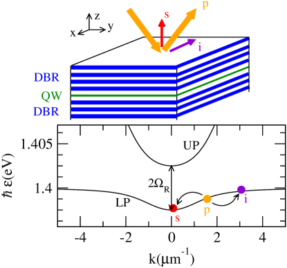
Figure 1: Upper panel: sketch of the microcavity system and of the parametric process under consideration. Lower panel: lower polariton (LP) and upper polariton (UP) dispersion at linear regime. The cavity photon dispersion is $\omega_{C}(k)=\omega_{C}^{0}\,\sqrt{1+{k^{2}}/{k_{z}^{2}}}$ with $\hbar\omega^{0}_{C}=1.4$ eV and $k_{z}=20\,\mu\rm m^{-1}$. The exciton dispersion is flat and resonant with the $k=0$ cavity mode $\omega_{X}=\omega_{C}^{0}$. The exciton-photon Rabi coupling is $\hbar\Omega_{R}=2.5$ meV. The dots indicate the signal, pump and idler modes, the arrows show the triply resonant parametric process under investigation.

A mean-field description of the cavity-polariton field dynamics can be developed in terms of a nonlinear wave equation with a third-order nonlinearity ciuti-rev ; iac-superfl . Under the assumption that the dynamics takes place in the lower polariton branch and the population of the upper polariton branch remains negligible, the theoretical description can be simplified by restricting it to the lower polariton only. For the sake of simplicity, we shall focus our attention on the case of a circularly polarized pump beam. As the circular polarization of the polariton field is preserved by the nonlinear interactions and the longitudinal-transverse splitting kavokinpss ; langbein is much smaller than both the linewidth $\gamma$ and the nonlinear interaction energy, the circular polarization is almost completely transferred to the signal and idler beams.

Under these assumptions, the polariton dynamics can be written in terms of a nonlinear wave equation for a single-component $k$-space polariton field $\psi_{LP}({\mathbf{k}})$:

$$i\frac{d}{dt}\psi_{LP}({\mathbf{k}})=\left[\epsilon(k)-i\frac{\gamma({\mathbf{k}})}{2}\right]\psi_{LP}({\mathbf{k}})+F_{p}({\mathbf{k}})\,\,e^{-i\omega_{p}t}\\ +\sum_{{\mathbf{q}}_{1},{\mathbf{q}}_{2}}g_{{\mathbf{k}},{\mathbf{q}}_{1},{\mathbf{q}}_{2}}\,\psi^{*}_{LP}({\mathbf{q}}_{1}+{\mathbf{q}}_{2}-{\mathbf{k}})\,\psi_{LP}({\mathbf{q}}_{1})\,\psi_{LP}({\mathbf{q}}_{2}).$$ (1)

The field $\psi_{LP}({\mathbf{k}})$ is here normalized in such a way that its square modulus $|\psi_{LP}({\mathbf{k}})|^{2}$ equals the number of polaritons with momentum ${\mathbf{k}}$ per unit area. $\epsilon({\mathbf{k}})$ is the dispersion relation of the lower polariton and $\gamma({\mathbf{k}})$ is the momentum-dependent loss rate. Throughout the present paper, the exciting laser field is taken as a monochromatic and continuous wave coherent field at $\omega_{p}$ with a plane-wave spatial profile at ${\mathbf{k}}_{p}$ and a circular polarization. The driving amplitude $F_{p}({\mathbf{k}})$ can be related to the incident power density $I_{inc}$ by using the input-output formalism gardiner ; input-output ; baas :

$$F_{p}({\mathbf{k}})=\delta_{{\mathbf{k}},{\mathbf{k}}_{p}}C({\mathbf{k}}_{p})\sqrt{\frac{\gamma_{rad}I_{inc}}{N_{tr}\hbar\omega_{p}}}.$$ (2)

$\gamma_{rad}$ is here the radiative decay rate of the cavity-photon due to the finite mirror transmittivity; the parameter $N_{tr}$ specifies whether the cavity is a single-sided cavity with a perfectly reflecting back mirror ($N_{tr}=1$), or a symmetric cavity with equal transmission through both the front and back mirrors ($N_{tr}=2$).

The third-order nonlinear interaction term takes into account exciton-exciton collisional interactions. As the wavevectors involved in the present discussion are much smaller than the inverse excitonic radius, the exciton-exciton coupling constant in a single quantum well can be approximated by a momentum-independent ${\bar{g}}$. If $N_{QW}$ quantum wells are present in the cavity, identically coupled to the cavity mode, the bright excitonic excitation is delocalized over all of them and the effective excitonic coupling constant is $g={\bar{g}}/N_{QW}$. In the polaritonic basis, a non-trivial momentum dependence appears via the Hopfield coefficients $X({\mathbf{k}})$ and $C({\mathbf{k}})$ quantifying the excitonic and cavity-photonic components of the lower polariton:

$$g_{{\mathbf{k}},{\mathbf{q}}_{1},{\mathbf{q}}_{2}}=g\,X^{*}({\mathbf{k}})\,X^{*}({\mathbf{q}}_{1}+{\mathbf{q}}_{2}-{\mathbf{k}})\,X({\mathbf{q}}_{1})\,X({\mathbf{q}}_{2}).$$ (3)

Although no conclusive experimental nor theoretical analysis has been reported yet, the theoretical prediction $\hbar{\bar{g}}\approx 1.5\times 10^{-5}\,\textrm{eV}\,\mu\textrm{m}^{2}$ based on the Born approximation Born_approx appears to be in reasonable agreement with available experimental data microcavity_review1 ; microcavity_review2 .

In order to focus our discussion of the basic OPO dynamics, we shall not consider here the effect of the disorder: in recent high quality III-V samples the effect of the disorder can in fact be weak enough for it to be neglected on the scale of the polaritonic linewidth. In this case, it is legitimate to approximate the mode eigenfunctions as plane waves. On the other hand, the disorder is much stronger in II-VI samples, where it has been shown to have dramatic consequences on polariton BEC Pol-BEC . These effects are highly non-trivial already at equilibrium fisher and are expected to become even more complex because of the interplay with the nonlinear dynamics: the complete analysis of them goes far beyond the scope of the present paper and is left to future work.

To conclude the section, it is interesting to note that the applicability range of the wave equation (1) is not limited to semiconductor planar OPOs, but can be extended to describe other setups, e.g. planar cavities containing a slab of passive $\chi^{(3)}$ material. In this case, no excitonic resonance exists, and the polariton reduces to a bare cavity-photon. As both the coupling to external radiation and the optical nonlinearity act on the same photonic degree of freedom, one has simply to set $X=C=1$ and calculate the nonlinear coupling constant using the nonlinear susceptibility of the medium under consideration:

$$\hbar g={\mathcal{C}}\,\chi^{(3)}\,\frac{(\hbar\omega_{p})^{2}}{\epsilon_{\rm lin}^{2}d}.$$ (4)

The numerical factor ${\mathcal{C}}$ of order one takes into account the details of the geometry under investigation. Typical values of $\chi^{(3)}$ of materials specifically designed for nonlinear optical applications range up to something of the order of $10^{-9}\,\textrm{esu}$ NLO_mat . For a $\lambda/2$ cavity, these values correspond to a nonlinear coupling constant of the order of $\hbar g\approx 5\times 10^{-9}\,\textrm{eV}\,\mu\textrm{m}^{2}$, orders of magnitude lower than the value $\hbar{\bar{g}}\approx 1.5\times 10^{-5}\,\textrm{eV}\,\mu\textrm{m}^{2}$ previously mentioned for semiconductor microcavities in the strong coupling regime. This explains the present interest of semiconductor microcavities for low-power nonlinear optical applications, as well as for fundamental studies of the interplay of nonlinear dynamics and quantum fluctuations coh_length ; verger .

III The parametric threshold

III.1 The pump only solution

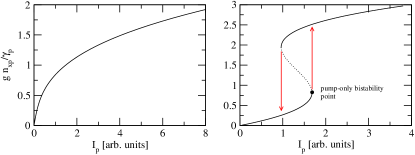
Figure 2: Polariton density in the pump mode as a function of the driving intensity $I_{p}=|F_{p}|^{2}$ for a pump wave vector of $k_{p}=1.19\mu\textrm{m}^{-1}$, which corresponds to $\epsilon_{p}=1.39845\,\textrm{eV}$. The left graph is in the optical limiter regime ($\omega_{p}=\epsilon_{p}$), whereas the right one is in the bistability regime ($\omega_{p}=\epsilon_{p}+1.5\gamma_{p}$). The red arrows show the jump in polariton density for an upward (right arrow) and downward (left arrow) ramp of the laser intensity. The dotted part of the curve is dynamically unstable. Same cavity parameters as in Fig.1.

Among the different ${\mathbf{k}}$ modes, only the one at ${\mathbf{k}}={\mathbf{k}}_{p}$ contains a source term in its equation of motion (1). An exact solution of the full set of equations of motion (1) can therefore be found in the form

$$\psi_{LP}(x,t)=P\,e^{i({\mathbf{k}}_{p}{\mathbf{x}}-\omega_{p}t)},$$ (5)

with the amplitude $P$ fixed by the condition:

$$[\epsilon_{p}-\omega_{p}-\frac{i}{2}\gamma_{p}+g|X(k_{p})|^{4}|P|^{2}]P+F_{p}=0.$$ (6)

Here $\epsilon_{p}=\epsilon({\mathbf{k}}_{p})$ is the frequency of the pump mode at linear regime and $\gamma_{p}=\gamma({\mathbf{k}}_{p})$ the corresponding linewidth; the effect of the third-order nonlinearity is to renormalize the pump mode frequency by a mean-field shift proportional to the mode excitonic population $n_{xp}=|X({\mathbf{k}}_{p})|^{2}|P|^{2}$. This effect, absent in $\chi^{(2)}$ cavities, is responsible for the the qualitatively different behaviours bistability that can be observed depending on the sign of the detuning of the pump frequency $\omega_{p}$ with respect to the polariton energy $\epsilon(k_{p})$.

Fig.2 shows the excitonic density in the pump mode $n_{xp}$ as a function of the driving intensity $I_{p}=|F_{p}|^{2}$ which is proportional (but not identical) to the incident laser intensity $I_{inc}$ [See Eq.(2)]. When the pump frequency is below or close to resonance $\omega_{p}-\epsilon({\mathbf{k}}_{p})<\sqrt{3}\,\gamma({\mathbf{k}}_{p})/2$, we are in the so-called optical limiter regime, in which the population $n_{xp}$ of the ${\mathbf{k}}_{p}$ mode monotonically increases as a function of the driving intensity $I_{p}$ (left panel).

For blue-detuned pump frequencies $\omega_{p}-\epsilon({\mathbf{k}}_{p})>\sqrt{3}\,\gamma({\mathbf{k}}_{p})/2$, a positive feedback of the nonlinearity occurs and hysteretic behaviour can be instead observed, as shown in the right panel of Fig.2 and experimentally demonstrated in Ref. baas-bist, . For increasing laser intensity, the pump mode population follows the lower branch until its endpoint is reached, and then it jumps to the upper branch as indicated by the arrow. If the driving intensity is later ramped down, the system keeps following the upper branch until its endpoint, and only here the pump mode population jumps back to the lower branch. Hysteretic behaviour is apparent, as the upward and downward jump points do not coincide.

III.2 Dynamical stability of the pump-only state

As usual in nonlinear dynamical systems, finding a solution is not sufficient, as one has to verify its dynamical stability. Optical parametric oscillation, as well as the instability of the central branch of the hysteresis loop are in fact due to the solution (6) becoming dynamically unstable.

As the planar cavity supports a continuum of independent modes with different in-plane wavevectors, dynamical stability of the pump only solution (6) has to be checked with respect to perturbations with any wave vector ${\mathbf{k}}_{s}$:

$$\psi_{LP}({\mathbf{x}},t)=Pe^{-i\omega_{p}t+i{\mathbf{k}}_{p}{\mathbf{x}}}+u({\mathbf{k}}_{s})e^{-i[\omega_{p}+\omega({\mathbf{k}}_{s})]t+i{\mathbf{k}}_{s}x}\\ +v^{*}({\mathbf{k}}_{s})e^{-i[\omega_{p}-\omega^{*}({\mathbf{k}}_{s})]t+i(2{\mathbf{k}}_{p}-{\mathbf{k}}_{s}){\mathbf{x}}}.$$ (7)

Substituting this expression in Eq.(1) and keeping only linear terms in the fluctuations $u$ and $v$, one gets to the following eigenvalue problem ciuti-lum

$$L({\mathbf{k}}_{s})\,w({\mathbf{k}}_{s})=\omega({\mathbf{k}}_{s})\,w({\mathbf{k}}_{s})$$ (8)

where the two-component vector $w({\mathbf{k}}_{s})=[u({\mathbf{k}}_{s}),v({\mathbf{k}}_{s})]^{T}$ and the 2x2 matrix $L({\mathbf{k}}_{s})$ is

$$L({\mathbf{k}}_{s})=\left(\begin{array}[]{cc}\epsilon_{s}-\omega_{p}+2g|X_{s}|^{2}|X_{p}|^{2}|P|^{2}-i\frac{\gamma_{s}}{2}&gX^{*}_{s}X_{i}X_{p}^{2}P^{2}\\ -gX_{s}X^{*}_{i}X_{p}^{*2}P^{*2}&-\epsilon_{i}+\omega_{p}-2g|X_{i}|^{2}|X_{p}|^{2}|P|^{2}-i\frac{\gamma_{i}}{2}\end{array}\right).$$ (9)

The matrix $L({\mathbf{k}}_{s})$ couples the fluctuations in the ${\mathbf{k}}_{s}$ and ${\mathbf{k}}_{i}=2{\mathbf{k}}_{p}-{\mathbf{k}}_{s}$ modes, called in the following the signal and the idler modes. Short-hand notations have been here introduced to simplify the expressions: $X_{s,i}=X({\mathbf{k}}_{s,i})$ are the excitonic Hopfield coefficients of the signal/idler modes, $\epsilon_{s,i}=\epsilon({\mathbf{k}}_{s,i})$ are the signal and idler mode frequencies and $\gamma_{s,i}=\gamma({\mathbf{k}}_{s,i})$ are the corresponding loss rates. Dynamical stability is ensured if the imaginary parts of all eigenvalues of $L({\mathbf{k}}_{s})$ are negative ${\rm Im}[\omega_{\pm}({\mathbf{k}}_{s})]<0$ for all wavevectors ${\mathbf{k}}_{s}$. These can be written as:

$${\rm Im}\{\omega_{\pm}({\mathbf{k}}_{s})\}=-\frac{\gamma_{s}+\gamma_{i}}{4}\pm{\rm Im}\left\{\sqrt{[(\epsilon_{si}-\omega_{p})+g(|X_{s}|^{2}+|X_{i}|^{2})n_{xp}-i\frac{\gamma_{s}-\gamma_{i}}{4}]^{2}-g^{2}\,|X_{s}|^{2}|X_{i}|^{2}n_{xp}^{2}}\right\},$$ (10)

Note that the pump mode frequency $\epsilon_{p}$ does not directly appear in the expression (10) of the eigenvalues, but it is only indirectly involved via the pump-only solution (6), which fixes $n_{xp}$. The frequencies of the signal and idler modes are involved in (10) only via their average value $\epsilon_{si}=[\epsilon_{s}+\epsilon_{i}]/2$.

Two kinds of physically distinct instabilities can arise. A single-mode instability arises when the equation of motion for the pump mode alone – neglecting all interactions with other modes – is dynamically unstable. This instability is found when $L({\mathbf{k}}_{s})$ has an eigenvalue with a positive imaginary part for ${\mathbf{k}}_{s}={\mathbf{k}}_{p}$. As in this case ${\mathbf{k}}_{i}={\mathbf{k}}_{s}={\mathbf{k}}_{p}$, this instability involves the ${\mathbf{k}}_{p}$ mode only, and for this reason it is called single-mode. It is easy to verify iac-superfl that the pump-only solution (6) is single-mode unstable in the central branch of the bistability curve (marked with a dotted line in Fig.2b). At the turning points of the bistability curve a stable and an unstable solution meet, so that the bifurcation is of the saddle node type hale .

Our interest is however more focussed on instabilities of the second kind, i.e. for ${\mathbf{k}}_{s}\neq{\mathbf{k}}_{p}$: this parametric instability signals the onset of parametric oscillation with a finite intensity appearing in a pair of distinct signal/idler modes at ${\mathbf{k}}_{s,i}$. From the point of view of bifurcation theory, the parametric instability profoundly differs from the single-mode one. As we shall see in the following, the pump-only solution still exists beyond the threshold point, but it is no longer stable for an eigenvalue of the linear stability matrix $L({\mathbf{k}})$ has crossed the real axis: the bifurcation is then of the Hopf type hale and is accompanied by a spontaneous breaking of a signal/idler $U(1)$ phase rotation symmetry Goldstone .

III.3 Available range of signal/idler frequencies

In the present paper, we shall not address the problem of the determination of the wavevectors ${\mathbf{k}}_{s,i}$ which are actually selected by the parametric process above threshold. This is a very complicate problem and is postponed to a forthcoming publication pattern . Here we shall limit ourself to a study of the lower threshold for parametric emission: the parametric oscillation dynamics will be initiated as soon as the incident intensity exceeds the threshold value for some pair of signal/idler modes.

For each value of pump wavevector ${\mathbf{k}}_{p}$, it is important to characterize the range of $\epsilon_{si}$ that can be obtained when the signal/idler wavevectors ${\mathbf{k}}_{s,i}$ are spanned through all different polariton states: the search for the minimum value of the threshold has in fact to be restricted to the region of $\epsilon_{si}$ values which are actually available.

This point is addressed in Fig.3. In the left panel, the behaviour of the detuning $(\epsilon_{si}-\epsilon_{p})$ as a function of $k_{s}$ is shown for three different values of $k_{p}$ and the yellow region in the right panel summarizes the accessible detunings as a function of $k_{p}$. For small $k_{p}$, the $\epsilon_{si}$ vs. $k_{s}$ curve has a single minimum at $k_{s}=k_{p}$ where $\epsilon_{si}=\epsilon_{p}$, and then tends to a finite limit for large $k_{s}$ ($\epsilon(k)$ has a finite limit for large $k$). For larger values of $k_{p}$, negative values $\epsilon_{si}-\epsilon_{p}<0$ can be reached. The minimum is in fact split in two separate minima whittaker05 , symmetrically located around the pump angle as required by the symmetry of $\epsilon_{si}$ under exchange of the signal and idler modes. The upper limit of the available band monotonically decreases as a function of $k_{p}$, due to the corresponding increase of $\epsilon_{p}$. In particular, it tends to $0$ for large values of $k_{p}$.

Figure 3: Left panel: plot of $\epsilon_{si}$ as a function of $k_{s}$ for fixed values of $k_{p}=0$ (full black), $k_{p}=1.19\,\mu{\textrm{m}}^{-1}$ (dashed red), $k_{p}=1.4\,\mu\textrm{m}^{-1}$ (dotted blue). The vertical lines show the value of the pump wave vector. Right panel: band of available $\epsilon_{si}$ values as a function of $k_{p}$. The horizontal green line shows the optimal detuning $\Delta_{si,p}^{opt}$ (see Sec.III.6 below), the vertical lines indicate the $k_{p}$ values corresponding to the curves in the left panel. Cavity parameters as in Fig.1, equal damping rates $\gamma_{s,p,i}=\gamma$ with $\hbar\gamma=0.25$ meV.

III.4 Pump intensity $n_{xp}$ at the parametric threshold

As it often happens in nonlinear optical systems, it is useful to study the parametric threshold first in terms of the internal light intensity in the cavity, in our case the excitonic pump mode population $n_{xp}$. Connection to the incident intensity $I_{inc}$ will be then made in the next subsection. As we are still left with several parameters, namely $\gamma_{i}/\gamma_{s}$, $X_{s}^{2}$ and $X_{i}^{2}$, we are forced to restrict the discussion to some illustrative examples. The qualitative features are however quite robust with respect to their variations. Let us begin from the $\gamma_{s}=\gamma_{i}=\gamma_{si}$ case: as the argument of the square root in eq.(10) is purely real, the calculations are in this case the simplest.

The pump mode population $n_{xp}$ at the parametric threshold is plotted in Fig.4 as a function of $\omega_{p}-\epsilon_{si}$ for two possible choices of the Hopfield coefficients. No qualitative differences are visible, but only quantitative ones. The main feature of these curves is the fact that parametric oscillation can only take place for sufficiently large values of $\omega_{p}-\epsilon_{si}$. The hatched regions indeed indicate where parametric oscillation can never take place, no matter how large the population of the pump mode is. Remarkably, the minimum value of the threshold population is reached just before the endpoint of the curves.

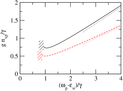
Figure 4: Threshold excitonic density in the pump mode as a function of the pump laser detuning from the average signal/idler natural frequencies. The full black curve refers to a semiconductor microcavity for which the Hopfield coefficients are $X_{s}=X(0)$ and $X_{i}=X(2k_{\rm magic})$. The dashed red curve refers to the case of a cavity containing a passive nonlinear material for which $X_{j}=1$. The curves do not continue through the hatched region at the left hand side where parametric oscillation can never take place. The dotted lines represent the approximation (14). Cavity parameters as in Fig.3.

Simple physical arguments can be put forward to explain these features. In a $\chi^{(3)}$ parametric oscillator, the nonlinearity not only provides the parametric coupling between the signal and idler modes via the off-diagonal terms in the matrix (9), but is at the same time responsible for a mean-field blue shift of the signal and idler mode frequencies by $2\,g\,|X_{s,i}|^{2}\,n_{xp}$. Once this shift is taken into account, the resonance condition for the parametric process is renormalized to

$$\omega_{p}=\epsilon_{si}+g(|X_{s}|^{2}+|X_{i}|^{2})n_{xp}.$$ (11)

From (10), it is easy to see that the minimum value of the threshold

$$n_{xp}^{min}=\frac{\gamma_{si}}{2g|X_{s}|\,|X_{i}|}$$ (12)

is indeed attained when this condition is satisfied. Combining (11) and (12) gives the optimal detuning

$$\omega_{p}-\epsilon_{si}=\gamma_{si}\,\frac{|X_{s}|^{2}+|X_{i}|^{2}}{2|X_{s}\,X_{i}|},$$ (13)

which corresponds to the position of the minimum of the curves plotted in Fig.4.

On the other hand, for large and positive values of the detuning $\omega_{p}-\epsilon_{si}\gg\gamma_{si}$, the threshold grows in a linear way as a function of $\omega_{p}-\epsilon_{si}$

$$n_{xp}=\frac{\omega_{p}-\epsilon_{si}}{g(|X_{s}|^{2}+|X_{i}|^{2}+|X_{s}X_{i}|)}.$$ (14)

Finally, for $\omega_{p}-\epsilon_{si}<0$ the well-known inequality $(|X_{s}|^{2}+|X_{i}|^{2})^{2}>|X_{s}|^{2}\,|X_{i}|^{2}$ implies that (10) can never be zero for any value of $n_{xp}$, so that parametric oscillation can never take place in this case. The mean field shifts push in fact the signal/idler modes out of resonance before the parametric coupling can overcome the damping rate $\gamma_{si}$.

III.5 Laser intensity at threshold

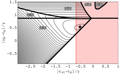
Figure 5: Contour plot of the threshold laser intensity as a function of the detunings. The decay rates for the pump, signal and idler modes are taken equal to $\gamma_{s,p,i}=\gamma$ and the Hopfield coefficients $X_{s}=X(0)$, $X_{p}=X(k_{\rm magic})$ and $X_{i}=X(2k_{\rm magic})$. The lowest contour line in the plot is at $1.05I_{inc}^{min}$, where the minimum of the threshold intensity $I_{inc}^{min}$ is attained at the point indicated by a star $\star$ and is defined in Eq.(18) below. The difference between the contours is $0.3I_{inc}^{min}$. The letters (A)-(E) indicate the regions of qualitatively different behaviours; the corresponding pump-only characteristic curves are shown in Fig.6. The red-shaded area indicates the values of $\epsilon_{si}-\epsilon_{p}$ that are available for the value of the pump angle $k_{p}=1.4\mu\rm m^{-1}$, corresponding to the red curve in Fig.3.

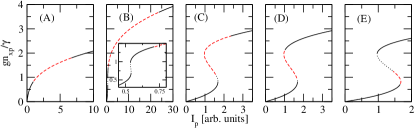
Figure 6: Pump-only characteristic curves for different values of the detunings. Instabilities with respect to a parametric oscillation process at a given $\epsilon_{si}$ are indicated as red dashed, pump-only instabilities are indicated as black dotted. Arbitrary units for $I_{p}$ are the same in all panels. The labels of the plots correspond to the different regions in Fig.5: (A) parametric oscillation in the optical limiter regime ($\epsilon_{si}-\epsilon_{p}=-1.5\gamma,\;\omega_{p}-\epsilon_{p}=0$); ; (B) bistability regime: parametric oscillation threshold above the pump-only bistability region ($\epsilon_{si}-\epsilon_{p}=-2\gamma,\;\omega_{p}-\epsilon_{p}=0.9\gamma$), the inset shows the bistability region more in detail; (C) bistability regime: parametric oscillation threshold at pump-only bistability region ($\epsilon_{si}-\epsilon_{p}=-0.6\gamma,\;\omega_{p}-\epsilon_{p}=1.5\gamma$); (D) bistability regime: parametric oscillation threshold not reachable with upward ramp in laser intensity ($\epsilon_{si}-\epsilon_{p}=-0.2\gamma,\;\omega_{p}-\epsilon_{p}=1.5\gamma$); (E) bistability regime: parametric oscillation threshold before pump-only instability point ($\epsilon_{si}-\epsilon_{p}=0.4\gamma,\;\omega_{p}-\epsilon_{p}=1.5\gamma$).

In the previous section we have determined the value of the pump mode population $n_{xp}$ at the threshold for parametric oscillation. The value of the corresponding laser intensity is then obtained by using (6). Care has to be paid to the fact that single-mode instabilities may make some branches of the bistability loop dynamically unstable and therefore not reachable in an actual experiment. Again, this feature is typical whittaker05 of a $\chi^{(3)}$ OPO and is absent in $\chi^{(2)}$ ones, where the relation between the incident intensity and the pump mode population in the pump-only state is a linear one and no instability other than the parametric one is possible lugiato .

Let us start from the $\gamma_{p}=\gamma_{s}=\gamma_{i}=\gamma$ case. The predictions for the value of the laser intensity at the parametric threshold are summarized in Fig.5, where the contour plot of the threshold laser intensity is shown as a function of the detuning $\epsilon_{si}-\epsilon_{p}$ between the signal/idler mode frequencies and the pump mode frequency, and the detuning $\omega_{p}-\epsilon_{p}$ of the pump laser from the pump mode frequency. Throughout all the present discussion, the laser intensity is assumed to be slowly but monotonically increased from $0$ until the parametric threshold is reached.

The lower right corner of this figure corresponds to the hatched region in Fig.4 where parametric oscillation can not take place because $\omega_{p}$ is not sufficiently larger than $\epsilon_{si}$.

The heavy horizontal line at $\omega_{p}-\epsilon_{p}=\sqrt{3}\gamma/2$ separates the regions where the pump-only solution (6) respectively shows optical limiting (below the line) and optical bistability (above the line). In the optical limiter case shown in Fig.6A, the pump mode population $n_{xp}$ is a always a single valued function of the pump laser intensity $I_{p}$. For a certain window in pump intensity, the (initially red-detuned) signal/idler frequency $\epsilon_{si}$ is brought into resonance with the pump energy $\omega_{p}$ by the mean-field shift, and the pump-only state becomes unstable with respect to parametric oscillation (red dashed line). Note that differently from the case of $\chi^{(2)}$ OPOs lugiato , parametric oscillation with $\chi^{(3)}$ media has an upper threshold as well: for too large pump laser intensities, the blue-shift of the signal/idler frequencies brings them off resonance and parametric oscillation can no longer take place.

In the optical bistability case, the interplay between the pump-only hysteresis with the parametric oscillation leads to a variety of different behaviours (regions B-E). In order to fully understand these issues, it is useful to identify the relative position of the pump-only and the parametric instability regions on the $n_{xp}$ vs. $I_{p}$ curves which are plotted in Fig.6. The different regions indicated in Fig.5 correspond in fact to different arrangements of the two instability regions.

The simplest scenario is shown in Fig.6B, where the signal/idler frequency $\epsilon_{si}$ is very red-detuned from the pump mode frequency $\epsilon_{p}$. The pump mode population needed to bring the signal/idler modes on resonance is then much higher than the one needed to go through the pump-only hysteresis loop. In this case, parametric oscillation occurs well above the bistability region so that pump-only bistability and parametric oscillation are effectively decoupled. The behaviour of parametric oscillation is completely analogous to the optical limiter case.

For the parameters of Fig.6C, the pump only instability still sets in before the parametric instability is reached, but the state of the upper branch where the system is expected to go, is parametrically unstable and OPO can start. This means that the laser intensity threshold for parametric oscillation coincides with the turning point of the hysteresis loop and in particular no longer depends on the signal/idler frequency $\epsilon_{si}$. For this reason, the contour lines shown in region (C) of Fig.5 are straight horizontal lines.

Fig.6D shows a situation where the parametric oscillation can not be reached by an upward ramp of the laser intensity. For increasing pump laser intensity, the system jumps to the upper branch of the hysteresis loop which is now parametrically stable in the region of interest, so that parametric oscillation does not start. Physically, the jumps shown by the pump mode population at the switch-on point of the hysteresis loop is in fact large enough to make the signal/idler detuning to jump directly from one side to the other of the resonance. Depending on the exact position of the parametric unstable region along the hysteresis curve, parametric oscillation can possibly be obtained by ramping the laser intensity down along the upper branch. Finally, Fig.6E describes the case when parametric instability sets in before the bistability saddle node bifurcation is reached.

In Sec.IV we shall see that the parametric instabilities shown in Fig.6A-C lead to a stable OPO state. On the other hand, the situation is more complex for the case of Fig.6E, where it may happen that no stable parametrically oscillating state is available and the system eventually ends up in the upper branch of the pump-only hysteresis loop.

III.6 Quest for the lowest threshold

In order to minimize the parametric threshold intensity, a careful choice of the detunings has to be performed: in this section, we will show that the mean-field shifts of the frequency modes make this optimization problem somehow more complex than a trivial question of “magic angle”.

The optimal value of the detuning between pump frequency $\omega_{p}$ and signal/idler frequency $\epsilon_{si}$ is given by (13). In order to minimize the value of the incident pump intensity at threshold, one has to simultaneously impose a resonance condition between the pump laser frequency and the renormalized pump mode frequency:

$$\omega_{p}=\epsilon_{p}+g|X_{p}|^{2}n_{xp}.$$ (15)

The optimal pump and signal/idler mode detunings are then immediately obtained by combining this result with (12) and (13):

$$\Delta_{p}^{opt} = \omega_{p}-\epsilon_{p}=\frac{\gamma}{2}\frac{|X_{p}|^{2}}{|X_{s}X_{i}|}.$$ (16)

$$\Delta_{si,p}^{opt} = \epsilon_{si}-\epsilon_{p}=-\frac{\gamma}{2}\frac{|X_{s}|^{2}+|X_{i}|^{2}-|X_{p}|^{2}}{|X_{s}X_{i}|}.$$ (17)

The corresponding value of the threshold intensity is obtained by simply substituting into Eq. (6) and then using Eq. (2). For equal radiative and polaritonic decay rates $\gamma_{rad}=\gamma$, one obtains:

$$I_{inc}^{min}=\frac{N_{tr}N_{QW}}{8C_{p}^{2}X_{p}^{2}X_{s}X_{i}}\frac{\hbar^{2}\gamma^{2}\omega_{p}}{\bar{g}},$$ (18)

In Fig.5, the location of the minimum is indicated by a star $\star$: in the present $\gamma_{s,p,i}=\gamma$ case, this point lies in the region (A) where the behaviour of the system is the simplest. The pump-only solution being of the optical limiter type, no hysteresis effects take place nor any interplay between parametric emission and bistability . Remarkably, both $\Delta_{si,p}^{opt}$ and $\Delta_{p}^{opt}$ and have a weak dependence on the Hopfield coefficients: for $X_{s,p,i}=1$, they are equal to $\Delta_{si,p}^{opt}=-\gamma/2$, $\Delta_{p}^{opt}=\gamma/2$, while they are approximately $\Delta_{si,p}^{opt}=-0.53\gamma$, $\Delta_{p}^{opt}=0.52\gamma$, for the typical values for a semiconductor microcavity used in Fig.5. This result is a refinement of the concept of “magic angle” at which perfect resonance $\Delta_{si,p}=0$ is satisfied: as already noted in Ref.whittaker05, , small, but finite detunings $\Delta_{si,p}$ and $\Delta_{p}$ are useful in a CW experiment to compensate the blue-shift of the signal/idler modes for increasing pump mode population.

The value (17) of the optimal detuning can be translated in the wavevector space using the results of sec.III.3: the optimal detuning is indicated in Fig.3b by the horizontal line. It is easy to see that this value can actually be achieved as soon as $k_{p}>1.34\mu\rm m^{-1}$, which corresponds for the cavity parameters of Fig. 1 to a pump angle larger than $10$ degrees. This minimum pump angle depends on the damping rate $\gamma$: for a smaller $\gamma$, the curves of Fig.3 are stretched in the $y$-direction so that the optimal detuning can be already obtained at smaller pump angles.

The red-shaded area in Fig.5 indicates the values of detuning $\Delta_{si,p}$ that are available for a pump wavevector equal to $k_{p}=1.4\,\mu\rm m^{-1}$. As the pump frequency $\omega_{p}$ can be chosen at will, no bound exist in the vertical direction and this area is bound only in the horizontal direction. For given values of $\omega_{p}$ and $k_{p}$, the parametric oscillation dynamics is initiated when the incident pump intensity starts exceeding the minimum value of the threshold on the horizontal segment contained in the red-shaded area in Fig.5.

A crucial role in the OPO operation is played by the damping rate. From Eq.(18), one sees that the laser intensity at the optimal point is proportional to the square of the damping. Furthermore, the value of the damping affects the extent of the red shaded area of available frequencies: for fixed pump angle, the border of this area moves to the right upon increasing the damping rate and eventually no longer overlaps with the (A) and (C) regions which are most favourable for OPO operation (see Sec.IV).

III.7 New features of the general $\gamma_{s}\neq\gamma_{i}\neq\gamma_{p}$ case

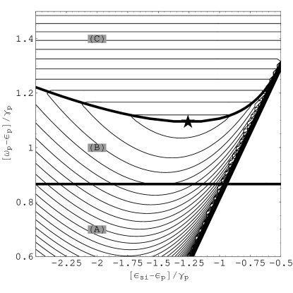
Figure 7: The same as Fig.5 for unequal damping rates $\gamma_{p}=\gamma_{s}=\gamma_{i}/5$. The lowest contour line in the plot is at $1.05I_{inc}^{min}$, where the minimum of the threshold intensity $I_{inc}^{min}$ is attained at the point indicated by a star $\star$. The difference between the contours is $0.1I_{inc}^{min}$.

In current experimental configurations, e.g. for a pump in the vicinity of the “magic angle”, the idler linewidth is often much larger than the signal and pump ones, i.e. $\gamma_{i}\gg\gamma_{p}\simeq\gamma_{s}$. Although the general formalism introduced in the previous sections keeps holding its validity, some of the physical conclusions of Sec.III.6 have to be modified. Because of the increased damping rate of the idler modes, the pump mode population $n_{xp}$ required by (10) for the onset of the parametric oscillation corresponds to a blue-shift of the pump mode $g|X_{p}|^{2}n_{xp}$ much larger than $\gamma_{p}$. With the frequency choice suggested by a naive application of the condition (15), the intensity value (18) would correspond to the end-point of the upper branch of the bistability curve. Unfortunately, this point can not be reached by the simple upward ramp of the pump laser intensity considered in the present paper, so that a more complete analysis is required which fully takes into account hysteresis effects.

The results are shown in Fig.7 for $\gamma_{p}=\gamma_{s}=\gamma_{i}/5$. Because of the high value of the pump mode blue shift at the onset of parametric oscillation, the (D) and (E) regions are shifted to large values of $\Delta_{p}$ (not shown), direct contact between the regions (A) and (C) is lost and the gap is filled by the (B) region. The optimal choice of the detunings lies on the border between the regions (B) and (C): parametric oscillation starts on the upper branch of the pump-only hysteresis curve exactly at the landing point of the jump from the lower branch. As one can see on Fig.7, the optimal values of the $\Delta_{p,si}^{opt}$ and $\Delta_{p}^{opt}$ detunings (measured in units of $\gamma_{p}$) are here larger than in the previous $\gamma_{p,s,i}=\gamma$ case. On the other hand, the threshold intensity is increased above the naive prediction (18) by a moderate factor of the order of two.

III.8 Quantitative discussion

In many technological applications of optical parametric oscillators, a value as low as possible for the threshold intensity can be a key advantage. In this respect, semiconductor microcavities in the strong coupling regime are very promising systems thanks to the extremely high value of the nonlinear coupling constant $g$, much higher than the one of OPOs based on passive $\chi^{(3)}$ media (see discussion below Eq. (4)).

Using typical values $\hbar\gamma=0.1-0.5\,\textrm{meV}$ for the damping rates and $N_{QW}=3$ for the number of quantum wells inside the cavity, Eq.(18) yields a value in the $0.13-3.2{\rm kW}/{\rm cm}^{2}$ range for the incident laser intensity at the parametric threshold, a value which is in rough agreement with experimental data of Refs. stevenson, ; houdre, ; baumberg, . Given the scaling relation (12), the threshold intensity of passive $\chi^{(3)}$ OPOs with a comparable quality factor is orders of magnitude higher. Unless planar cavities of much higher quality factor are developed to compensate for the much weaker nonlinearity of passive materials, semiconductor microcavities in the strong coupling regime appear to be most favourable systems in view of low-power OPO applications.

In order for this comparison to be fair and complete, it is important to extend it to the case of OPOs based on passive $\chi^{(2)}$ materials TROPO ; lugiato ; chi2OPO . In this case, no mean-field shift of the mode frequencies occurs and the minimum value of the parametric threshold is attained under the resonance condition $\omega_{p}=\epsilon_{si}$ and is equal to:

$$|P|_{min}=\gamma/(2g_{2}),$$ (19)

where the second-order nonlinear coupling constant for a planar cavity of thickness $d$ and filled of a medium of linear dielectric constant $\epsilon_{\rm lin}$ is

$$\hbar g_{2}=\mathcal{C}\chi^{(2)}\sqrt{\frac{(\hbar\omega_{p})^{3}}{\epsilon^{2}_{\rm lin}d}}.$$ (20)

At optimal pump detuning, the driving amplitude equals $|F_{p}|=\gamma\,|P|/2$, irrespective of the type of nonlinearity. Combining this result with eqns. (2), (4), (12), (19) and (20), one finds the ratio between the threshold laser intensities of $\chi^{(2)}$ and $\chi^{(3)}$ OPOs:

$$\frac{I^{(3)}_{min}}{I^{(2)}_{min}}=\frac{2\omega_{p}}{\gamma}\frac{[\chi^{(2)}]^{2}}{\chi^{(3)}}.$$ (21)

Using a typical value $\chi^{(3)}=10^{-9}\,\textrm{esu}$ for a large Kerr nonlinearity, the value $\chi^{(2)}=4\times 10^{-8}\,\textrm{esu}$ of the widely used KTP crystal NLO_mat , and $\gamma/\omega_{p}=2\times 10^{-4}$ as in a typical $\lambda/2$ semiconductor microcavity, the ratio (21) turns out to be around $0.016$.

This argument concludes the verification of the widespread expectation that for comparable values of the quality factor, the threshold intensity for parametric oscillation is orders of magnitude lower in semiconductor microcavities in the strong coupling regime than in OPOs based on passive $\chi^{(2,3)}$ materials.

IV Bifurcation type and nonlinear solution above threshold

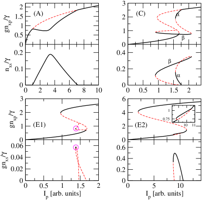
Figure 8: Pump and signal intensity as a function of the pump power in the different regimes. Black heavy full (red thin dashed) lines refer to the (un)stable solutions. $\gamma_{s,p,i}=\gamma$ are taken here, but the results are qualitatively robust to a change of the $\gamma$’s. Arbitrary units for $I_{p}$ are the same in all panels. (A) Optical limiter regime ($\omega_{p}-\epsilon_{p}=0,\epsilon_{si}-\epsilon_{p}=-1.5\gamma$); (C) Optical bistability regime where parametric and pump only threshold coincide ($\omega_{p}-\epsilon_{p}=1.5\gamma,\epsilon_{si}-\epsilon_{p}=-0.5\gamma$); (E1) Optical bistability regime where the parametric threshold precedes the pump only instability. The parametrically oscillating solution has a very small stable part ($\omega_{p}-\epsilon_{p}=1.5\gamma,\epsilon_{si}-\epsilon_{p}=0.4\gamma$); (E2) Same as E1, with a different set of parameters such that parametric oscillation is here possible for a wide range of pump intensities. ($\omega_{p}-\epsilon_{p}=3\gamma,\epsilon_{si}-\epsilon_{p}=2\gamma$). The inset shows a magnification of the pump population in the OPO regime.

In the previous section, our attention has been focussed on the behaviour of the system below the parametric threshold and we have characterized the value of the threshold intensity as a function of the detunings. To complete the study, it is then necessary to investigate the nature of the threshold point and characterize whether the onset of parametric oscillation takes place in a continuous or discontinuous way. Both kind of behaviours have been indeed observed in the experiments dasbach ; baumberg ; baas . Correspondingly, the theoretical analysis in the present section will show that a variety of different hysteresis effects can take place depending on the kind of bifurcation that occurs at the threshold. Again, our discussion here will be based on the assumption that ${\mathbf{k}}_{s,i}$ are given quantities. A complete discussion of the selection problem is postponed to a forthcoming publication pattern .

To make the analysis the simplest, a three-mode ansatz of the form:

$$\psi_{LP}({\mathbf{k}},t)=S\,\delta_{{\mathbf{k}},{\mathbf{k}}_{s}}e^{-i\omega_{s}t}+P\,\delta_{{\mathbf{k}},{\mathbf{k}}_{p}}e^{-i\omega_{p}t}+I\,\delta_{{\mathbf{k}},{\mathbf{k}}_{i}}e^{-i\omega_{i}t},$$ (22)

can be used whittaker01 ; whittaker05 , the signal/idler frequencies and wave vectors being related by $\omega_{i}=2\omega_{p}-\omega_{s}$ and ${\mathbf{k}}_{i}=2{\mathbf{k}}_{p}-{\mathbf{k}}_{s}$. By projecting the wave equation (1) onto the three signal, pump, and idler modes, the following equations of motion are found

$$i\frac{d}{dt}{\tilde{P}} = \left[\epsilon_{p}-i\frac{\gamma}{2}-\omega_{p}\right]\tilde{P}+g\,X_{p}^{2}\left[\left(|\tilde{P}|^{2}+2|\tilde{S}|^{2}+2|\tilde{I}|^{2}\right)\tilde{P}+2\tilde{P}^{\ast}\tilde{S}\tilde{I}\right]+\tilde{F}_{p}$$ (23)

$$i\frac{d}{dt}{\tilde{S}} = \left[\epsilon_{s}-i\frac{\gamma}{2}-\omega_{s}\right]\tilde{S}+g\,X_{s}^{2}\left[\left(2|\tilde{P}|^{2}+|\tilde{S}|^{2}+2|\tilde{I}|^{2}\right)\tilde{S}+\tilde{P}^{2}\tilde{I}^{\ast}\right]$$ (24)

$$i\frac{d}{dt}{\tilde{I}} = \left[\epsilon_{i}-i\frac{\gamma}{2}-2\omega_{p}+\omega_{s}\right]\tilde{I}+g\,X_{i}^{2}\left[\left(2|\tilde{P}|^{2}+2|\tilde{S}|^{2}+|\tilde{I}|^{2}\right)\tilde{I}+\tilde{P}^{2}\tilde{S}^{\ast}\right],$$ (25)

where the following shorthand notations have been introduced $\epsilon_{p,s,i}=\epsilon({\mathbf{k}}_{p,s,i})$ and $X_{p,s,i}=X({\mathbf{k}}_{p,s,i})$. Scaled quantities $\tilde{S}=X_{s}\,S$, $\tilde{P}=X_{p}\,P$, $\tilde{I}=X_{i}\,I$ and $\tilde{F}_{p}=X_{p}\,F_{p}$ have been also defined. Imposing the stationarity of the solution and the condition that $\omega_{s}$ is purely real gives a set of 7 real equations (3 complex ones, plus 1 real equation) which has to be solved for a total of 8 real quantities: the three amplitudes ${\tilde{S}},{\tilde{P}},{\tilde{I}}$ and the (complex) parametric oscillation frequency $\omega_{s}$. The extra degree of freedom which is left undetermined corresponds to the $U(1)$ signal/idler phase symmetry which is spontaneously broken above the threshold Goldstone .

Fig.8 shows the behaviour of the pump $n_{xp}=|\tilde{P}|^{2}$ and signal $n_{xs}=|\tilde{S}|^{2}$ mode occupations as a function of the incident pump intensity $I_{p}$ for different choices of pump laser $\omega_{p}-\epsilon_{p}$ and signal/idler detuning $\epsilon_{si}-\epsilon_{p}$. These plots exemplify the system behaviour in the most significant among the regimes studied in Fig.6. Full lines indicate stable regions, dashed lines are the unstable ones . Correspondingly, a numerical integration of the time-dependent equation of motion (23-25) has been performed for a laser intensity which is continuously swept up and down through the parametric threshold. The resulting time-dependence of $n_{xp}$ and $n_{xs}$ is shown in Fig.9 for the most significant cases.

Figure 9: Time evolution of the pump laser intensity (upper panels), pump intensity (central panels) and signal intensity (lower panels) for the same detuning parameters as in the panels A, C and E2 of Fig.8.

IV.1 Region (A): Optical limiter

In the optical limiter case of Fig.8A, both the pump and the signal mode occupations are continuous functions of the pump intensity. The transition is analogous to a second-order phase transition: the signal intensity is zero below and at the threshold and increases smoothly as a function of the pump power. In the language of nonlinear dynamics, this corresponds to a so-called supercritical Hopf bifurcation hale . The corresponding time evolution is shown in the plots in the left column of Fig.9: both $n_{xp}$ and $n_{xs}$ have a smooth evolution in time which is immediately understood by following the curves of Fig.8A. The kinks correspond to the points where parametric emission switches on and off.

It is interesting to compare this behaviour with the one of the $\chi^{(2)}$ OPO in the $\Delta_{0}\Delta_{1}<1$ regime discussed in Ref. lugiato, . As one can see in Figs.5 and 7, the optical limiter regime corresponds to $\epsilon_{si}-\epsilon_{p}<0$ and $\omega_{p}<\epsilon_{p}$. In both cases, the Hopf bifurcation is supercritical, and the populations are continuous functions of the pump intensity across the threshold. The behaviour well above the threshold is however completely different. In the $\chi^{(3)}$ case there is an upper threshold as well, so that parametric oscillation disappears for too large a pump intensity (not shown in the time-dependent plots). In the $\chi^{(2)}$ case, the parametric oscillation takes place instead for all values of the laser intensity above the threshold. As shown in Ref.lugiato, , for very high values of the incident intensity it becomes however unstable towards self-pulsing and chaotic behaviour.

The behaviour of the system for the parameters of Fig.6B is completely analogous to the optical limiter case: the pump only bistability and the parametric oscillation indeed take place in an independent way. In the OPO region, the behaviour of the pump and signal populations as a function of the incident intensity is therefore closely analogous to the one shown in Fig.8A.

IV.2 Region (C): Optical bistability

The physics turns out to be much richer whenever parametric oscillation and pump-only bistability take place in the same range of intensities. In the case shown in Fig.6C, the pump-only solution loses stability at the pump-only saddle node bifurcation. As the upper branch of the pump-only hysteresis loop is parametrically unstable, the parametric oscillation sets in. As shown in Fig.8C, the solution connecting the lower and upper threshold for OPO can be a complicate (multivalued) function whittaker05 : typically, there are two stable branches (indicated with $\alpha$ and $\beta$), which not always can be reached in a continuous way by means of a simple upward ramp of the pump intensity. To determine which branch is actually selected, the dynamics of the system has to be considered (central column of Fig.9). We have numerically found that the system jumps to the $\alpha$ branch as soon as the pump intensity exceeds the pump-only turning point. This $\alpha$ branch is then followed during both the upward and the following downward ramps until the saddle-node instability at the end of the branch is reached. At this point the system has to jump to another solution: our numerical simulations have shown that the $\beta$-branch is dynamically selected, where parametric oscillation still takes place with an even higher amplitude. Finally, when the saddle-node instability at the end of $\beta$ branch is reached, the system has no choice but to jump back to the lower branch of the pump-only solution where parametric emission is no longer present.

It is important to stress that this analysis is based on a three-mode approximation: although this is certainly a valid description of a three-mode cavity, it may be not representative of all that can happen in a many-mode system such as a planar microcavity, where the $\alpha$ branch is often Eckhaus-unstable against changes in the signal wavevector. On the other hand, the $\beta$ branch turns out to be generally much more stable. A more complete discussion of these issues will be presented in a forthcoming publication pattern .

IV.3 Regions (E1,E2): Optical bistability

In the E region, the parametric instability occurs before the pump-only one, and the corresponding Hopf bifurcation is generally of the subcritical type hale . Two subcases are to be distinguished.

For $\epsilon_{si}\gtrsim\epsilon_{p}$ (Fig.8E1), although the instability is of the parametric kind, no stable parametrically oscillating solution exists for any pump intensity above the threshold. The parametric threshold is in fact very close to the pump-only threshold, and only a very small part of the OPO solution is stable (circle in Fig.8). As this stable region corresponds to intensity values in between the upper and lower turning points of the pump-only bistability loop, parametric oscillation can not be reached by any continuous intensity ramp, no matter its direction.

For $\epsilon_{si}\gg\epsilon_{p}$ (Fig.8E2), the parametric threshold is instead sufficiently lower than the pump-only one for a stable OPO state to exist and to be reachable by means of an upward intensity ramp: a stable parametrically oscillating solution exists in fact for laser intensities extending from well below to well above the parametric instability threshold. However, as the bifurcation at the lower threshold is of the subcritical Hopf type, parametric oscillation sets in in a discontinuous way for an upward ramp in laser intensity. A time-dependent calculation is then needed to ensure that the system actually jumps from the lower branch of the pump-only hysteresis loop to the parametrically emitting solution rather than to the upper branch of the pump-only bistability loop. The results are shown in the right column of Fig.9: the switch-on of the OPO emission during the upward ramp is discontinuous, as well as the switch-off during the downward ramp. This latter corresponds to a saddle-node instability at a pump intensity slightly lower than the one of the subcritical Hopf instability. A new kind of hysteresis loop is therefore present: parametric emission gives in fact a positive feedback to the pump mode population and two solutions (a pump-only one and a parametrically emitting one) are possible in a range of pump intensity values. The main difference with respect to the standard pump-only hysteresis loop is that the higher turning point is here at a Hopf bifurcation rather than at a saddle-node one.

Remarkably, this phenomenology can be related to an analogous one shown by a $\chi^{(2)}$ OPO in the $\Delta_{0}\,\Delta_{1}>1$ regime of Ref.lugiato, . Indeed, $\omega_{p}>\epsilon_{p}$ and $\epsilon_{si}\gg\epsilon_{p}$ in our (E2) region. The qualitative shape of the parametrically-induced hysteresis loop is indeed similar, with the main difference of the hysteresis loop having a here a finite size also in the $n_{xp}$ vs. $I_{p}$ plot and not only in the $P$ vs. $I_{p}$ one. A qualitative analogy with the $\chi^{(2)}$ OPO can be found in the (C) case as well: in addition to the topological similarity, the pump mode population is a very flat function of $I_{p}$ along the $\beta$ branch, and the phase of the pump mode amplitude $P$ in the $\beta$ branch differs from the one in the lower branch of the bistability loop in a way very similar to the phase hysteresis shown in the $\Delta_{0}\Delta_{1}<1$ case of Ref.lugiato, .

IV.4 Considerations on quantum fluctuations

All the discussion so far has considered the polaritonic field as a classical one, and therefore has neglected its fluctuations around the mean-field value. Before concluding, it is interesting to shortly address the behaviour of the quantum fluctuations in the different cases. The fluctuations around the pump-only solution below the threshold are mostly determined by the nature of the instability at the threshold point, i.e. whether this is a single-mode or a parametric one. The physics of the fluctuations around the three-mode solution (22) above the threshold is instead more complex coh_length , and here we shall limit ourselves to a few, very general remarks.

In regions (A) and (B), the onset of parametric oscillation closely resembles a second-order phase transition: the signal, idler and pump mode populations have a continuous dependence on the pump laser intensity. The overall behaviour as a function of the pump laser intensity is qualitatively identical to the one discussed in Ref.iac-prb, as a function of the pump laser frequency: as the threshold point is approached from below, the magnitude of the quantum fluctuations of the signal and idler beam monotonically grows and eventually becomes very large in the vicinity of the threshold where an eigenvalue of the stability matrix (9) goes to zero. The fluctuations being due to parametric creation of signal-idler polariton pairs, the signal and idler beams show significant quantum correlation ciuti_OPA ; karr ; langbein_QC . Above the threshold, the signal and idler fields have a finite mean-field amplitude which continuously starts from zero. Quantum fluctuations around this three-mode mean-field solution have a more complex behaviour: a quite general fact is that the importance of the fluctuations is most important close to the threshold point, and then quickly decreases as one moves far from the threshold coh_length .

In the (E) cases, the behaviour is almost the same in the region below the threshold: the instability having a parametric nature, the quantum fluctuations (as well as the quantum correlations) in the signal and idler modes grow as the threshold is approached and become strongest in the close vicinity of the threshold point. On the other hand the behaviour above the threshold point is dramatically different: the onset of the parametric oscillation (provided it really starts, as in case E2) is discontinuous, and a completely different solution branch is selected (Fig.9E2). Furthermore, the landing point on the new branch is not necessarily in the vicinity of the end-point of the branch, so fluctuations are generally moderate. Yet, their magnitude becomes again large as one approaches the end-point of the branch where one eigenvalue of the stability matrix around the three-mode solution (22) tends to zero.

In the (C) case, the behaviour is very different already below threshold: as the instability at the end-point of the branch has a single-mode nature, the quantum fluctuations in the signal and idler modes remain moderate also in the vicinity of the threshold point, while the pump mode ones grow very large as typical of optical bistable systems w-m .

V Conclusions and outlook

In this paper we have given a systematic classification of the behaviour of a triply resonant optical parametric oscillator based on a semiconductor microcavity in the strong coupling regime. Because of the $\chi^{(3)}$ nature of the collisional excitonic nonlinearity, the interplay of optical bistability and optical parametric oscillation makes the behaviour of these systems much richer than the one of standard OPOs based on passive $\chi^{(2)}$ nonlinear materials, and a variety of different threshold behaviours can be found already within a simple three-mode theory. In agreement with recent experiments, depending on the specific value of the detunings, either a continuous switch-on or a discontinuous jump can be found for the behavior of the signal intensity at the parametric threshold. The different behaviours have been classified by means of the general theory of bifurcations, and a simple relation between the nature of the instability point and the behaviour of the quantum fluctuations at the threshold point has been pointed out.

In order to minimize the threshold incident intensity, a rigorous and quantitative refinement of the “magic angle” criterion is provided which takes into account the mean-field shift of the modes due to interactions, as well as the possibility of hysteresis effects in the pump-only dynamics. A slight blue-detuning of the pump laser and a comparable red-detuning of the signal/idler modes with respect to the pump mode frequency turns out to be favourable in order to compensate for the mean-field shift of the mode frequencies.

Generalization of the theory to the many-mode case is under way. In order to take fully into account the inhomogeneous spatial profile of the pump laser spot and the competition between parametric oscillation in different $k_{s}$ modes, techniques mutuated from the theory of pattern formation in nonlinear dynamical systems turn out to be of great utility.

- (1) P. D. Drummond, K. J. McNeil, and D. F. Walls, Opt. Acta 27, 321 (1980); P. D. Drummond, K. J. McNeil, and D. F. Walls, Opt. Acta 28, 211 (1981).
- (2) Special issue on optical parametric oscillation and amplification, J. Opt. Soc. Am. B 10, 1655 (1993).
- (3) R. M. Stevenson, V. N. Astratov, M. S. Skolnick, D. M. Whittaker, M. Emam-Ismail, A. I. Tartakovskii, P. G. Savvidis, J. J. Baumberg, and J. S. Roberts, Phys. Rev. Lett 85, 3680 (2000).
- (4) R. Houdré, C. Weisbuch, R. P. Stanley, U. Oesterle, and M. Ilegems, Phys. Rev. Lett. 85, 2793 (2000).
- (5) J.J. Baumberg, P. G. Savvidis, R. M. Stevenson, A. I. Tartakovskii, M. S. Skolnick, D. M. Whittaker, and J. S. Roberts, Phys. Rev. B 62, R16 247 (2000).
- (6) Special issue on Microcavities, edited by J. Baumberg and L. Viña [Semicond. Sci. Technol. 18, S279-S434 (2003)].
- (7) B. Deveaud (Ed.), Physics of semiconductor microcavities, Special issue of Phys. Stat. Sol. B 242, 2145-2356 (2005).
- (8) I. Carusotto and C. Ciuti, Phys. Rev. Lett. 93, 166401 (2004); C. Ciuti and I. Carusotto, Phys. Stat. Sol. (b) 242, 2224 (2005).
- (9) D.M. Whittaker, Phys. Rev. B 71, 115301 (2005).
- (10) D. Sanvitto, D. N. Krizhanovskii, D. M. Whittaker, S. Ceccarelli, M. S. Skolnick, and J. S. Roberts, Phys. Rev. B 73, 241308(R) (2006).
- (11) M. Wouters and I. Carusotto, in preparation.
- (12) D.M. Whittaker, Phys. Rev. B 63, 193305 (2001).
- (13) C. Ciuti, P. Schwendimann and A. Quattropani, Semicond. Sci. Techn. 18, S279 (2003) and references therein.
- (14) N. A. Gippius et al., Eur. Phys. Lett. 67, 997 (2004).
- (15) G. Dasbach, C. Diederichs, J. Tignon, C. Ciuti, Ph. Roussignol, C. Delalande, M. Bayer, and A. Forchel, Phys. Rev. B 71, 161308(R) (2005).
- (16) C. Richy, K. I. Petsas, E. Giacobino, C. Fabre and L. Lugiato, J. Opt. Soc. Am. B 12, 456 (1995).
- (17) M. Vaupel, A. Maître, and C. Fabre, Phys. Rev. Lett. 83, 5278 (1999); M. Martinelli, N. Treps, S. Ducci, S. Gigan, A. Maître, and C. Fabre, Phys. Rev. A 67, 023808 (2003).
- (18) L. A. Lugiato, C. Oldano, C. Fabre, E. Giacobino, and R. J. Horowicz, Nuovo Cimento 10D, 959 (1988).
- (19) I.A. Shelykh, A.V. Kavokin and G. Malpuech, Phys. Stat. Sol. 242, 2271 (2005).
- (20) W. Langbein, proceedings of ICPS 26 (Edinburgh, UK, 2002).
- (21) M.J. Collett and C.W. Gardiner, Phys. Rev. A 30, 1386 (1984).
- (22) C. Ciuti and I. Carusotto, cond-mat/0606554.
- (23) A. Baas, J.-Ph. Karr, M. Romanelli, A. Bramati and E. Giacobino, Phys. Rev. B 70, 161307(R) (2004).
- (24) C. Ciuti, V. Savona, C. Piermarocchi, A. Quattropani, and P. Schwendimann Phys. Rev. B 58, 7926 (1998).
- (25) M. Richard, J. Kasprzak, R. André, R. Romestain, L. S. Dang, G. Malpuech, and A. Kavokin, Phys. Rev. B 72, 201301(R) (2005).
- (26) For a discussion of disorder effects in disordered Bose systems at equilibrium, see e.g. M.P.A. Fisher, P.B. Weichman, G. Grinstein, and D.S. Fisher, Phys. Rev. B 40, 546 (1989).
- (27) R.L. Sutherland, Handbook of nonlinear optics (Marcel Dekker, 2003).
- (28) M. Wouters and I. Carusotto, preprint cond-mat/0512464.
- (29) A. Verger, C. Ciuti and I. Carusotto, Phys. Rev. B 73, 193306 (2006).
- (30) R. W. Boyd, Nonlinear optics (Academic Press, San Diego, 1992).
- (31) A. Baas, J.-Ph. Karr, H. Eleuch and E. Giacobino, Phys. Rev. A 69, 023809 (2004).
- (32) C. Ciuti, P. Schwendimann, and A. Quattropani, Phys. Rev. B 63, 041303(R) (2001).
- (33) J. Hale and H. Koçak Dynamics and Bifurcations (Springer-Verlag, New York, 1991).
- (34) M. Wouters and I. Carusotto, preprint cond-mat/0606755.
- (35) I. Carusotto and C. Ciuti, Phys. Rev. B 72, 125335 (2005).
- (36) C. Ciuti, P. Schwendimann, and A. Quattropani, Phys. Rev. B 63, 041303(R) (2001).
- (37) J.Ph. Karr, A. Baas and E. Giacobino, Phys. Rev. A 69 , 063807 (2004).
- (38) S. Savasta, O. Di Stefano, V. Savona, and W. Langbein, Phys. Rev. Lett. 94, 246401 (2005).
- (39) D. F. Walls and G. J. Milburn, Quantum Optics (Springer-Verlag, Berlin, 1994).