THE COLLISION CONSISTENCY OF LATTICE-BGK MODEL FOR SIMULATING RAREFIED GAS FLOWS IN MICROCHANNELS

Abstract

The collision consistency between the BGK collision model equation and lattice-BGK (LBGK) model is proposed by researching the physical significance of the relaxation factor $\tau$ in LBGK model. For microscalar flow in which the continuum hypothesis is not still satisfied, the collision consistency $\tau=1.0$ should be ensured when using the LBGK model for simulating microflows. The results of simulating microchannel Poiseuille flow with constant pressure gradient under collision consistency by using LBGK model are well consistent with the analytical solutions, and the accuracy of these results is three or four orders of magnitude higher than those that don’t satisfy the collision consistency.

PACS Nos.: 04.60.Nc, 47.45.-n, 47.61.-k

1 Introduction

Micro-electro-mechanical systems (MEMS) technology has been developed rapidly in recent years.[1]~[3] The characteristic length scale of MEMS is typically the order of microns, and the ratio of the mean free path to the characteristic dimension (i.e. Knudsen number $Kn$) can not be negligible. The dynamics associated with microchannels can thereby exhibit rarefied phenomena and compressibility effects. The former is the emergence of a slip velocity at the wall boundary in microchannel flows. The latter is the significant nonlinear pressure drop of gas flowing in a long microchannel. Because conducting experiments in micrometer-size is a big challenge, numerical simulations of MEMS become very important tools of investigation. But the methods commonly used in simulation of MEMS, such as molecular dynamics (MD), direct simulation Monte–Carlo (DSMC)[4] and direct numerical simulation of Boltzmann equation, usually requires a tremendous amount of computer time and memory. Recently, for its intrinsic kinetic nature, the Lattice Boltzmann method (LBE) has been become an attractive method for simulation of microscalar flows where both microscopic and macroscopic behaviors are coupled.[5, 6]

Form its birth nearly 20 years ago (1988)[7], the lattice Boltzmann method (LBM)[8]~[10] has met with significant success for the numerical simulation of a large variety of fluid flows, and has emerged as an alternative numerical technique for simulating fluid flows. The LBE method usually solves the Bhatnagar-Gross-Krook (BGK) model equation, a simplified model Boltzmann equation, on a discrete lattice, which is usually named the lattice-BGK (LBGK) model.[9, 10] Since theoretical connections between the LBGK model and the Boltzmann equation[11, 12] and the preliminary link between LBGK model and the Burnett-type equations[13] were established, the LBE model can be valid for rarefied gas flow provided the Mach number is small. Moreover, since the standard BGK equation is able to simulate highly non-equilibrium gas flows, the LBGK model should also be applicable to rarefied microflows theoretically.[14]~[20]

One of the most important issues of LBGK model for simulating microchannel flows is the introduction of $Kn$ number into LB models. The popular treatment is the construction of the relationship between $Kn$ and relaxation time $\tau$ of LB models. Nie et al. used the explicit LBE formulation and related the nondimensional relaxation time $\tau_{e}$ to Knudsen number $Kn$ as: $Kn=\alpha(\tau_{e}-0.5)/\rho H$ for a microchannel of height $H$ and gas density $\rho$. The factor 0.5 attributes to the explicit treatment of the collision term and $\alpha$ is chosen to best match the simulated mass flow rate with experiments.[14] Later, Lim et al.[15] proposed a different relation between $Kn$ and $\tau_{e}$ for the explicit LBE formulation without the correction factor of 0.5 as in Nie et al.. Their $Kn$ for a long microchannel was defined as $Kn=\left(\delta x\tau_{e}/H\right)/\left(p_{0}/p\right)$, where $p$ and $p_{0}$ are the local pressure and pressure at the outlet of the microchannel, respectively. Zhang et al. gave different definitions of $\tau_{e}$ with different constant factors among various lattice models.[18] Recently, Lee et al. proposed a definition of $\tau$ about fully implicit LBE.[19]

Another one is the implementation of boundary condition. Nie et al. used the half bounce-back rule for the slip effect at the surface. Lim et al. used a specular reflection model to generate slip effect. Zhang et al. adopted the Maxwellian scattering kernel to address the gas molecule and surface interactions with an accommodation coefficient $\alpha$. Lee et al. proposed a wall equilibrium condition according to the assumption of rough surface on the characteristic length of gas molecules.

For the former issue, the previous research is still related to the framework of Navier–Stokes equations. This is because the expression of the kinetic viscosity coefficient derived from the LB equation recovering the Navier–Stokes equations, is still adopted in the makeup of the relationship of $Kn$ and $\tau$. Furthermore, when $Kn$ approaches zero, the Boltzmann equation can be reduced to the Navier–Stokes equation. But all the existing LBE for microscale flow can not be reduced to the Navier–Stokes equation because of using the relationship between $Kn$ and $\tau$.

The previous researchers always focus on recovering the Navier–Stokes equations precisely from the LBGK model and ignoring the deviation of the LBGK model and Boltzmann equation. This deviation may not do any effect in simulation of macroscale flows. However, the character scale of microflows is much smaller. In such a case, keeping the collision consistency of the LBGK model and Boltzmann equation should be paid special attention. This collision consistency requires the collision frequency of LBGK model is equal to that of BGK model equation. With the further study on the relaxation factor $\tau$, we found that these two collision frequency are equivalent when $\tau=1.0$ and the simulation results are the most approximate. This principle is called collision consistency of LBGK model.

On the other hand, the boundary treatment is based on the Maxwell slip model straightforwardly. There is not any adjustable parameter in our model and is similar to the Newmann boundary condition in some degree. The implement is not related to the Navier–Stokes equations any more, so it can be applied in simulating microflows not only in slip regime but also in transition regime.

2 Lattice-BGK Equation and Collision Consistency

To begin with, the BGK equation is:

$$\frac{\partial h}{\partial t}+\textbf{c}\cdot\nabla h=-\frac{1}{\tau_{0}}\left(h-h^{eq}\right)$$ (1)

here $h=h(x,c,t)$ and $h^{eq}=h^{eq}(x,c,t)$ are the molecular distribution function and equilibrium distribution function, respectively.

$$h^{eq}=\frac{\rho}{m}\left(\frac{m}{2\pi k_{B}T}\right)^{D/2}\exp\left[-\frac{m(\textbf{c}-\textbf{u})^{2}}{2k_{B}T}\right]$$ (2)

where c and u are molecular velocity and macroscopical velocity respectively; $\tau_{0}$ is the collision time; $1/\tau_{0}$ represents the collision frequency: $1/\tau_{0}=\bar{c}/\lambda$. where $\bar{c}$ is molecular mean velocity; $\lambda$ is molecular mean free path.

LBGK model equation is:

$$\frac{\partial f_{i}}{\partial t}+\textbf{c}_{i}\cdot\nabla f_{i}=-\frac{1}{\tau_{0}}\left(f_{i}-f_{i}^{eq}\right)$$ (3)

here $f_{i}$ is particle distribution function:

$$f_{i}=\omega_{i}\left[1+\frac{(\textbf{c}_{i}\cdot\textbf{u})}{c_{s}^{2}}+\frac{(\textbf{c}_{i}\cdot\textbf{u})^{2}}{2c_{s}^{4}}-\frac{\textbf{u}^{2}}{2c_{s}^{2}}\right]$$ (4)

$\textbf{c}_{i}$ is lattice discrete velocity and $\omega_{i}$ is weighing factor, $\tau_{0}$ is the collision time.

LBGK equation (3) can be further discretized in space and time. The completely discretized form of Eq. (3), with the time step $\Delta t$ and space step $\Delta x=c_{i}\Delta t$, is:

$${f_{i}}(\textbf{x}+\textbf{c}_{i}\Delta{t},t+\Delta{t}) - {f_{i}}(\textbf{x},t)=-\frac{1}{\tau}\left[{f_{i}}(\textbf{x},t)-f_{i}^{eq}(\textbf{x},t)\right]$$ (5)

where x is a point in the discretized physical space, and it is worth notice that $\tau$ commonly considered as a nondimensional relaxation time, $\tau={\tau_{0}}/{\Delta t}$, represents the collision consistency of LBGK model by the analysis of the physical signification of $\tau_{0}$ and $\Delta t$.

The above discrete LBGK equation is usually solved in two steps: collision step and streaming step. So the physical process in LBGK model can be regarded as a large number of particles take place one collision, through the distance $\Delta x$ and the time $\Delta t$. Therefore, $\Delta x$ and $\Delta t$ can be regarded as the mean free path and the collision time in the LBGK model, respectively, and $1/\Delta t$ represents the collision frequency in the LBGK model. Consequently, $\tau={\tau_{0}}/{\Delta t}$ means the ratio of the collision frequency of the LBGK model to that of the BGK model. From the gas dynamics, the collision frequency $\tau_{0}$ is in direct proportion to the density, and in dependence on temperature, but independence of molecular velocity. In order to furthest approach to BGK model, the collision frequency of the LBGK model should be equal to that of the BGK model, i.e. $\tau={\tau_{0}}/{\Delta t}=1$. Especially in the microflows ($Kn>10^{-3}$), the collision consistency must be much more ensured for the collision frequency of molecule in the microflows is far lower than that in the macroscopical flows ($Kn<10^{-3}$).

It must be emphasized that LBGK model is between the BGK equation and Navier–Stokes equations. We formerly attached importance to recover the LBGK to Navier–Stokes equations in the simulation with LBGK model, but now we should pay sufficient attention to the consistency of the LBGK model with the BGK equation, especially in simulation of the microflows.

3 Knudsen Number, Lattice Number and Boundary Condition

In the LBGK model, $\Delta t$ is defined as:

$$\Delta t=\frac{\Delta x}{\textbf{c}}$$ (6)

and in the BGK model, $\tau_{0}$ is defined as:

$$\tau_{0}=\frac{\lambda}{\bar{c}}$$ (7)

Using Eq. (6) and Eq. (7), the relaxation factor $\tau$ can be determined as:

$$\tau=\frac{\Delta t}{\tau_{0}}=\frac{\bar{c}}{c}\frac{\Delta x}{\lambda}=\frac{c}{\bar{c}}\frac{1}{N_{H}Kn}$$ (8)

where $N_{H}$ is the number of the lattice in the characteristic length $H$, $H=\Delta xN_{H}$ .

Regarding $\bar{c}$ approximately equal to $c$[19], Eq. (8) can be simplified:

$$\tau=\frac{1}{N_{H}Kn}$$ (9)

According the collision consistency, the relation of $Kn$ to the number of the lattice is:

$$N_{H}=\frac{1}{Kn}$$ (10)

From Eq. (10), the number of lattice should be in inverse proportion to the Kn, rather than be determined randomly.

Under the collision consistency, Eq. (5) can be simplified as:

$${f_{i}}(\textbf{x}+\textbf{c}_{i}\Delta{t},t+\Delta{t})=f_{i}^{eq}(\textbf{x},t)$$ (11)

The distribution function $f_{i}$ evolved in the lattice actually is the equilibrium distribution function $f_{i}^{eq}$. Hence, if the velocity on the boundary can be determined, the distribution function of the boundary can also be determined.

To the slip flow regime, the macroscopical slip-velocity on the boundary can be obtained by:

$$u_{s}=\frac{2-\sigma}{\sigma}\lambda\left(\frac{\partial u}{\partial y}\right)_{wall}$$ (12)

where $u_{s}$ is the boundary slip-velocity; $\sigma$ is accommodation factor. Using second order difference formula, Eq. (12). Can be discretized as:

$$u_{s}=\frac{Kn\left(4u_{1}-u_{2}\right)}{2\Delta x+3Kn}$$ (13)

where $u_{1}$ and $u_{2}$ are the velocity of the first and the second point adjacent the wall, respectively.

4 Numerical Results and Discussion

In this paper, we study microscalar gas Poiseuille flows in a constant external pressure gradient in order to validate the collision consistency. The compressibility effect becomes negligible and only the rarefaction effect is accounted for. We study three cases with different $Kn$ number value ($Kn$=0.02, 0.05, 0.1), and the number of grids adopted in the simulations is chosen according to the collision consistency. Results will be compared with the analytical results and the results of more fine grids and relaxation factor chosen according to the Eq. (9).

4.1 Slip Flows

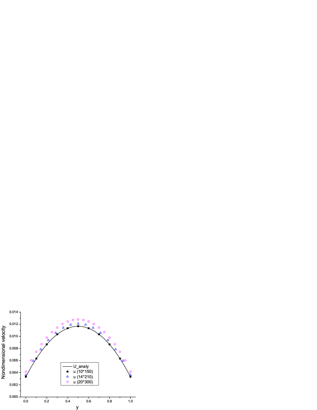
Figure 1: The comparison of velocity distribution of micro Poiseuille flow ($Kn=0.1$).

In case 1, when $Kn$=0.1, and the pressure gradient $dp/dx=6.6667\times 10^{-2}$. According to the collision consistency, relaxation factor $\tau=1.0$, and the grid numbers are $10\times 150$. From the calculating result (see Fig. 1), we can see the results agree closely with the analytical results when $\tau=1.0$, and the relative error is between $1.43-1.54\times 10^{-8}$. When $\tau=1/1.4$ and $\tau=0.5$, the fine grids are increased, but the simulative relative error is very big because of departing away from the collision consistency.

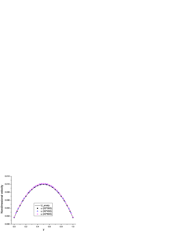
Figure 2: The comparison of velocity distribution of micro Poiseuille flow ($Kn=0.05$).

In Figure 2, when $Kn=0.05$ and the pressure gradient $dp/dx=6.6667\times 10^{-2}$, relaxation factor $\tau=1.0$ according to the collision consistency, we can see the simulating results agree closely with the analytical results, and the relative error is between $1.53-1.61\times 10^{-6}$. We increased the grids by 1.5 and 2 times and got the relaxation factor according to Eq. (9), but the relative error was still very large.

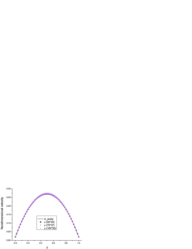
Figure 3: The comparison of velocity distribution of micro Poiseuille flow ($Kn=0.02$).

Figure 3 shows the comparison of calculating results obtained in different grids and relaxation factors when $Kn=0.02$ and the pressure gradient is 2.0. As can be seen from the graph, the results accord closely with the analytical results, but in the other two cases, the accuracy of the simulating results decreased instead of increasing although the grids increased 1.5 and 2 times, about four times less than that of when $\tau=1.0$.

The relaxation factors and relative calculation error in different situations. $Kn$ Grid $dp/dx$ Relaxation Relative error Relative error factor (Min) (Max) 0.10 $10\times 150$ $6.6667\times 10^{-2}$ 1.0 $1.43\times 10^{-8}$ $1.54\times 10^{-8}$ 0.10 $14\times 210$ $6.6667\times 10^{-2}$ 1/1.4 0.0362 0.0857 0.10 $20\times 300$ $6.6667\times 10^{-2}$ 0.5 0.0960 0.1020 0.05 $20\times 300$ $6.6667\times 10^{-2}$ 1.0 $1.53\times 10^{-6}$ $1.61\times 10^{-6}$ 0.05 $30\times 450$ $6.6667\times 10^{-2}$ 1/1.5 0.0120 0.0500 0.05 $40\times 600$ $6.6667\times 10^{-2}$ 0.5 0.0167 0.0750 0.02 $50\times 25$ 2.0 1.0 $2.38\times 10^{-6}$ $2.92\times 10^{-6}$ 0.02 $75\times 37$ 2.027 1/1.5 0.0021 0.0200 0.02 $40\times 600$ 2.0 0.5 0.0030 0.0300

All the calculating errors of different grids and relaxation factors in these three cases are shown in Table 1. For micro Poiseuille flow, the best calculating results are obtained since we adopted the relaxation factors in according to the collision consistency. So the simulating precision is 3 to 4 times more than that of the other results. From Table 1, we can see, the errors are almost the same under the same relaxation factors. This also illustrates the influence of the boundary error on the whole flow simulating error.

4.2 Higher $Kn$ Flows

We now investigate the simulation for higher $Kn$ number in this subsection. The ratio of the microchannel length $L$ to height $H$ is chosen as 100, and a 2000$\times$20 regular grid is applied, which has been verified by grid-dependence. We focus on the streamwise velocity profile $U$ at the exit normalized by the centerline maximum velocity and the pressure deviation $P^{\prime}=(p-p_{l})/p_{o}$ from the linear distribution $p_{l}=p_{o}+(p_{i}-p_{o})(1-x/L)$. Note that we choose the pressure deviation $P^{\prime}$ rather than the pressure distribution itself in order to show the difference more clearly.

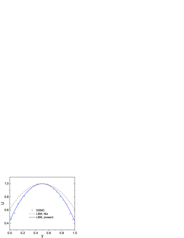
Figure 4: Normalized velocity profile at microchannel outlet ($Kn$=0.194).

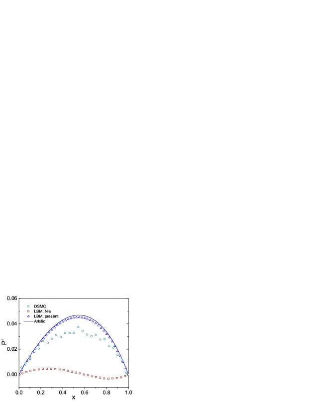
Figure 5: Pressure deviation $P^{\prime}$ along the microchannel ($Kn$=0.194).

Fig. 4 shows the velocity profile at the outlet of the microchannel with $Kn$=0.194. Compared with the reliable DSMC result, Nie et al. over-predicted the slip velocity obviously and the velocity distribution is more higher in nearly the whole outlet cross-section. In our simulation, both the slip velocity and exit velocity distribution are in consistent with the results of DSMC method. Moreover, pressure deviation $P^{\prime}$ is shown in Fig. 5. The qualitative difference with DSMC method has been founded in Nie et al.’s numerical result. Our present result is very closely to the analytical solution by Arkilic et al.. And the deviation from the DSMC result appears only in the middle part along the microchannels.

5 Conclusion

From our study, the physical meaning of the relaxation factor $\tau$ in LBGK model is: the ratio of the collision frequency in lattice system and in the BGK model. LBGK model situates between BGK model and macro Navier-Stokes equations so the collision consistency needs analyzing when LBGK model is dispersed from the BGK collision equation. This is very essential to adopting LBGK model to simulate the microflow because the continuum assumption may be break down in the microflow. Therefore we should assure the same collision frequency in LBGK model and BGK model, that is collision consistency.

Under collision consistency, it is simple to deal with the boundary and determine the relation factor. Adopting the collision consistency principle $\tau=1.0$, the results of the simulating Poiseuille flow accord closely with the analytical results. Without it, the precision of simulating results is three to four times less even if the greater grids are adopted.

References

- [1] C. M. Ho and Y. C. Tai, Annu. Rev. Fluid Mech. 30, 579 (1998).
- [2] D. J. Beebe, G. A. Mensing and G. M. Walker, Annu. Rev. Biomed. Eng. 4, 261 (2002).
- [3] G. E. Karniadakis and A. Beskok, Micro Flows: Fundamentals and Simulation (Springer, New York, 2001).
- [4] E. S. Oran, C. K. Oh and B. Z. Cybyk, Annu. Rev. Fluid Mech. 30, 403 (1998).
- [5] F. J. Higuera, S. Succi and R. Benzi, Europhys. Lett. 9, 345 (1989).
- [6] Y. H. Qian and S. A. Orszag, Europhys. Lett. 21, 255 (1993).
- [7] G. McNamara and G. Zanetti, Phys. Rev. Lett. 61, 2332 (1988).
- [8] R. Benzi, S. Succi and M. Vergassola, Phys. Report. 222, 145 (1992).
- [9] S. Chen and G. D. Doolen, Annu. Rev. Fluid Mech. 30, 329 (1998).
- [10] H. J. Liu, C. Zou, B. C. Shi, Z. W. Tian, L. Q. Zhang, and C. G. Zheng, Int. J. Heat Mass Tran. 49, 4672 (2006).
- [11] X. He and L. S. Luo, Phys. Rev. E 55, R6333 (1997).
- [12] X. Shan and X. He, Phys. Rev. Lett. 80, 65 (1998).
- [13] Y. H. Qian and Y. Zhou, Phys. Rev. E 61, 2103 (2000).
- [14] X. B. Nie and G. D. Doolen, J. Stat. Phys. 107, 279 (2002).
- [15] C. Y. Lim, C. Shu, X. D. Niu and Y. T. Chew, Phys. Fluids 14, 2299 (2002).
- [16] G. H. Tang, W. Q. Tao, and Y. L. He, Int. J. Modern Phys. C 15, 335 (2004).
- [17] X. D. Niu, C. Shu, and Y. T. Chew, Int. J. Modern Phys. C 16, 1927 (2005).
- [18] Y. Zhang, R. Qin and D. R. Emerson, Phys. Rev. E 71, 047702 (2005).
- [19] T. Lee and C. L. Lin, Phys. Rev. E 71, 046706 (2005).
- [20] Z. W. Tian, C. Zou, Z. H. Liu, Z. L. Guo, H. J. Liu, and C. G. Zheng, Int. J. Modern Phys. C 17, 603 (2006).