Contrasts between coarsening and relaxational dynamics of surfaces

Contrasts between coarsening and relaxational dynamics of surfaces Martin Siegert, Michael Plischke R.K.P. Zia The description of a number of surface relaxation processes in which the primary relaxation mechanism is diffusion of particles along the interface begins, in a continuum picture, with a Langevin equation of the form

$$\partial_{t}h({\bf r},t)+\nabla{\bf\cdot j}[h({\bf r},t)]=\eta({\bf r},t)$$ (1)

where ${\bf r}=(x_{1},x_{2})$ denotes the co-ordinates in a reference plane, $h$ is the height of the surface above it, ${\bf j}$ represents a surface diffusion current, and $\eta$ accounts for thermal noise. The conservation law in (1) reflects the assumed absence of voids, overhangs and evaporation of particles. For example, this equation was applied to the case of spinodal decomposition of an unstable crystal facet[2, 3]. In that case, $\nabla\cdot{\bf j}$ is simply the functional derivative of the surface free energy with respect to the function $h$.

Our interest here is another case: the growth of films by molecular beam epitaxy (MBE). It was realized some time ago[4, 5] that in MBE the breaking of detailed balance by the deposition process and the presence of step-edge barriers could lead to a nonequilibrium diffusion current that destabilizes a singular surface and leads to the formation of mounds or pyramids[6, 7]. This behavior is observed in simulations of discrete microscopic models as well as numerical integration of the following version of Eq. (1):

$$\partial_{t}h({\bf r},t) = -D\Delta\Delta h({\bf r},t)-v\Delta h({\bf r},t)$$ (3)

$$+u\sum_{\nu}\partial_{\nu}\left[\partial_{\nu}h({\bf r},t)\right]^{3}+\eta({\bf r},t)\ ,$$

where $\partial_{\nu}\equiv\partial/\partial x_{\nu}$, $\nu=1,2$, and $\Delta\equiv\partial_{1}^{2}+\partial_{2}^{2}$. The first term on the right arises from the equilibrium diffusion current[10], the next two represent the nonequilibrium diffusion current which with $v,\,u>0$ destabilize the singular surface ($\partial_{\nu}h=0$) and lead to a steady state composed of facets of slope $\partial_{\nu}h=\pm\sqrt{v/u}$. In particular, during the late stages, both methods reveal that these three-dimensional features coarsen as function of time with the characteristic length scale $R$ evolving as $t^{n}$ with $0.16\lesssim n\lesssim 0.25$. At present, this property is not

well understood.

In this letter, we focus on another aspect of the dynamics of this model, namely, relaxation into a steady state consisting of two domains. We also investigate an intimately related subject: the fluctuations of the interface separating these domains. Here, a domain refers to an area of constant slope mentioned above. For the analytic part, we will rely on Eq. (3), setting, for simplicity, $u=v=2D=1$. To compare with these results we will present data from both simulations and numerical integration of (3). Our main conclusion is that $z$, the exponent associated with relaxational dynamics, is 2. Specifically, we find that the relaxation time of a domain wall fluctuation of wavevector $k$ scales as $\tau_{k}\sim k^{-2}$. Thus, we have a system which violates $z=1/n$, a relation considered to be generic, coming from the dynamic scaling assumption with only a single time scale. Two well-studied systems obeying this relation are models A and B[11]. In the former, the Allen-Cahn equation[14] used to describe coarsening dynamics is even identical to the equation which describes the slowest relaxational mode[15], giving $z=1/n=2$. Similarly, the dynamics of model B is known to display a coarsening exponent $n=\frac{1}{3}$[12] and a relaxation exponent $z=3$[13]. In contrast to this simple situation, the behavior of our system is considerably richer and more intriguing. Not only do we find $z=2\neq 1/n$, we also observe the steady-state structure factor to scale as $S(k)\sim k^{-2}$. These results indicate that the coarsening process is controlled by defects that are not present in the stationary state.

It is tempting to compare our system with model B, both having similar non-linearities in the fields and conservation laws. However, there are serious differences, which are most apparent if we rewrite (3) in terms of a two-component “order parameter”, $m_{\nu}=\partial_{\nu}h$:

$$\partial_{t}m_{\nu}({\bf r},t) = -\hbox{$1\over 2$}\Delta\Delta m_{\nu}({\bf r},t)-\Delta m_{\nu}({\bf r},t)$$ (5)

$$+\sum_{\mu}\partial_{\nu}\partial_{\mu}\left[m_{\mu}^{3}({\bf r},t)\right]+\partial_{\nu}\eta({\bf r},t)\ ,$$

with the constraint $\partial_{\mu}m_{\nu}=\partial_{\nu}m_{\mu}$. By contrast, for a model B with two decoupled order parameters and a simple free energy density ${\cal F}=\sum_{\nu}\frac{1}{4}(\nabla m_{\nu})^{2}-\frac{1}{2}m_{\nu}^{2}+\frac{1}{4}m_{\nu}^{4}$, the third term would read $\Delta m_{\nu}^{3}$ and no constraint would be imposed on $m_{\mu}$.

We begin by discussing a stationary state with two domain walls. Such a state can be imposed on a system with substrate dimensions $L_{x}$, $L_{y}$ by screw boundary conditions in $x$: $h(x+L_{x},y)=h(x,y)+L_{x}$ and periodic ones in $y$: $h(x,y+L_{y})=h(x,y)$. Thus the average slope in $x$ can be unity, which is one of the preferred ground states. In the $y$-direction, there is a single ridge and a single valley and, except for two regions of characteristic size $\xi\approx\sqrt{2D/v}=1$, $\partial_{y}h(x,y)=\pm 1$. We denote the steady-state height function by $h_{c}(x,y)=x+\Phi_{c}(y)$ and its derivative with respect to $y$ by $\varphi_{c}(y)\equiv\partial_{y}h_{c}(x,y)=\Phi_{c}^{\prime}(y)$. Though $\Phi_{c}$ can be found exactly, its details will turn out to be unimportant. To provide the reader some familiar ground, we quote an example in the limit $\xi/L_{y}\to 0$: $\varphi_{c}(y)\to\tanh((y-l)/\xi)-\tanh((y-3l)/\xi)-1$, with $l=L_{y}/4$, where the valley and ridge are located at $y=l$ and $y=3l$, respectively.

Assuming now that $h({\bf r},t)=h_{c}({\bf r})+\chi({\bf r},t)$ and linearizing (3), we find that $\chi$ satisfies the Langevin equation

$$\partial_{t}\chi({\bf r},t)=-{\cal L}\chi({\bf r},t)+\eta({\bf r},t)$$ (6)

with the Hermitian operator ${\cal L}=\frac{1}{2}\Delta\Delta-\partial_{x}[V(\partial_{x}h_{c})\partial_{x}]-\partial_{y}[V(\partial_{y}h_{c})\partial_{y}]$ and $V(\zeta)=3\zeta^{2}-1$. The fluctuations of the surface can thus be expanded

$$\chi({\bf r},t)=\sum_{\ell}A_{\ell}(t)v_{\ell}({\bf r})\ ,$$ (7)

in terms of the eigenfunctions $v_{\ell}$ which solve the eigenvalue problem

$${\cal L}v_{\ell}({\bf r})=\lambda_{\ell}v_{\ell}({\bf r})=\lambda_{n}(q)\psi_{n}(q,y)e^{-iqx}\ .$$ (8)

Note that, for the last equality, we have exploited the translational invariance in $x$.

There are several branches of the eigenvalue spectrum. Two of these, the height fluctuation modes and the ‘Goldstone’ branch, terminate at $q=0$ with eigenvalue zero. The eigenfunctions of these zero-frequency modes are simply $\psi_{H}(0,y)=1$ and $\psi_{G}(0,y)=\varphi_{c}(y)$. The result $\lambda_{H}(q=0)=0$ follows from translational invariance in $h$, while $\lambda_{G}(q=0)=0$ is due to Goldstone’s theorem. The higher modes of the H-branch are simply obtained: $\psi_{H}(q,y)=\exp(iqx)$ with $\lambda_{H}(q)=2q^{2}+q^{4}/2$. The nontrivial G-modes, on the other hand cannot be determined exactly. Focusing on small $q$, we write ${\cal L}={\cal L}_{0}+{\cal V}(q)$ with ${\cal V}(q)=q^{2}(2-\partial_{y}^{2}+q^{2})$ as a perturbation. Perturbation theory or the variational method

$$\lambda\leq\int dy\,\varphi{\cal L}\varphi\biggl{/}\int dy\,\varphi^{2}$$ (9)

with a trial function $\varphi=\varphi_{c}$ both yield $\lambda_{G}(q)=2q^{2}+{\cal O}(q^{2}/L_{y},q^{4})$.

Finally, a third set of low-lying modes can be identified — the breathing modes in which the ridge and valley move in opposite directions. An appropriate choice of the variational eigenfunction in (9) for the breathing mode is $\psi_{B}(0,y)\simeq\tanh(y-l)+\tanh(y-3l)-y/l+2$ where the last two terms guarantee that the integral of this function is zero and that periodic boundary conditions are satisfied. A simple calculation using $\psi_{B}^{\prime}(y)\simeq|\psi_{G}^{\prime}(y)|-1/l$ then produces the bound $\lambda_{B}(q=0)\leq 96/L_{y}^{2}$. It is also easy to see that higher modes have the property $\lambda_{B}(q)=c/L_{y}^{2}+2q^{2}+{\cal O}(q^{2}/L_{y},q^{4})$ with some numerical constant $c\leq 96$. Thus, the breathing mode has a gap $\sim 1/L_{y}^{2}$. However, for quadratic systems ($L_{x}=L_{y}$) this gap is of the same order as $q^{2}$ and therefore $\lambda_{B}$ is of the same order as $\lambda_{G}$ for nonzero $q$. Thus, all eigenvalues that we have found so far scale in lowest order as $\lambda_{n}(q)\sim q^{2}$. For an exactly solvable version of this model[16] it is found that this statement is indeed correct for all eigenvalues. Perhaps $\lambda\sim q^{2}$ should not be a surprise, considering the presence of at least two gradients on the RHS of (3) or (5). This is also the case, for a homogeneous state, in model B. The contrast with model B becomes dramatic only when we consider inhomogeneous states, which admit Goldstone modes. In model B, the fact that ${\cal L}$ is not Hermitian leads to $\lambda\sim q^{3}$[13] while here $\lambda\sim q^{2}$.

We now can calculate two-point correlation functions such as $S({\bf k,}\tau)\equiv\int d^{2}r^{\prime}d^{2}r\,e^{i{\bf k\cdot r}}\left\langle\chi({\bf r}^{\prime},t)\chi({\bf r}^{\prime}+{\bf r},t+\tau)\right\rangle$. Expanding the noise $\eta$ in terms of the eigenfunctions, we write $\eta({\bf r},t)=L_{x}^{-1/2}\sum_{n,q}B_{n}(q,t)\psi_{n}(y)e^{-iqx}$. Using Eqs. (6), (7) and $\langle\eta({\bf r},t)\eta({\bf r}^{\prime},t)\rangle=2\epsilon\delta({\bf r}-{\bf r}^{\prime})\delta(t-t^{\prime})$, we find

$$S({\bf k},\tau)=\sum_{n}{\frac{\epsilon}{\lambda_{n}(q)}}\widehat{\psi}_{n}(p)\widehat{\psi}_{n}(-p)e^{-\lambda_{n}(q)\tau}\ ,$$ (10)

where ${\bf k}\equiv(q,p)$ and $\widehat{\psi}_{n}(p)$ is the Fourier transform of the (normalized) $\psi_{n}(y)$. This is a general result, showing that the term associated with the lowest eigenvalue will dominate the sum as $\tau\rightarrow\infty$. However, in our case, there is no gap, i.e., all $\lambda$’s are ${\cal O}(1/L^{2})$, so that there is no valid reason to keep only one or two terms. Because of the dependence on the Fourier transforms of the eigenfunctions, $S(q,p,\tau)$ will not display simple scaling, apart from the special case $p=0$. However, since all eigenvalues are proportional to $k^{2}$ the time-time correlation function $\Phi({\bf k},\tau)=S({\bf k},\tau)/S({\bf k},0)$ depends only on $k^{2}\tau$ and thus the dynamic exponent that governs the fluctuations in the steady state is $z=2$.

We are also interested in the interface structure factor $S_{I}(q,\tau)$ as it may provide more insight into the coarsening behavior. The position of the interfaces is determined by the condition $\partial_{y}h(x,y,t)=0$. This equation has two solutions $y_{1}(x,t)$ and $y_{2}(x,t)$ that correspond to the positions of the top and the valley of the height profile. The interface structure factor can be calculated using either of the two functions, $S_{I}(q,t)=\langle\widehat{y}_{1}(q,t+\tau)\widehat{y}_{1}(-q,t)\rangle=\langle\widehat{y}_{2}(q,t+\tau)\widehat{y}_{2}(-q,t)\rangle$. In linear approximation we find that $y_{1}(x,t)=-\partial_{y}\chi({\bf r},t)/\partial_{y}^{2}h_{c}(y)|_{y=l}$, and therefore

$$S_{I}(q,\tau) = {1\over[h^{\prime\prime}_{c}(l)]^{2}}\langle\widehat{\partial_{y}\chi}|_{y=l}(q,t+\tau)\widehat{\partial_{y}\chi|}_{y=l}(-q,t)\rangle$$ (11)

$$= {1\over[h^{\prime\prime}_{c}(l)]^{2}}\sum_{n}[\partial_{y}\psi_{n}(l)]^{2}{\epsilon\over\lambda_{n}(q)}e^{-\lambda_{n}(q)\tau}\ .$$ (12)

Because of the symmetries of the steady-state configurations all eigenfunctions are either symmetric or antisymmetric about $y=0$ and $y=l$. Of these four classes, only eigenfunctions that have a nonzero derivative at $y=l,3l$ contribute to $S_{I}(q,t)$ (12). The most important modes with this property are the Goldstone mode $\psi_{G}(y)$ and the breathing mode $\psi_{B}(y)$. Since $\partial_{y}\psi_{G}|_{y=l},\partial_{y}\psi_{B}|_{y=l}\sim L_{y}^{-1/2}$ we therefore find

$$S_{I}(q,\tau)={\epsilon\over L_{y}}\left[{c_{G}\over\lambda_{G}(q)}e^{-\lambda_{G}(q)\tau}+{c_{B}\over\lambda_{B}(q)}e^{-\lambda_{B}(q)\tau}+\ldots\right]\ ,$$ (13)

where $c_{G}$ and $c_{B}$ are numeric constants. Hence the interfaces fluctuations are governed by a dynamic exponent $z=2$ as well. Furthermore, Eq. (13) shows that the interface structure factor scales as $S_{I}(q)\sim 1/(q^{2}L_{y})$. A major consequence is that the interface width, $w(t)=[L_{x}^{-1}\int dx\,y_{1}^{2}(x)]^{1/2}\sim[L_{x}/L_{y}]^{1/2}$, does not diverge in the thermodynamic limit (provided $L_{x}\sim L_{y}$). Hence the pyramids that form in the coarsening dynamics are separated by flat interfaces in striking contrast to the interfaces in models A or B, in which the widths diverge as $\sqrt{L}$.

The coarsening dynamics of Eqs. (1) and (5) are still not well understood. Recently, Rost and Krug[17] presented a scaling theory of coarsening for the rotationally invariant current ${\bf j}_{\rm iso}={\bf m}(m_{0}^{2}-m^{2})$ that neglects the crystalline symmetries of the growing film. It is questionable whether such scaling theories are correct. The growth law for the average domain size depends usually on two lengthscales: the average domain size $R(t)$ itself and the width of the domain walls $\xi$. This was made clear by Bray and Rutenberg[18]. For the Cahn-Hilliard equation $\partial_{t}m=-\Delta[\Delta m+m(1-m^{2})]$ they find that the domains grow as $\dot{R}(t)\sim 1/[\xi R^{2}(t)]$ leading to a coarsening exponent $n=1/3$. Scaling and mean-field-like theories[20] for the Cahn-Hilliard equation yield $n=1/4$. This result is obtained, if the assumption is made that there is only one relevant lengthscale, the average domain size, so that $\xi$ is replaced by $R(t)$ in the expression above. Since the dimensionality of the operators in Eq. (5) is the same as those of the Cahn-Hilliard equation, scaling theories and dimensional analysis for equation (1) with a current ${\bf j}\neq{\bf m}f(|{\bf m}|)$ are not very convincing. For the case of an isotropic current as studied in Ref. [17] the situation seems to be not so bad: At least in the analogous case of the Cahn-Hilliard equation only logarithmic corrections to the growth law are found[18] if compared with scaling theories.

Rost and Krug[17] assume that the average slope approaches the limiting value $m_{0}$ in a power law manner, $\langle m\rangle=m_{0}-ct^{-\alpha^{\prime}}$, and they find that the exponent $\alpha^{\prime}$ is linked to the coarsening exponent through $\alpha^{\prime}=2n$. For model B the corresponding relation is different; the order parameter approaches its limiting value as $m_{0}-m(t)\sim t^{-1/3}$. Nevertheless, our calculations do lend some support for the relation $\alpha^{\prime}=2n$ even in the case of an anisotropic surface current. A central result of our study is that all modes are gapless, $\lambda({\bf k})\sim k^{2}$. Consequently, slope fluctuations decay like $(\delta m(t))^{2}\sim\int d^{2}r[\partial_{x}\chi({\bf r},t)]^{2}\sim t^{-1/2}$ and therefore $\alpha^{\prime}=1/2$. Hence the relation $\alpha^{\prime}=2n$ yields $n=1/4$ in agreement with numerical solutions[7, 19] of Eq. (3). Therefore, the differences between model B and surface dynamics that became apparent in the calculations presented above, in particular the fact that $n\neq z^{-1}$, may also be responsible for the difference in the growth law.

We now discuss numerical calculations that verify the properties derived above. We have integrated Eq. (3) and also carried out Monte Carlo simulations for a discrete growth model [21]. Both display the same kind of instability and coarsening behavior. In the latter, particles are randomly deposited on an initially flat substrate and the growing cluster relaxes by surface diffusion. An instability is produced by step-edge barriers in one of the two hopping directions on the square lattice. The steady state for a finite system is then a single mound with its ridge and valley perpendicular to this axis. In Fig. 1 we show the static structure factor $S_{I}(q)$ for the ridge for three different

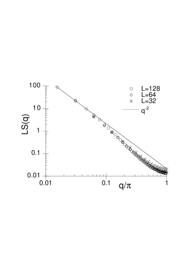
FIG. 1.: The static structure factor for interface fluctuations in a model of MBE that is unstable toward mound formation [21] for substrate sizes $L_{x}=L_{y}=$ 32, 64, 96 obtained from Monte Carlo simulations. Parameters are as given in [21]. Note that the data collapse only if $S(q)$ is multiplied by the substrate size $L$.

substrate sizes with $L_{x}=L_{y}=L$. The collapse of the data, when $S_{I}(q)$ is multiplied by $L$ is quite impressive. Further, the data seem to be converging to the $q^{-2}$-dependence predicted above.

In Fig. 2 we show the relaxation functions

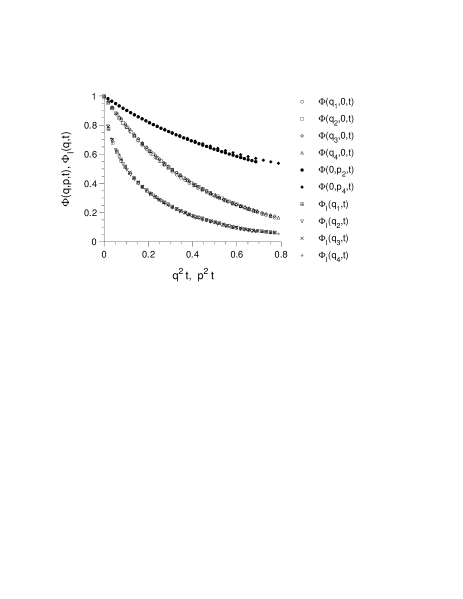
FIG. 2.: Relaxation functions $\Phi(q,p,t)$ and $\Phi_{I}(q,t)$ obtained from a numerical integration of Eq. (3) as a function of the scaled arguments $q^{2}t$ and $p^{2}t$, $q_{n}=2\pi n/L_{x}$ and $p_{n}=2\pi n/L_{y}$, $L_{x}=L_{y}=192$.

$\Phi(q,p,t)\equiv S(q,p,t)/S(q,p,0)$ and $\Phi_{I}(q,t)\equiv S_{I}(q,t)/S_{I}(q,0)$ obtained by integration of Eq. (3). The data collapse perfectly to single curves when plotted as a function of $q^{2}t$, $p^{2}t$ respectively, in complete agreement with (10) and (13). The only exceptions are the modes $S(0,p_{n},t)$ with $p_{n}=2\pi n/L_{y}$ and $n$ an odd integer. For these modes, the difference of two large quantities is encountered and we have not succeeded in obtaining the necessary statistical and numerical accuracy to reach a definitive conclusion. More details of our study, including tests for the $L_{y}$ dependence using rectangular lattices, will be presented elsewhere[16].

In summary, we have demonstrated both by analytic calculations and by simulations that this class of nonequilibrium processes behaves quite differently from models A and B. In particular, the exponent $z$ that controls the relaxation of interface fluctuations in the steady state is not related to the coarsening exponent $n$ by $n=1/z$. While this is interesting in its own right, it also indicates that a theory of coarsening for these processes must be based on the interactions of more complicated defects than those allowed in the steady state. However, if the exponent relation $\alpha^{\prime}=2n$[17] is used, our result $z=2=1/\alpha^{\prime}$ yields a coarsening exponent $n=1/4$.

The results derived in this letter are also relevant for the interpretation of experimental results obtained, e.g., in scattering experiments of films grown using MBE. If the surface evolution can be described by pyramid formation and coarsening, one expects that the scattering amplitude has a “ring” structure[22], i.e., a maximum at finite wavevectors ${\bf k}_{{\rm max}}(t)\sim 1/R(t)\sim t^{-n}$. However, once $k_{\rm max}$ becomes smaller than the minimum resolvable wavelength, the observed scattering is due to fluctuations of a single pyramid. In that case, the dynamic exponent $z=2$ as explained above. Moreover, the measured roughness exponent $\alpha$ then also characterizes fluctuations superimposed on the pyramid structure and has the value $\alpha=0$. Experimentally, it may be very difficult to detect this logarithmic roughness.

This research was supported by the NSERC of Canada and the US National Science Foundation through the Division of Materials Research. One of us (RKPZ) is grateful for the hospitality of M. Wortis and the physics department of Simon Fraser University.

REFERENCES

- [1]
- [2] J. Stewart and N. Goldenfeld, Phys. Rev. A 46, 6505 (1992).
- [3] F. Liu and H. Metiu, Phys. Rev. B 48, 5808 (1993).
- [4] J. Villain, J. Phys. I (France) 1, 19 (1991).
- [5] J. Krug, M. Plischke, and M. Siegert, Phys. Rev. Lett. 70, 3271 (1993).
- [6] M. D. Johnson, C. Orme, A. W. Hunt, D. Graff, J. Sudijono, L. M. Sander, and B. G. Orr, Phys. Rev. Lett. 72, 116 (1994).
- [7] M. Siegert and M. Plischke, Phys. Rev. Lett. 73, 1517 (1994).
- [8] H.-J. Ernst, F. Fabre, R. Folkerts, and J. Lapujoulade, Phys. Rev. Lett. 72, 112 (1994); J.E. Van Nostrand, S.J. Chey, M.-A. Hasan, D.G. Cahill, and J.E. Greene, Phys. Rev. Lett. 74, 1127 (1995).
- [9] J. A. Stroscio, D. T. Pierce, M. Stiles, A. Zangwill, and L.M. Sander, Phys. Rev. Lett. 75, 4246 (1995); C. Orme, M. D. Johnson, K. T. Leung, and B. G. Orr, Mater. Res. Soc. Symp. Proc. 340, 233 (1994); K. Thürmer, R. Koch, M. Weber and K. H. Rieder, Phys. Rev. Lett. 75, 1767 (1995); W. C. Elliott, P. F. Miceli, T. Tse and P. W. Stephens, Proceedings of the NATO ASI on Surface Diffusion: Atomistic and Collective Processes, Rhodes, Greece (1996), to be published.
- [10] W. W. Mullins, J. Appl. Phys. 28, 333 (1957); in Metal Surfaces: Structure, Energetics and Kinetics (Am. Soc. Metals, Metals Park, Ohio 1963).
- [11] P. C. Hohenberg and B. I. Halperin, Rev. Mod. Phys. 49, 435 (1977).
- [12] I. M. Lifshitz and V. V. Slyozov, J. Phys. Chem. Solids 19, 35 (1961); C. Wagner, Z. Elektrochem. 65, 581 (1961); T. M. Rogers, K. R. Elder and R. C. Desai, Phys. Rev. B 37, 9638 (1988); for an overview on ordering dynamics see A. Bray, Adv. Phys. 43, 357 (1994).
- [13] J. S. Langer and L. A. Turski, Acta Metall. 25, 1113 (1977); D. Jasnow and R. K. P. Zia, Phys. Rev. A 36, 2243 (1987); R. Bausch, R. Kree, A. Lusakowski, and L. A. Turski, Int. J. Mod. Phys. B 2, 1537 (1988).
- [14] S.M. Allen and J. W. Cahn, Acta Metall. 27, 1085 (1979).
- [15] R. Bausch, C. Dohm, H. K. Janssen, and R. K. P. Zia, Phys. Rev. Lett. 47, 1837 (1981).
- [16] R. K. P. Zia, M. Siegert, and M. Plischke, to be published.
- [17] M. Rost and J. Krug, preprint cond-mat/9611206 (1996).
- [18] A. J. Bray and A. D. Rutenberg, Phys. Rev. E 49, R27 (1994).
- [19] M. Siegert, in Scale Invariance, Interfaces, and Non-Equilibrium Dynamics, edited by A. J. McKane, M. Droz, J. Vannimenus, and D. Wolf, NATO ASI Series B, Vol. 344 (Plenum, New York, 1995), pp. 165-202.
- [20] see, e.g., G. F. Mazenko, O. T. Valls, and M. Zannetti, Phys. Rev. B 38, 520 (1992).
- [21] M. Siegert and M. Plischke, Phys. Rev. E 53, 307 (1996).
- [22] The word “ring” should not be taken literally, because the anisotropies of the lattice structure will also be seen in the ring structure.