First-principles theory of structural phase transitions for perovskites: competing instabilities

Abstract

We extend our previous first-principles theory for perovskite ferroelectric phase transitions to treat also antiferrodistortive phase transitions. Our approach involves construction of a model Hamiltonian from a Taylor expansion, first-principles calculations to determine expansion parameters, and Monte Carlo simulations to study the resulting system. We apply this approach to three cubic perovskite compounds, SrTiO₃, CaTiO₃, and NaNbO₃, that are known to undergo antiferrodistortive phase transitions. We calculate their transition sequences and transition temperatures at the experimental lattice constants. For SrTiO₃, we find our results agree well with experiment. For more complicated compounds like CaTiO₃ and NaNbO₃, which can have many different structures with very similar energy, the agreement is somewhat less satisfactory.

I Introduction

Perovskite materials are of considerable interest both for fundamental reasons and for their many actual and potential technological applications. The great fascination of the cubic perovskite structure is that it can readily display a variety of structural phase transitions, ranging from non-polar antiferrodistortive (AFD) to ferroelectric (FE) and antiferroelectric (AFE) in nature.[1] The competition between these different instabilities evidently plays itself out in a variety of ways, depending on the chemical species involved, leading to the unusual variety and richness of the observed structural phase diagrams. For example, as temperature is reduced, BaTiO₃ undergoes a series of FE phase transitions, while SrTiO₃ has a single AFD transition. More extreme examples are NaNbO₃ and BaZrO₃; the former has a series of six transitions, while the latter stays cubic down to zero temperature. Another appealing property of these cubic perovskites is that all of the structural phase transitions involve only small distortions from the ideal cubic structure, the typical distortion being less than 5% of the lattice constant. This simplifies the theoretical treatment considerably. The ample experimental data on these compounds also provide many insights and opportunities for checking the accuracy of theoretical calculations.

It is no wonder that there have been many theoretical attempts to study these compounds. Previous phenomenological model Hamiltonian approaches[2, 3, 4, 5] have largely been limited by oversimplification and ambiguities in interpretation of experiment, while empirical [6] and non-empirical pair-potential methods [7] have not offered high enough accuracy. Recently, advances in density-functional techniques have made possible first-principles investigations of such perovskite compounds. Such calculations have proven capable of providing accurate structural properties and FE distortions for perovskites at zero temperature.[8, 9, 10]

Recently, a thermodynamic theory based upon such first-principles calculations was developed to study the finite-temperature properties of BaTiO${}_{3},$[11, 12] and predicted the correct transition sequence and fairly accurate transition temperatures. This thermodynamic approach involves three steps: (i) constructing an effective Hamiltonian to describe the important degrees of freedom of the system; (ii) determining all the parameters of this effective Hamiltonian from high-accuracy ab-initio LDA calculations; and (iii) performing Monte Carlo simulations to determine the phase transformation behavior of the resulting system. A similar approach was also successfully applied to PbTiO₃ by Rabe and Waghmare.[13]

The construction of the effective Hamiltonian is carried out in view of the special structure properties of cubic perovskite compounds. At higher temperature, the cubic perovskite compounds ABO₃ have a simple cubic structure with O atoms at the face centers and metal atoms A and B at the cube corner and body center, respectively. The two most common instabilities result from the softening of either a polar zone-center phonon mode, leading to a FE phase, or the softening of a non-polar zone-boundary mode involving rotations of oxygen octahedra, leading to an AFD phase. (In some cases a zone-boundary polar mode may also occur, leading to an AFE phase.) In our previous thermodynamic theory for BaTiO₃, we assumed FE and strain distortions would be the only important degrees of freedom of the system. In other words, all other distortions are assumed to be much higher in energy. This is true for BaTiO₃, but not true for cubic perovskites in general. As shown in our recent first-principle calculations,[14] most cubic perovskite compounds may also undergo AFD transitions. To study these compounds, we need to extend our theory to include AFD distortions among the low-energy distortions. This extended theory would also allow us to study the interaction between FE and AFD instabilities. However, because the AFD distortion is a zone-boundary distortion without a clear corresponding zone-center mode, the extension is not trivial.

The rest of the paper is organized as follows. In Sec. II, we go through the detailed procedure for the construction of the effective Hamiltonian with the AFD distortion included. In Sec. III, we describe our first-principles calculations and the determination of the expansion parameters for the three compounds SrTiO₃, CaTiO₃, and NaNbO₃. In Sec. IV, we report our calculated transition temperatures, phase sequences, and order parameters for those three compounds. We also identify the differences between the correlation functions of the FE and AFD local modes in SrTiO₃. Sec. V concludes the paper.

II Construction of the Hamiltonian

A Local modes for AFD distortion

In our previous development,[12] we argued that the total energy of a cubic perovskite can be well approximated by a low-order Taylor expansion over all the relevant low-energy distortions, specifically FE distortions and strain. The FE distortions are represented by local modes, whose arrangement will reproduce the FE soft phonon modes throughout the Brillouin zone (BZ). To extend the theory to include the AFD distortions, we need to construct a new set of local modes to represent the lowest AFD modes over the whole BZ, or at least over the portion of the BZ where the energy change due to the AFD distortions is either negative, or positive but small. The AFD mode typically has the lowest energy at the zone-boundary R (0.5, 0.5, 0.5)$2\pi/a_{0}$ and M [(0.5, 0.5, 0)$2\pi/a_{0}$, etc.] points, while near the zone center $\Gamma$ the energy is very high. So it is necessary to choose local modes that will accurately reproduce the potentially soft modes in the vicinity of the R and M points.

The rotation of an isolated oxygen octahedron can be represented by a pseudovector passing through its center. Assuming the origin of coordinates at the center of the octahedron, a pseudovector with polarization $\hat{\bf z}$ involves displacements $\pm 0.5a_{0}\hat{\bf y}$ for oxygen atoms at ($\pm a_{0}$/2,0,0) and displacements $\mp 0.5a_{0}\hat{\bf x}$ for atoms at (0,$\pm a_{0}$/2,0). Here $a_{0}$ is the lattice constant of the ideal cubic perovskite. In the case of the ABO₃ perovskite crystal, we can represent octahedral rotation using pseudovectors sitting on the center of each octahedron, i.e., on the B atoms. However, neighboring octahedra share oxygen atoms, so that some continuity conditions would have to be imposed if we were to insist that the displacement of a given oxygen be consistently described by both neighboring pseudovectors. With such constraints the neighboring pseudovectors would no longer be independent of one another, leading to potential problems in the implementation of the Monte Carlo simulations.

To avoid such problems, we simply construct a set of “virtual” pseudovectors ${\bf a}_{i}$ which are independent of each other, and let the actual oxygen displacements be the superposition of the displacements that would result from these. To be precise, let ${\bf a}_{i}\equiv{\bf a}({\bf R}_{i})$ denote the pseudovector centered on the B atom of unit cell $i$ (position vector ${\bf R}_{i}$), so that each oxygen atom is shared by two pseudovectors. The physical displacement of the oxygen atom shared by ${\bf a}_{i}$ and ${\bf a}_{j}$ is then given by

$$\Delta{\bf r}=\frac{a_{0}}{2}\hat{\bf R}_{ij}\times({\bf a}_{i}-{\bf a}_{j})\;,$$ (1)

where ${\bf R}_{ij}={\bf R}_{i}-{\bf R}_{j}$, $\hat{\bf R}_{ij}={\bf R}_{ij}/|{\bf R}_{ij}|$. The AFD soft modes of interest at R and M are then easily represented by the corresponding pattern of pseudovectors. For example, choosing ${\bf a}(l{\bf x}+m{\bf y}+n{\bf z})=(-)^{l+m}\hat{\bf z}$ reproduces one of the M-point modes polarized along $\hat{\bf z}$. (Here, ${\bf x}=a_{0}\hat{\bf x}$, etc.) Other possible choices of the pattern of pseudovectors correspond to other modes which are probably higher in energy, but possibly still relevant for some materials. For example, choosing ${\bf a}(l{\bf x}+m{\bf y}+n{\bf z})=(-)^{l}\hat{\bf y}$ corresponds to an X-point mode that can be regarded as either of AFD character polarized along $\hat{\bf y}$, or of AFE character polarized along $\hat{\bf z}$. Finally, note that choosing ${\bf a}({\bf R}_{i})$ constant ($\Gamma$-point arrangement) gives rise to no displacements whatever.

In view of this last point, it is important realize that the ${\bf a}_{i}$ themselves do not have direct physical meaning; only differences between adjacent ${\bf a}_{i}$’s are physical. Adding a constant to all ${\bf a}_{i}$’s will not change the physical configuration of the system. So any physical distortions can be mapped to infinitely many pseudovector arrangements, but any pseudovector arrangement only corresponds to one specific physical distortion. Because only the pseudovector differences between sites have physical meaning, the Hamiltonian should be expanded in terms of these differences, not the pseudovectors themselves. Using this approach, we reduce the number of degrees of freedom associated with oxygen displacements perpendicular to the O–B bonds from six to three, and raise the symmetry of the system considerably. As a result, the Taylor expansion is significantly simplified.

The two other low-energy distortions, the FE and elastic distortions, are treated as in Ref.[12]. Briefly, for each unit cell of the ABO₃ perovskite structure, we define a FE local-mode centered on the B site, and a displacement local mode centered on the A site. The former is chosen in such a way that a uniform superposition of FE local modes reproduces the soft TO mode obtained by diagonalizing the force-constant matrix at the Brillouin zone center. The quantities ${\bf f}_{i}\equiv{\bf f}({\bf R}_{i})$ and ${\bf u}_{i}$ are the vector amplitudes of the FE and translational local modes, respectively, in the $i$th unit cell. (Note the difference in notation between Ref.[12] and this paper.[15]) Inhomogeneous strains $\eta$ are expressed in terms of differences between ${\bf u}_{i}$ in neighboring cells, and we add six extra degrees of freedom to describe the homogeneous strain. Thus, the total energy $E^{\rm tot}$ depends on the set of variables {${\bf f}_{i},{\bf a}_{i},{\bf u}_{i}$} and the homogeneous strain, and is expanded in a Taylor series in terms of these quantities. The expansion terms can be divided into four kinds, those involving the FE local modes ${\bf f}_{i}$ alone, the AFD modes ${\bf a}_{i}$ alone, the strain variable ${\bf u}_{i}$ alone, and the coupling between them,

$$E^{\rm tot}=E^{\rm F}(\{{\bf f}\})+E^{\rm A}(\{{\bf a}\})+E^{\rm E}(\{{\bf u}\})+E^{\rm int}(\{{\bf f,a,u}\})\;.$$ (2)

The part of the energy involving the FE local modes alone, $E^{\rm F}(\{{\bf f}\})$, contains the on-site self energy, dipole-dipole interactions, and short-range residual interactions. Their forms have been given by equations in Ref.[12]: Eq. (3) in Sec. II.B, Eq. (7) in Sec. II.C, and Eq. (9) in Sec. II.D, respectively.[15] The energy due to ${\bf u}_{i}$ alone, $E^{\rm E}(\{{\bf u}\})$, is just the elastic energy, and its form has been given by Eq. (11) of Ref.[12]. Also, the energy terms representing coupling between the ${\bf f}_{i}$ and ${\bf u}_{i}$ have been given in Eq. (14) of Sec. II.F of Ref.[12].

It remains to present here the energy terms involving solely the AFD local modes ${\bf a}_{i}$ and those representing the coupling of the ${\bf a}_{i}$ to the ${\bf f}_{i}$ and ${\bf u}_{i}$. Their expressions are presented in the following.

B AFD energy terms

The AFD local modes ${\bf a}_{i}$ are nonpolar and involve no dipole moment, so long-range dipole-dipole interactions need not be considered, unlike for FE local modes. Recalling that only the differences of the ${\bf a}_{i}$ between neighboring sites are physical, it is not appropriate to separate energy contributions into on-site and inter-site interactions, as we did for the ${\bf f}_{i}$.[12] Instead, we separate the interaction into harmonic and higher-order contributions,

$$E^{\rm A}(\{{\bf a}\})=E^{\rm A,harm}(\{{\bf a}\})+E^{\rm A,anharm}(\{{\bf a}\})\;.$$ (3)

In principle, all the AFD energy terms should be expanded in terms of the $\Delta{\bf r}$ expressed through Eq. (1). For intersite interactions, this would become very complicated because of the low crystal symmetry at the O sites. However, for harmonic terms, the expression can be simplified by expansion in terms of the ${\bf a}_{i}$ directly with certain conditions enforced. In this case, we can write

$$E^{\rm A,harm}(\{{\bf a}\})=\frac{1}{2}\sum_{ij}\sum_{\alpha\beta}J^{\rm A}_{ij,\alpha\beta}a_{i\alpha}a_{j\beta}\;.$$ (4)

Here, $\alpha$ and $\beta$ denote Cartesian components, and $J^{\rm A}_{ij,\alpha\beta}$ is a function of ${\bf R}_{ij}$ and should decay very fast with increasing $|{\bf R}_{ij}|$. We need to impose conditions on the $J^{\rm A}_{ij,\alpha\beta}$ reflecting the fact that the dependence of the energy on the ${\bf a}_{i}$ is only through differences between neighboring sites [Eq. (1)]. The appropriate conditions are

$$\sum_{j\,\in\,{\rm plane}\;m}J^{\rm A}_{ij,\alpha\beta}=0\;,$$ (5)

where the sum is over sites $j$ such that $R_{ij,\beta}=ma_{0}$. This reflects the fact that if we make a change ${\bf a}_{j}\rightarrow{\bf a}_{j}+c\hat{\bf z}$ for all the pseudovectors in an $x$-$y$ plane at a distance of $m$ unit cells away from the site $i$, the resulting the “force” on the pseudovector on site $i$ should vanish. It can be shown that with these conditions enforced, the interaction energy is only related to pseudovector difference between adjacent sites.

The description in terms of the ${\bf a}_{i}$ directly makes it possible to simplify the interaction matrix $J^{\rm A}_{ij,\alpha\beta}$ by symmetry, since ${\bf a}_{i}$ is centered on the high-symmetry sites. For a cubic lattice, we have

$${\hbox{\rm on-site}:\quad} J^{\rm A}_{ii,\alpha\beta} =2\kappa_{2}^{\rm A}\delta_{\alpha\beta}\;,$$ (6)

$${\rm 1st\;nn:\quad} J^{\rm A}_{ij,\alpha\beta} =[j^{\rm A}_{1}+(j^{\rm A}_{2}-j^{\rm A}_{1})\theta_{ij,\alpha}]\delta_{\alpha\beta}\;,$$ (7)

$${\rm 2nd\;nn:\quad} J^{\rm A}_{ij,\alpha\beta} =[j^{\rm A}_{4}+(j^{\rm A}_{3}-j^{\rm A}_{4})\theta_{ij,\alpha}]\delta_{\alpha\beta}$$ (9)

$$\qquad+j^{\rm A}_{5}\theta_{ij,\alpha}\theta_{ij,\beta}(1-\delta_{\alpha\beta})\;,$$

$${\rm 3rd\;nn:\quad} J^{\rm A}_{ij,\alpha\beta} =j^{\rm A}_{6}\delta_{\alpha\beta}+j^{\rm A}_{7}\theta_{ij,\alpha}\theta_{ij,\beta}(1-\delta_{\alpha\beta})\;,$$ (10)

$${\rm 4th\;nn:\quad} J^{\rm A}_{ij,\alpha\beta} =j^{\rm A}_{8}\theta_{ij,\alpha}\delta_{\alpha\beta}\;,$$ (11)

where $\theta_{ij,\alpha}$=1 if $R_{ij}$ has a non-zero $\alpha$ component and 0 otherwise. We include in-plane interactions ($R_{i,\alpha}=R_{j,\alpha}$) to 4th neighbor, since this kind of interaction is much stronger than other interactions. The conditions Eq. (5) can then be simplified to

$$\kappa^{\rm A}_{2}+2j^{\rm A}_{1}+2j^{\rm A}_{4}+2j^{\rm A}_{8} = 0\;,$$ (12)

$$j^{\rm A}_{2}+4j^{\rm A}_{3}+4j^{\rm A}_{6} = 0\;.$$ (13)

Thus, the complicated harmonic intersite interaction matrix for AFD local distortions can be determined from seven independent interaction parameters.

The structural phase transition problem is intrinsically an anharmonic problem. Since the harmonic modes may be unstable, it is necessary to introduce higher order terms. For simplicity, we first only consider on-site anharmonic contributions associated with oxygen atoms. Because of the tetragonal symmetry on the O sites, the lowest anharmonic terms are of fourth order. Since each oxygen involves two nearest neighbor AFD pseudovectors, this quartic term will take the form

$$E^{\rm A,quart}(\{{\bf a}\}) = \sum_{i}\sum_{{\bf d}=\pm{\bf x}}\alpha^{\rm A}\left\{[a_{y}({\bf R}_{i})-a_{y}({\bf R}_{i}+{\bf d})]^{4}+[a_{z}({\bf R}_{i})-a_{z}({\bf R}_{i}+{\bf d})]^{4}\right\}$$ (14)

$$+ \sum_{i}\sum_{{\bf d}=\pm{\bf x}}\gamma^{\rm A}[a_{y}({\bf R}_{i})-a_{y}({\bf R}_{i}+{\bf x})]^{2}[a_{z}({\bf R}_{i})-a_{z}({\bf R}_{i}+{\bf x})]^{2}$$ (15)

$$+ {\rm\;cyclic\;permutations\;}.$$ (16)

Here, ${\bf x}=a_{0}\hat{\bf x}$, and $\alpha^{\rm A}$ and $\gamma^{\rm A}$ are parameters to be determined from first-principles calculations.

In our previous work on BaTiO₃ the intersite FE interactions have been expanded only up to harmonic order. For AFD interactions the corresponding approximation would be to truncate the interactions between the AFD-induced displacements of different oxygen atoms to harmonic order. [Such terms are already included in Eq. (11).] We find this approximation to be satisfactory for those compounds with weak distortions, as in the case of BaTiO₃ or SrTiO₃. For CaTiO₃, the AFD distortion is very large and the transition temperature is around 2000K. In this case, we find it necessary to include more complicated anharmonic terms, such as third-order intersite interaction terms, for the AFD distortions. In fact, such terms turn out to be responsible for inducing a displacement component corresponding to an X-point phonon (with both O and Ca character) in CaTiO₃. For NaNbO₃, although the distortion is not as strong (the highest transition temperature is around 700K), there are many structures with very close free energy. We find that inclusion of the third-order AFD terms does have a noticeable effect for these compounds, so we include these third order interaction terms for CaTiO₃ and NaNbO₃.

We consider only those third-order interactions between AFD modes on two or three neighboring lattice sites. We can follow the treatment of the harmonic intersite interactions by listing all the possible interactions and using symmetry arguments to eliminate forbidden terms. Following this approach leads to three kind of terms, and we would need three more parameters to fully specify the Hamiltonian. Since the third-order terms are relatively weak and the exact determination of the three parameters is costly, we investigate the relations between these three parameters, and use a simple argument to combine the three terms to form a single new term with only one free parameter to determine.

The AFD interactions involve only the displacement of oxygen atoms. The strongest energy difference is associated with the distortion of oxygen octahedra, or the change of the length of a nearest-neighbor O–O bond $\Delta l$. We can start by analyzing $\Delta l$ for two oxygens at (0,0,$a$/2) and ($a$/2,0,0). We approximate the total-energy change as solely due to $\Delta l$. Expanding it as a function of the rotation vectors ${\bf a}(i)$ up to the third order, we obtain the desired third-order intersite terms. Using the short-hand notations

$${\bf a^{\prime}}(x) \equiv {\bf a}({\bf R}_{i}+{\bf x})-{\bf a}({\bf R}_{i})\;,$$ (17)

$${\bf a^{\prime}}(-x) \equiv {\bf a}({\bf R}_{i}-{\bf x})-{\bf a}({\bf R}_{i})\;,$$ (18)

the cubic coupling term involving one O–O bond is

$$B_{3}[a^{\prime}_{y}(z)-a^{\prime}_{y}(x)][a^{\prime}_{x}(z)+a^{\prime}_{z}(x)]^{2}\;.$$ (19)

The other 11 nearest-neighbor O–O bonds will give rise to 11 other terms and the overall total-energy contribution can be expressed as $E^{\rm A,cub}=B_{3}\sum_{i}W_{i}$, where

$$W_{i}=\{\, +[a^{\prime}_{x}(y)-a^{\prime}_{x}(z)][a^{\prime}_{y}(z)+a^{\prime}_{z}(y)]^{2}$$ (24)

$$-[a^{\prime}_{x}(-y)-a^{\prime}_{x}(z)][a^{\prime}_{y}(z)-a^{\prime}_{z}(-y)]^{2}$$

$$-[a^{\prime}_{x}(y)-a^{\prime}_{x}(-z)][a^{\prime}_{y}(-z)-a^{\prime}_{z}(y)]^{2}$$

$$+[a^{\prime}_{x}(-y)-a^{\prime}_{x}(-z)][a^{\prime}_{y}(-z)+a^{\prime}_{z}(-y)]^{2}$$

$$\qquad+\;\hbox{\rm cyclic permutations}\,\}\;.$$

This assumption that $\Delta l$ is solely responsible for the cubic intersite interactions significantly simplifies the energy expression and reduces the number of expansion parameters from three to one.

C Coupling energy

There are three kind of coupling energy terms: those between FE and elasticity, between FE and AFD, and between AFD and elasticity,

$$E^{\rm int}=E^{\rm F-E}+E^{\rm F-A}+E^{\rm A-E}$$ (25)

For simplicity, we consider only on-site couplings. The coupling between ${\bf f}_{i}$ and ${\bf u}_{i}$ ($E^{\rm F-E}$) has been given by Eq. (14) in Sec. II.F of Ref.[12].[15] Here, we expressions for $E^{\rm A-E}$ and $E^{\rm F-A}$.

The coupling between elasticity and AFD modes at lowest order can be written as

$$E^{\rm E-A}(\{{\bf a}\},\{\eta\}) = \frac{1}{2}\sum_{il\alpha\beta}B_{l\alpha\beta x}\eta_{l}({\bf R}_{i})[\bar{a}_{i,\alpha}({\bf x})\bar{a}_{i,\beta}({\bf x})+\bar{a}_{i,\alpha}(-{\bf x})\bar{a}_{i,\beta}(-{\bf x})]$$ (27)

$$\qquad+\;\hbox{\rm cyclic permutations}\;,$$

where $\bar{a}_{i,\alpha}({\bf d})\equiv a_{\alpha}({\bf R}_{i}+{\bf d})-a_{\alpha}({\bf R}_{i})$ and $\eta_{l}({\bf R}_{i})$ is the six-component local strain tensor in Voigt notation ($\eta_{1}=e_{11}$, $\eta_{4}=2e_{23}$). $\eta_{l}({\bf R}_{i})$ can be expressed as a function of ${\bf u}_{i}$ following Sec. II.F of Ref.[12].[15] $B_{l\alpha\beta\gamma}$ is a high order coupling tensor. Because of the symmetry, there are only four independent coupling constants in $B_{l\alpha\beta\gamma}$,

$$B_{1yyx}=B_{1zzx}=B_{2xxy}=B_{2zzy}=B_{3xxz}=B_{3yyz}\;,$$ (28)

$$B_{2yyx}=B_{3zzx}=B_{1xxy}=B_{3zzy}=B_{1xxz}=B_{2yyz}\;,$$ (29)

$$B_{3yyx}=B_{2zzx}=B_{3xxy}=B_{1zzy}=B_{2xxz}=B_{1yyz}\;,$$ (30)

$$B_{4yzx}=B_{4zyx}=B_{5xzy}=B_{5zxy}=B_{6xyz}=B_{6yxz}\;.$$ (31)

All other elements are zero.

The lowest-order coupling between ${\bf a}_{i}$ and ${\bf f}_{i}$ is linear with both ${\bf a}_{i}$ and ${\bf f}_{i}$. It takes the form

$$E_{1}^{\rm F-A} = \sum_{i}G_{xy}f_{x}({\bf R}_{i})[a_{y}({\bf R}_{i}+{\bf z})-a_{y}({\bf R}_{i}-{\bf z})]$$ (33)

$$\qquad+\;\hbox{\rm cyclic permutations}\;.$$

However, in the AFD state, this term is zero. To account correctly for the coupling between ${\bf a}_{i}$ and ${\bf f}_{i}$, it is necessary to include higher-order terms. The lowest non-zero term in the AFD state is quadratic in both ${\bf a}_{i}$ and ${\bf f}_{i}$. Defining $w_{i,x}$ by

$$w_{i,x}=\frac{1}{8}\sum_{{\bf d}=\pm{\bf y},\pm{\bf z}}[a_{x}({\bf R}_{i}+{\bf d})-a_{x}({\bf R}_{i})]$$ (34)

and similarly for $w_{i,y}$ and $w_{i,z}$, we can write

$$E_{2}^{\rm F-A} = \sum_{i}[\;G_{xxxx}f_{i,x}^{2}w_{i,x}^{2}+G_{xxyy}f_{i,x}^{2}(w_{i,y}^{2}+w_{i,z}^{2})$$ (36)

$$\qquad+\;\hbox{\rm cyclic permutations}\;]\;.$$

(In principle a term $G_{xyxy}f_{i,x}f_{i,y}w_{i,x}w_{i,y}$ could also be included, but for practical reasons we have not done so in this work.) In summary, up to the fourth-order terms, the coupling between ${\bf a}_{i}$ and ${\bf f}_{i}$ is expressed as

$$E^{\rm F-A}=E_{1}^{\rm F-A}+E_{2}^{\rm F-A}\;.$$ (37)

III First-principles calculations

The expansion parameters in the model Hamiltonian can be obtained from a set of first-principles calculations. We use density-functional theory within the local density approximation (LDA). The technical details and convergence tests of the calculations can be found in Ref. [10]. The use of Vanderbilt ultra-soft pseudopotentials[16] allows a low-energy plane-wave cutoff to be used for first-row elements, and also allows inclusion of semicore shells of the metal atoms. This makes high-accuracy large-scale calculations of materials involving oxygen and $3d$ transition-metal atoms affordable. A generalized Kohn-Sham functional is directly minimized using a preconditioned conjugate-gradient method.[10, 17, 18] We use a (6,6,6) Monkhorst-Pack k-point mesh[19] for single-cell calculations (216 k-points in the full Brillouin zone), and the corresponding smaller sets of mapped k-points for supercell calculations.

TABLE I.: FE soft-mode eigenvectors for $AB$O₃ cubic perovskites SrTiO₃, CaTiO₃, and NaNbO₃. ${\rm O}\parallel$ and ${\rm O}\perp$ indicate oxygen displacement parallel and perpendicular to O—$B$ bond, respectively.

	SrTiO3	CaTiO3	NaNbO3
$\xi_{A}$	0.472	0.698	0.449
$\xi_{B}$	0.612	0.330	0.625
$\xi_{{\rm O}\parallel}$	-0.287	-0.157	-0.232
$\xi_{{\rm O}\perp}$	-0.400	-0.436	-0.421

The calculation of expansion parameters related to the FE modes follows the procedure presented in Ref.[12], Sec. III. The soft mode eigenvectors for SrTiO₃, CaTiO₃, and NaNbO₃ as calculated by King-Smith et al., are summarized in Table I. The calculated expansion parameters for the FE modes are given in the top portion of Table II.

TABLE II.: Expansion parameters of the Hamiltonian for SrTiO₃, CaTiO₃, and NaNbO₃. Energies are in Hartree. FE local-mode amplitudes are in units of lattice constant ($a$= 7.30a.u., 7.192a.u., and 7.396a.u. for SrTiO₃, CaTiO₃, and NaNbO₃, respectively); AFD local-mode amplitudes are in radians.

		SrTiO3	CaTiO3	NaNbO3
FE on-site	$\kappa_{2}$	0.0559	0.0240	0.0679
	$\alpha$	0.150	0.023	0.168
	$\gamma$	-0.191	-0.006	-0.256
FE intersite	$j_{1}$	-0.02034	-0.01186	-0.02378
	$j_{2}$	0.04274	0.02750	0.03078
	$j_{3}$	0.005722	0.002040	0.006460
	$j_{4}$	-0.003632	-0.002886	-0.005446
	$j_{5}$	0.004882	0.001132	0.004820
	$j_{6}$	0.001416	0.000672	0.002358
	$j_{7}$	0.000708	0.000336	0.001178
FE dipole	$Z^{*}$	8.783	6.768	9.179
	$\epsilon_{\infty}$	5.24	5.81	4.96
ADF harmonic	$\kappa^{A}_{2}$	0.162238	0.022244	0.095852
	$j_{1}^{A}$	0.010526	0.086972	0.034884
	$j_{2}^{A}$	0.000820	0.000544	0.002360
	$j_{3}^{A}$	-0.002782	-0.001398	-0.000272
	$j_{4}^{A}$	-0.105414	-0.112050	-0.097678
	$j_{5}^{A}$	0.009460	0.010792	0.009752
	$j_{6}^{A}$	0.002577	0.001262	-0.000318
	$j_{7}^{A}$	-0.001288	-0.000632	0.000160
	$j_{8}^{A}$	0.013769	0.013956	0.014868
AFD 3rd Order	$B_{3}$	$-$	0.0056	0.0029
AFD 4th Order	$\alpha^{A}$	0.05433	0.04970	0.03775
	$\gamma^{A}$	0.04706	0.02414	0.04301
Elastic	B11	5.14	5.15	6.63
	B12	1.38	1.22	0.96
	B44	1.56	1.29	1.07
FE–E coupling	B1xx	-1.41	-0.59	-1.71
	B1yy	0.06	0.06	0.50
	B4yz	-0.11	-0.10	0.00
AFD–E coupling	B${}^{A}_{1yyx}$	0.260	0.234	0.316
	B${}^{A}_{2yyx}$	-0.068	-0.008	0.026
	B${}^{A}_{3yyx}$	0.000	-0.034	0.031
	B${}^{A}_{4yzx}$	0.044	0.040	-0.041
FE–AFD coupling	Gxy	0.0061	-0.0001	0.0014
	Gxxxx	0.53	0.72	0.35
	Gxxyy	0.11	0.29	0.06

The calculation of the AFD expansion parameters follows a similar procedure as for the FE ones. The AFD eigenvector itself does not need to be calculated, since it is determined by symmetry. The LDA total energy vs. AFD distortion, with polarization along $x$ and $z$, and at k-points X=($\pi/a$,0,0), M=($\pi/a$,$\pi/a$,0), and R=($\pi/a$,$\pi/a$,$\pi/a$), are calculated. The arrangements of the AFD local modes are the same as for the FE-mode calculations as shown in Figs. 3(a)–(f) of Ref. [12]. However, the arrangements at the $\Gamma$ point (Fig. 3(a) of Ref. [12]) and at the X point (Fig. 3(b) of Ref. [12]) involve no actual distortions. So the work reduces to four 10-atom cell calculations and two 20-atom cell calculations needed to determine $j_{1}^{A}$, $j_{2}^{A}$, $j_{3}^{A}$, $j_{4}^{A}$, $j_{6}^{A}$, and $j_{5}^{A}+2j_{7}^{A}$. The decomposition of $j_{5}^{A}$ and $j_{7}^{A}$ follows the same argument as for the FE case. It is difficult to perform sufficient LDA calculations to carry out the decomposition, and probably not very important to do so. Instead, we rely on the heuristic that the interaction between two AFD local modes should be minimal (in practice, zero) when they are so arranged that reversing one of them induces a minimum bond-length change. For the AFD case, this leads to $j_{6}^{A}+2j_{7}^{A}=0$, allowing $j_{5}^{A}$ and $j_{7}^{A}$ to be obtained separately. The fourth-neighbor interaction parameter $j_{8}^{A}$ is obtained from LDA calculations on a 15-atom supercell.

As mentioned before, we need to include the effect of third-order intersite coupling in the effective Hamiltonian in some compounds having large AFD distortions. This kind of interaction generates a coupling among three distortions: an R-point mode with polarization (110), an M-point ($\pi/a$,$\pi/a$,0) mode polarized along (001), and an X-point (0,0,$\pi/a$) mode polarized along (110). To determine the strength of this coupling, we carry out a calculation with the above R-point and M-point distortions frozen in (20-atom supercell), and calculate the forces of X-point character. We find that the force on the A-metal atom (Ca or Na) is non-zero, and opposite in sign to the force on the oxygen atom. This is in qualitative agreement with the experimentally observed displacements in the low-temperature phase, which are also opposite in sign. We then calculate the projection of these forces onto the X-point mode, under the simplifying assumption that the latter consists of equal-amplitude out-of-phase motion of the two atoms. This projection determines our third-order intersite coupling parameter $B_{3}$.

The calculation of the anharmonic coefficient $\alpha^{A}$ is performed with an R-point distortion polarized along (001). Typically a set of eight calculations are performed for each compound. The resulting LDA total energy is fitted to a polynomial $E_{0}+c_{2}a^{2}+c_{4}a^{4}$ using standard least-squares methods to extract $\kappa_{2}^{A}$ and $\alpha^{A}$. A single R-point calculation with polarization in the (111) direction is used to extract $\gamma^{A}$.

The four parameters describing the coupling between AFD modes and elastic strains are obtained by performing four more 10-atom supercell calculations: at the M point, ${\bf a}\parallel(001)$, with an isotopic strain $\eta_{1}=\eta_{2}=\eta_{3}=0.01$; at the M point, ${\bf a}\parallel(001)$, with strain $\eta_{1}=0.01$; at the X point, ${\bf a}\parallel(001)$, with strain $\eta_{1}=0.01$; and at the R point, ${\bf a}\parallel(111)$, with strain $\eta_{4}=\eta_{5}=\eta_{6}=0.01$. Extra care has been taken to ensure cancellation of errors due to k-point sampling and basis-size differences for the different unit cells involved.

Finally, the couplings between FE and AFD modes are determined as follows. The harmonic coupling $G_{xy}$ is determined by considering a geometry in which the primitive cell has been tripled along the $x$ direction, and for which $f_{x}$ is non-zero in two primitive cells and $a_{y}$ is non-zero in the third. The anharmonic couplings $G_{xxxx}$ and $G_{xxyy}$ are determined from a series of calculations on a doubled-cell configuration in which ${\bf f}(\Gamma)$ $\parallel$ (100) and ${\bf a}(R)$ $\parallel$ (100) or (010).

The calculated parameters for all three compounds are listed in Table II. We note that the intersite interaction parameters between AFD local modes have a much stronger anisotropy than those between FE modes. For FE, the $j$’s show no marked anisotropy. (Of course, when the Coulomb interaction is included, the actual interaction between FE modes are quite anisotropic). On the other hand, for the first-neighbor AFD couplings, $j_{1}^{A}$ is more than one order of magnitude larger than $j_{2}^{A}$, which is reasonable since $j_{2}^{A}$ involves no distortion of oxygen octahedra. For second neighbors, $j_{4}^{A}$ is again much larger than the others, confirming that the distortion of oxygen octahedra dominates the energy for AFD distortions. This observation that the in-plane interaction parameters are much stronger than the out-of-plane ones is what prompted us to include also the fourth-neighbor in-plane AFD interactions in the effective Hamiltonian.

IV Results

After the expansion parameters have been determined from first-principles calculations, the finite-temperature properties of the compounds can be calculated using Metropolis Monte Carlo (MC) simulations.[20] The details of the MC simulations involving FE and elastic distortions have been described in Sec. IV of Ref. [12]. With the AFD distortions included, the number of degrees of freedom is increased from 6 to 9 per unit cell. All the details are very similar, the main difference being that the AFD degrees of freedom introduce many more possibilities for modes which may go soft. The primary candidates for soft AFD modes are three modes at the R point and one mode at each of the three M points, all of them involving only rigid rotations of oxygen octahedra. We thus have to consider a rather complicated set of order parameters, and we anticipate that complex phases may form.

The results for the three different compounds SrTiO₃, CaTiO₃, and NaNbO₃ will be presented in the three following subsections. Because of the strong sensitivity of structural phase transition temperatures to the lattice constant and the well-known $\sim 1\%$ LDA underestimate of lattice constants, we concentrate on presenting calculated transition temperatures and transition sequences at the experimental lattice constants. We thus implicitly apply a negative fictitious pressure to the simulation cell, as explained in Sec. IV of Ref. [12].

A SrTiO₃

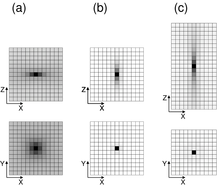
FIG. 1.: (a) Intersite correlations of AFD local modes $\langle a_{z}(0,0,0)a_{z}(x,y,z)\rangle$ in SrTiO₃ at $T$=150K. The correlations in the $x$-$z$ plane ($y=0$, top) and the $x$-$y$ plane ($z=0$, bottom) are shown. Each small square represents one lattice site; the origin lies at the center. Grey scale denotes the degree of correlation: black for perfect correlation, white for zero correlation. (b) Same for FE local-mode correlations $\langle f_{z}(0,0,0)f_{z}(x,y,z)\rangle$. (c) Corresponding FE local-mode correlations in BaTiO₃ at $T$=320K.

Thermodynamic properties for this compound have been calculated and published in Ref. [14]. A pressure $P_{0}=-5.4$GPa is applied to restore the experimental lattice constant. A transition from the cubic phase to a tetragonal AFD structure at 130K, and two further FE phase transitions at 70K and 10K, were predicted. A later quantum path-integral MC simulation revealed that quantum fluctuations suppress the FE phases entirely, and reduce the AFD phase transition temperature to 110K.[21] This gives excellent agreement with experiment, which reveals a single AFD phase transition at 105K,[22] and no unambiguous phase transition (but the presence of “quantum paraelectric” behavior [23, 24, 25]) at low temperature. Our calculated pressure-temperature phase diagram showed that the FE and AFD instabilities have opposite trends with pressure, and FE and AFD instabilities tend to suppress each other.

We have performed some further simulations to investigate the behavior of the AFD and FE local modes, and in particular the nature of the intersite correlations for FE and AFD local modes in the cubic phase but just above the phase transition temperature. The M-point AFD modes do not appear to be important for SrTiO₃, so we focus on the two vector order parameters ${\bf f}(\Gamma)$ and ${\bf a}({\rm R})$ associated with the zone-center FE modes and the zone-corner AFD modes. Since the order parameters are vectors, the correlation functions are second-rank tensors. These can be calculated from our simulations as

$$S_{\alpha\beta}(x,y,z)=\langle v_{\alpha}(x_{0},y_{0},z_{0})v_{\beta}(x_{0}+x,y_{0}+y,z_{0}+z)\rangle\;,$$ (38)

where the average is taken over all the sites $x_{0},y_{0},z_{0}$ in the MC simulation cell and over all MC sweeps $t$. Here the $v_{\alpha}$ denote the components of the FE or AFD order parameters [$f_{\alpha}$ for FE, $a_{\alpha}(-)^{l+m+n}$ for AFD, where ${\bf R}_{i}=l{\bf x}+m{\bf y}+n{\bf z}$]. We can get a good picture of the nature of the correlation by investigating the diagonal elements ($\alpha=\beta$) only. Since the three Cartesian directions are equivalent, it suffices to present $S_{zz}(x,y,z)$.

In Fig. 1(a), we show the calculated AFD correlation function $S^{\rm AFD}_{zz}(x,y,z)$ in the two planes $x$-$z$ and $x$-$y$ for SrTiO₃ at T=150K, in the cubic phase but just above the AFD phase transition temperature of 130K. We find that the correlations are quite strong in $x$-$y$ plane, with a correlation length of about three lattice constants. Along the $z$ direction, even the nearest-neighbor vectors are almost completely uncorrelated. Thus, the shape of the “equal correlation surface” for AFD local modes is disc-like. This is easy to understand on the basis of the RUM picture.[2] Since the AFD local modes involve a rotation of oxygen octahedra, and any distortion of the oxygen octahedra involves a large energy cost (as shown by the large magnitude of $j_{1}$, $j_{4}$, and $j_{8}$), the AFD octahedral rotations about $\hat{\bf z}$ correlate strongly in the $x$-$y$ direction. On the other hand, the rigidness of the octahedra does not impose any relation between $z$-polarized AFD modes in different $z$ planes (as reflected in the very small $j_{2}$). Thus, the pancake-like correlation naturally results.

Fig. 1(b) shows the corresponding FE correlation function $S^{\rm FE}_{zz}(x,y,z)$ for SrTiO₃ at T=150K (the FE phase transition occurs at 70K). Its behavior is just the reverse of the AFD modes, being strong along the $z$ direction and weak in the $x$-$y$ plane, and resulting in a needle-shaped “equal correlation surface.” This behavior is a direct consequence of the anomalously large mode effective charges in the cubic perovskite compounds[26] which strongly suppress the longitudinal FE fluctuations and leads to the strong correlation of $f_{z}$ in the $z$ direction. On the other hand, the transverse FE modes can easily go soft, resulting in a short correlation length for $f_{z}$ in the $x$-$y$ plane.

The above picture of the correlation functions for AFD and FE local modes are presumably quite general for the cubic perovskite compounds. For the FE modes, we decided to repeat the calculations for the case of BaTiO₃, where the AFD instability does not intervene. We show in Fig. 1(c) the correlation function calculated in the cubic phase at T=320K, about 20K above the FE phase transition temperature. We can see the behavior of the correlations is again needle-like and even more pronounced than for SrTiO₃, presumably because we are closer to the FE transition temperature. (An elongated supercell was used to accomodate the correlations in this case.)

FIG. 2.: The probability distribution of the Cartesian component of the local-mode variable $a_{x}$ for SrTiO₃ in the cubic phase at $T$=140K (dashed line) and $T$=150K (solid line).

As was done for the FE modes in BaTiO₃,[11] it is revealing to compute the equilibrium distribution of one cartesian component of the AFD order parameter ${\bf a}({\rm R})$ in the cubic phase just above the phase transition temperature in SrTiO₃. This is shown in Fig. 2, where it can be seen that the distribution looks approximately Maxwellian. This is indicative of a transition having a character much closer to the displacive than to the order-disorder limit.

B CaTiO₃

CaTiO₃ is one of the more complicated perovskites. Experimentally, it is found to have two stable phases, an orthorhombic phase at lower $T$ and a cubic phase above $1530$K.[27] Some recent experiments suggest that the transition is to a highly disordered cubic phase.[28] The room-temperature orthorhombic phase has a very complicated structure with a 20-atom unit cell. The displacements of all the atoms away from their idea positions have been determined in Ref. [29]. The refined structure as a function of temperature has also been determined recently using X-ray diffraction.[30, 31] This complicated structure can be decomposed into a simultaneous freezing in of three AFD modes: an R-point mode polarized along (1$\bar{1}$0) with rotation angle 0.20 (angles in radians), an M-point mode polarized along (001) with rotation angle 0.14, and an X-point mode polarized along (1$\bar{1}$0). The X-point mode involves not only the rotation of oxygen octahedra, but also an associated displacement of Ca atoms. The ratio of O and Ca displacement is about $1:-3$ and the oxygen octahedral rotation angle is only about 0.03.

For such a complicated structure, even a complete first-principles determination of its $T=0$ structure would be very difficult. However, we can arrive at a partial understanding of this structure as follows. Our calculations show that the reference cubic structure is unstable towards either the R-point or the M-point AFD mode individually (negative $\omega^{2}$), whereas it is stable with respect to the X-point mode individually (positive $\omega^{2}$, no double-well behavior). In fact, the X-point mode involves a strong distortion of the oxygen octahedron, and thus is far from soft. However, the symmetry of the crystal is such that if both the R-point and M-point AFD mode distortions are already simultaneously present, then the Ca and O atoms experience forces in the pattern of the X-point mode, as a result of the cubic anharmonic interactions discussed in Sec. IIB. Thus, under these conditions the crystal would necessarily acquire some X-point mode distortion. We therefor conclude that the appearance of the X-point mode distortion must be the result of the third-order coupling between R-, M-, and X-point AFD modes. This is a major reason why we chose to include the third-order coupling in our model Hamiltonian. The strain coupling is expected to be important in the determination of the actual magnitude of the X-mode distortion, complicating the problem and making a complete quantitative LDA determination of the X-mode amplitude difficult.

FIG. 3.: (a) Calculated AFD order parameters $a(R)$ of CaTiO₃ vs. $T$ at $P_{0}=-11.3$GPa. (b) Calculated FE and AFD order parameters of NaNbO₃ vs. $T$ at $P_{0}=-4.3$GPa.

To obtain the phase transition sequence, we start the MC simulation at a high temperature ($T>2000$K) and equilibrate the system for 10,000 MC sweeps. An isotropic pressure $P_{0}=-11.3$GPa is imposed to restore the experimental lattice constant, and all the subsequent simulations are done under this pressure. The temperature is reduced in small steps (as small as 10K around the transition temperature) with 30,000 MC sweeps at each $T$ to ensure equilibration. The order parameters are accumulated over the last 20,000 MC sweeps, after checking that they do not vary significantly over this period. In our simulation, we find that except for the R-point AFD order parameters ${\bf a}({\rm R})$, all other FE or AFD order parameters are zero throughout the simulation. So the only phase transition we observe is associated with ${\bf a}({\rm R})$. Fig. 1(a) shows the calculated order parameters ${\bf a}(R)$ as a function of temperature. (What we actually plot are the averaged maximum, intermediate, and minimum absolute values of the order-parameter components.) At high temperature ($T>1800$K) the system is in the cubic structure, where all the components are zero. The material goes through a phase transition at 1750K, where all three order parameter components increase simultaneously. Our phase transition temperature is close to the experimentally measured 1530K, but we obtain the wrong low-temperature structure. Ours is rhombohedral with a 10-atom cell, instead of orthorhombic with a 20-atom cell as observed experimentally.

The difference between our theoretical result and experiment is not quite as dramatic as it might seem. Both the structure and the structural energy are very similar for the R-point and the M-point AFD mode polarized along (001). Note that in the observed structure, the amplitude of the M-point mode is about $\sqrt{2}/2$ times the the amplitude of the R-point mode polarized in the (1$\bar{1}$0) direction. Thus, we can say that the main difference between our calculated structure and the observed one is that one component of the R-point AFD mode is replaced by an M-point mode in the observed structure. As argued above, the additional presence of the X mode is just a result of third-order anharmonic coupling. In fact, we find that if we artificially increase the third-order coupling constant $B_{3}$ by a factor of 5, we recover the experimental $T=0$ structure in our MC simulations.

Clearly, the fact that the structure is strongly affected by relatively weak anharmonic intersite interactions makes the determination of the correct low-temperature phase very difficult in CaTiO₃. It is possible that a more careful treatment of the cubic intersite interactions (for example, an independent determination of the coupling constants associated with all three of the cubic anharmonic invariants discussed in Sec. II.B, or three-site or further-neighbor terms) might bring a better agreement with experiment, although one should not rule out the possibility that neglect of quantum fluctuations[21] or intrinsic limitations of the LDA might be at fault.

C NaNbO₃

Experimentally, NaNbO₃ is probably the most complex cubic perovskite known. The high-temperature phase is the simple prototype cubic structure as in the other cubic perovskites. Below 910K, a whole series of structural phase transitions has been found and at least six more phases have been identified. As the temperature decreases, the compound first goes through a cubic–tetragonal transition at 910K with freezing in of ${\bf a}({\rm R})$ modes polarized along one axis. There are then three orthorhombic phases present in the temperature range 845–638K, the most complicated having a unit cell containing 24 NaNbO₃ formula units. All of these phases can be regarded as given by rigid rotations of oxygen octahedra, accompanied by small induced X-point distortions. From 638K down to at least 170K, NaNbO₃ is antiferroelectric with an orthorhombic unit cell containing eight formula units. At even lower temperature, the crystal has been reported to transform into either a rhombohedral [32] or monoclinic[1] structure.

The complexity of the structural phase-transition sequence suggests the presence of several competing structural instabilities with very similar free energies. In principle, all the distortions involved in the observed structures of NaNbO₃ are included in our model. However, it is not realistic to expect that the calculated structural energies and free energies will be in exactly the right order, given the complexity of the problem and the level of accuracy of current first-principles based approaches. Nevertheless, we believe a first-principles study of NaNbO₃ is still important in identifying the most prominent distortions, as well as for demonstrating the limitations of such approaches.

The determination of the structure is done using MC simulations on a cubic $12\times 12\times 12$ simulation supercell. An isotropic pressure $P_{0}=-4.3$GPa is imposed to restore the experimental lattice constant, and all the subsequent simulations are done under this pressure. We start the simulation at very high temperature and equilibrate. The temperature is reduced in small steps ranging from 10K to 50K depending on proximity to a phase transition. At each temperature step, at least 40,000 MC sweeps are used to ensure that equilibrium is reached. The order parameters are accumulated over the last 30,000 MC sweeps.

The calculated averages of order parameters ${\bf a}({\rm R})$ and ${\bf f}(\Gamma)$ are shown in Fig. 1(b) as a function of temperature. All other modes are found to be zero throughout the simulation. As was the case for CaTiO₃, the averaged maximum, intermediate, and minimum absolute-value components are plotted. At high temperature ($T>800$K), the system is in the cubic structure with all the order-parameter components close to zero. As $T$ decreases to about 700K, one AFD component increases rapidly and becomes significantly non-zero, and the structure transforms from cubic to tetragonal. With further decrease of temperature, a second component became non-zero, indicating the occurrence of an orthorhombic phase. Below 560K, a third AFD component grows and the structure becomes rhombohedral. At very low temperature (below 50K), the simulation also apparently shows a sequence of three ferroelectric transitions, and the compound ends up in a rhombohedral ferroelectric structure at very low temperature.

Our first cubic–tetragonal phase transition compares favorably with experiment; we obtain the correct structure and underestimate the transition temperature by only $\sim$20%. In the orthorhombic phase, however, the calculated structure is much simpler than the observed one. Only one orthorhombic phase seems to occur in our simulation. However, Fig. 1(b) shows signs of fluctuations occurring in the vicinity of this phase (these fluctuations persist even if the number of MC sweeps is increased significantly). This indicates that the orthorhombic phase is not very stable, and may involve a mixing of different phases. Moreover, the transitions do not appear very distinct in Fig. 1(b) as a result of finite-size broadening, so increasing the lattice size may help to resolve the different phases. However, the computational load increases rapidly with increasing lattice size, and it becomes impractical to carry out simulations at much larger size. Our inability to get the correct AFE phase at room temperature is probably the most significant failure of our approach. Our zero-temperature structure is ferroelectric, but since the FE phases occur only at such low temperatures, it is likely that quantum fluctuations would need to be included to determine the actual low-temperature structure.[21]

V Discussion and Conclusion

In this and previous studies, we perform a series of ab initio studies of the thermodynamic properties of perovskite compounds. Without introducing any adjustable parameters, we have calculated structural transition sequences, transition temperatures, phase diagrams, and other thermodynamic properties based on first-principles calculations. For compounds with simple phase transitions, like BaTiO₃ and SrTiO₃, our calculated thermodynamic properties agree very well with experiment observations. For more complicated compounds like CaTiO₃ and NaNbO₃, our results are less satisfying.

There are two major sources of errors, the inaccuracy of LDA calculations and the imperfection of our models. Our LDA calculations have been carefully performed to avoid possible errors, and convergence has been carefully tested. As for the intrinsic accuracy of LDA, our calculated structural parameters and energies are within a few percent of experimental values. Although this is the usual high accuracy observed generally for the LDA, it is unfortunately not enough for truly accurate determination of the thermodynamic properties of perovskites. For example, it is embarrassing that we are forced to choose between carrying out the calculations at the theoretical equilibrium lattice constant or the experimental lattice constant (negative fictitious pressure); this choice can affect phase transition temperature by $\sim$100%. We regard this as being the most important probable source of error in our calculations.

It is also possible to improve our model Hamiltonian. For example, our restricted assumption for the form of the third-order intersite interactions may be lifted, resulting in a significantly more complicated model Hamiltonian. Also, other higher-order terms can be included in the Hamiltonian. It would also be possible to include more degrees of freedom per cell, or include eigenvector information from more k-points of the Brillouin zone when defining the local-mode vectors, to treat other phonon excitations more accurately.[33] However, in view of the current accuracy of first-principles calculations, we are not sure that these modifications would dramatically improve our results.

Finally, we emphasize that all of the MC simulations reported here treat the atomic motion purely classically. As mentioned above, we have recently reported results of quantum path-integral MC simulations showing that quantum fluctuations of the atomic coordinates (i.e., zero-point motion) can shift transition temperatures by tens of degrees, and in some cases even eliminate delicate phases.[21] Certainly this remains an important avenue of investigation for CaTiO₃ and NaNbO₃, but we nevertheless think it unlikely that inclusion of quantum fluctuations would immediately resolve the discrepancies with the experimental phase diagrams for these compounds.

In conclusion, we have extended our previous first-principles theory for perovskite ferroelectric phase transitions to treat also antiferrodistortive transitions. We apply this approach to the three cubic perovskite compounds SrTiO₃, CaTiO₃, and NaNbO₃, and calculate their thermodynamic properties including phase transition sequences and transition temperatures. For SrTiO₃, our calculated results are in good agreement with experiment. For CaTiO₃ and NaNbO₃, our calculated structural transitions have the correct general trend and the transition temperatures are in rough agreement with experiment, but the calculated transition sequences are not correct in detail. We attribute this to the larger distortions and many multiple competing instabilities in these compounds. For SrTiO₃, we also analyzed the intersite correlations for both FE and AFD local modes, finding needle-like and pancake-like correlations respectively for FE and AFD modes as expected on physical grounds.

- [1] M. E. Lines and A. M. Glass, Principles and Applications of Ferroelectrics and Related Materials (Clarendon Press, Oxford, 1977).
- [2] M. T. Dove, A. P. Giddy, and V. Heine, Ferroelectrics 136, 33 (1992).
- [3] E. Pytte, Phys. Rev. B 5, 3758 (1972).
- [4] A. D. Bruce and R. A. Cowley, Structural Phase Transitions (Taylor & Francis, London, 1981).
- [5] E. Pytte and J. Feder, Phys. Rev. 187, 1077 (1969); J. Feder and E. Pytte, Phys. Rev. B 1, 4803 (1970).
- [6] H. Bilz, G. Benedek, and A. Bussmann-Holder, Phys. Rev. B 87, 4840 (1987) and references therein.
- [7] G. Gordon and Y. S. Kim, J. Chem. Phys. 56, 3122 (1972); L. L. Boyer et al., Phys. Rev. Lett. 54, 1940 (1985); P. J. Edwardson et al., Phys. Rev. B 39, 9738 (1989).
- [8] R. E. Cohen and H. Krakauer, Phys. Rev. B 42, 6416 (1990); R. E. Cohen and H. Krakauer, Ferroelectrics 136, 65 (1992); R. E. Cohen, Nature 358, 136 (1992).
- [9] D. J. Singh and L. L. Boyer, Ferroelectrics 136, 95 (1992).
- [10] R. D. King-Smith and D. Vanderbilt, Phys. Rev. B 49, 5828 (1994); Ferroelectrics 136, 85 (1992).
- [11] W. Zhong, D. Vanderbilt, and K. M. Rabe, Phys. Rev. Lett. 73, 1861 (1994).
- [12] W. Zhong, D. Vanderbilt, and K. M. Rabe, Phys. Rev. B 52 6301 (1995).
- [13] K.M. Rabe and U.V. Waghmare, J. Phys. Chem. Solids, in press.
- [14] W. Zhong and D. Vanderbilt, Phys. Rev. Lett. 74, 2587 (1995).
- [15] Note the change of notation between Ref. 12 and this paper. Variables and here correspond to and in Ref. 12, respectively.
- [16] D. Vanderbilt, Phys. Rev. B 41, 7892 (1990).
- [17] M.C. Payne, M.P. Teter, D.C. Allan, T.A. Arias, and J.D. Joannopoulos, Rev. Mod. Phys. 64 1045 (1992).
- [18] T.A. Arias, M.C. Payne and J.D. Joannopoulos, Phys. Rev. Lett. 69, 1077 (1992).
- [19] H.J. Monkhorst and J.D. Pack, Phys. Rev. B 13, 5188 (1976).
- [20] M. P. Allen and D. J. Tildesley, Computer Simulation of Liquids (Oxford, New York, 1990); K. Binder, ed. The Monte Carlo Method in Condensed Matter Physics (Springer-Verlag, Berlin, 1992).
- [21] W. Zhong and David Vanderbilt, Phys. Rev. B 53, 5047 (1996).
- [22] G. Shirane and Y. Yamada, Phys. Rev. 177, 858 (1969); W. Buyers and R. Cowley, Solid State Commun. 7, 181 (1969).
- [23] K.A.Müller and H. Burkard, Phys. Rev. B 19, 3593 (1979); K.A.Müller, W. Berlinger, and E. Tosatti, Z. Phys. B 84, 277 (1991).
- [24] R. Viana et al., Phys. Rev. B 50, 601 (1994).
- [25] R. Martoňák and E. Tosatti, Phys. Rev. B 49, 12596 (1994).
- [26] W. Zhong, R. D. King-Smith and D. Vanderbilt, Phys. Rev. Lett. 72, 3618 (1994).
- [27] A. Granicher and O. Jakits, Nuove Cimento Suppl. 9, 480 (1954).
- [28] T. Vogt and W.W. Schmahl, Europhys. Lett. 24, 281 (1993).
- [29] H. F. Kay and P. C. Bailey, Acta Crystallogr. 10, 437 (1957).
- [30] X. Liu and R. C. Liebermann, Phys. Chem. Minerals 20, 171 (1993).
- [31] S. Sasaki, C. T. Prewitt, and J. D. Bass, Acta Crystallogr. 43, 1668 (1987).
- [32] Landolt-Bornstein Numerical Data and Functional Relationships in Science and Technology, edited by T. Mitsui et al. (Springer-Verlag, Berlin, 1981), NS, Group III, Vol. 16; ibid., edited by E. Nakamura et al., NS, Group III, Vol. 28.
- [33] K.M. Rabe, Phys. Rev. B 52, 13236 (1995).