Comparison of rigidity and connectivity percolation in two dimensions

Abstract

Using a recently developed algorithm for generic rigidity of two-dimensional graphs, we analyze rigidity and connectivity percolation transitions in two dimensions on lattices of linear size up to $L=4096$. We compare three different universality classes: The generic rigidity class; the connectivity class and; the generic “braced square net”(GBSN). We analyze the spanning cluster density $P_{\infty}$, the backbone density $P_{B}$ and the density of dangling ends $P_{D}$. In the generic rigidity and connectivity cases, the load-carrying component of the spanning cluster, the backbone, is fractal at $p_{c}$, so that the backbone density behaves as $B\sim(p-p_{c})^{\beta^{\prime}}$ for $p>p_{c}$. We estimate $\beta^{\prime}_{gr}=0.25\pm 0.02$ for generic rigidity and $\beta^{\prime}_{c}=0.467\pm 0.007$ for the connectivity case. We find the correlation length exponents, $\nu_{gr}=1.16\pm 0.03$ for generic rigidity compared to the exact value for connectivity $\nu_{c}=4/3$. In contrast the GBSN undergoes a first-order rigidity transition, with the backbone density being extensive at $p_{c}$, and undergoing a jump discontinuity on reducing $p$ across the transition. We define a model which tunes continuously between the GBSN and GR classes and show that the GR class is typical.

I Introduction

Scalar Percolation is a simple model for disordered systems, and has received much attention in the last two decades [1, 2, 3]. This model describes the transmission of a scalar conserved quantity (for example electric charge, or fluid mass) across a randomly diluted system. However in the calculation of mechanical properties force ( i.e. a vector) must be transmitted across the system [4]. It was originally suggested[6] that the critical behavior of the elastic moduli of a percolating system should be equivalent to that of its conductivity, but this is only valid for the scalar limit of the Born model of elasticity[5], a model which is not rotationally invariant and in many cases inappropriate. Elastic percolation is not in general equivalent to scalar percolation. This was first made clear by the work of Feng and Sen[7], which showed that central-force elasticity percolation was in a different universality class than scalar percolation, and provided the starting point for a renewed interest in this problem.

It soon became clear that the elasticity problem can be divided in two categories[13], according to the kind of forces which hold the lattice together. If angular forces are important[8, 9, 10, 11, 12, 15], a singly-connected path across the lattice is enough to ensure rigidity, so any configuration of bonds which is connected is also rigid. In this case, the geometry of the elastic backbone is exactly the same as that of the scalar percolation problem [9, 11, 12, 15]. This is the case for bond-bending[8, 9] and beam[10, 15] models. Thus, the elasticity percolation problem with angular forces is now well understood and that understanding has borrowed much from the geometrically equivalent scalar percolation problem. It is the purpose of this paper to analyze the more challenging central-force rigidity percolation transition, stressing the similarities and differences between this problem and scalar percolation.

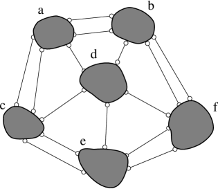
FIG. 1.: The six bodies shown in this figure are rigidly connected, i.e. they belong to the same rigid cluster. But the removal of any bond (thin black lines) leads to the collapse of the structure, which is then reduced to a collection of six independent rigid clusters (no two are rigidly connected). This means that the existence of a rigid connection between for example clusters $e$ and $f$ cannot be decided on local information only, since it depends on the presence of ’far away’ bonds, i.e. bonds not connected to clusters $e$ or $f$.

If rigidity [7, 14, 18, 20, 21, 22, 23, 25, 24, 32, 35] is provided by central forces alone (e.g. rotatable springs), single-connectedness is not enough to ensure rigidity. In this case a lattice that is conducting usually would not support an applied stress (i.e. it would not be rigid). This was first shown by Feng and Sen [7] who found that the rigidity threshold is significantly larger than the conductivity threshold. An exception worth mentioning is the case of elastic lattices under tension, or equivalently, systems in which all springs have zero repose length [16]. For such systems, conductivity and Young modulus are equivalent, i.e. rigidity appears at the scalar percolation point. It has been recently emphasized [17] that entropic effects can give rise to similar effects in central-force systems with nonzero repose length and finite temperature, although the connection with ref. [16] was not established.

The main difficulties associated with central-force elasticity are as follows: Whereas in the scalar connectivity case it is a trivial problem to determine when two sites belong to the same connected cluster, in the case of central-force rigidity it is not in general easy to decide whether two objects are rigidly connected. For example it takes some thinking to see that the six bodies in Fig. 1 form a rigid unit. Thus it is not easy to see how a computer algorithm can be devised to identify rigid clusters.

In the scalar connectivity problem, the removal of a singly-connected bond leads to the separation of a connected cluster into two clusters. In the rigidity case, the removal of an analogous “cutting bond” may produce the collapse of a rigid cluster to a collection of an arbitrarily large number of smaller ones (we call this the house-of-cards mechanism). Fig. 1 shows a simple example of this situation. Due to this fact, the transmission of rigidity can be “non-local” [14, 32], since a bond added between two clusters on one side of the sample may induce rigidity between two clusters on the other side of a sample.

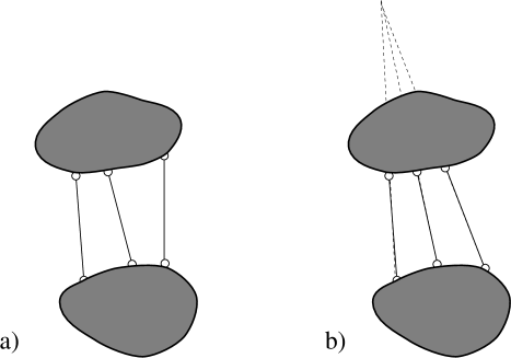
FIG. 2.: Three bars are in general enough to form a rigid connection between two rigid bodies (case a), but for particular, degenerate cases (case b), rigidity fails even when the system has the right number of bars. Case b fails to be rigid because the three bars happen to have a common point. A structure formed by two bodies connected by three bars is generically rigid in two dimensions if it is rigid “for most geometrical arrangements”, i.e. leaving aside degenerate configurations such as b), which occur with probability zero in the configuration space.

A second source of difficulties in the problem of central-force rigidity is the existence of particular geometrical arrangements for which a system may fail to be rigid [39] even if it is rigid for most other cases[28, 27, 30, 32]. Take for example two rigid bodies connected by three bars in two dimensions, as shown in Fig. 2. This structure is in general rigid, but if the three bars happen to have a common point, then the structure is not rigid, since this common point is the center of relative rotations[32] between the two bodies.

Particular geometrical arrangements (such as Fig. 2b), which are non-rigid even when the structure is rigid for most other configurations, are called degenerate configurations. Degenerate configurations appear with probability zero if the lattice locations are “randomly chosen”. A lattice is thus said to be generically rigid, if it is rigid for most geometrical arrangements of its sites. Generic rigidity only depends on the topology of the underlying graph, i.e. ignores the possibility of degeneracies. Since degenerate configurations are always possible on perfectly regular lattices, we will assume our lattice sites to have small random displacements, in which case generic rigidity applies.

Up to recently, no simple algorithms existed for the determination of the rigid-cluster structure of arbitrary lattices. Due to this, direct solving of the elastic equations was one of the few methods [4] available to obtain information on the structure of rigidly connected clusters. But this is very time-consuming and did not allow the study of large lattices. Previous simulations were for example not sufficiently precise to confirm or reject the proposal[18, 19, 20] that bond-bending and central-force elastic percolation might after all still be in the same universality class. This suggestion was not inconsistent with some numerical results obtained on small-sized systems[18, 19, 20, 21, 22].

Recently there has been a breakthrough in the system sizes accessible to numerical analysis[23, 24, 25], following the development of efficient graph-theoretic methods for the problem or generic rigidity in two dimensions[27, 30, 31]. Using such methods, we study the central-force rigidity percolation problem on randomly diluted triangular lattices of linear size up to $L=3200$, and connectivity percolation and body-joint rigidity percolation on site-diluted square lattices of size up to $L=4096$. Our numerical algorithm [30] is complementary to the “pebble game” [24, 31], which is an implementation of Hendrickson’s matching algorithm in the original “joint-bar” representation of the network [27](see below). This paper is an elaboration and extension of our two recent letters on this subject[23, 25]. We extend and elaborate upon the numerical data presented there in several ways: by comparing rigidity and connectivity percolation, by studying significantly larger lattices for rigidity percolation, by giving data on site and bond diluted lattices with a variety of boundary conditions; by presenting results on a new body-joint model which is in the universality class of bar-and-joint rigidity percolation and; by presenting detailed results for a model which continuously tunes between the braced square lattice (which has a first order rigidity transition) and the isotropic triangular lattice (which has a second order rigidity transition).

The numerical method is briefly described in Section II. In Section III, our results are presented and their implications discussed. A comparison is made with other available numerical and analytical results for the central-force rigidity percolation problem. We also discuss the issue of first-order rigidity, which has been the subject of a comment and reply in physical review letters[26]. Section IV contains our conclusions.

II The numerical method

We take an initially depleted triangular lattice and add bonds (in the bond-diluted case) or sites (in the site-diluted case) to it one at a time, and use a graph-theoretic matching algorithm [30] in order to identify the rigid clusters that are formed in the system. For the case of bond dilution, $p$ is the density of present bonds, while in site dilution it indicates the density of present sites. In the site-diluted problem, a bond is present if the two sites it connects are.

We use the body-bar version [30] of a recently proposed rigidity algorithm [27]. This algorithm, being combinatorial in nature, allows us to identify sets of sites which are rigidly connected, without providing any information on the actual values of the stresses when an external load is applied. The body-bar algorithm sees the lattice as a collection of rigid clusters (or “bodies”) connected by bars, instead of points connected by bars as proposed in the original algorithm[27] and as implemented in the “pebble game”[31]. The body-bar representation allows a more efficient use of CPU and memory, as each rigid cluster is represented as one object. The matching identifies rigid clusters and condenses them to one node as new bonds are added to the network.

In two-dimensional rigidity, a rigid cluster has $3$ degrees of freedom, while a point-like joint has $2$. Therefore the minimum number of bonds needed to rigidize $n$ joints in 2d is $(2n-3)$. Matching algorithms [27, 30, 31] are based on this sort of constraint-counting.

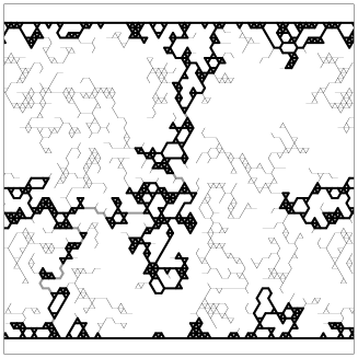
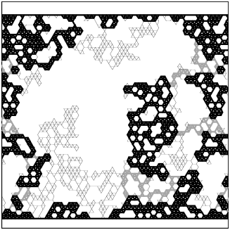
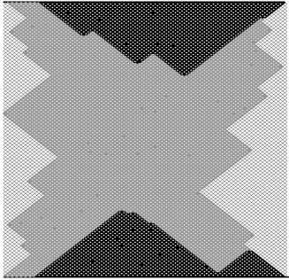
FIG. 3.: Infinite percolation clusters which lie in different universality classes: a) Connectivity percolation ($g=G=1$) on a triangular lattice; b) Rigidity percolation ($g=2,G=3$) on a triangular lattice; c) Rigidity percolation ($g=2,G=3$) on a braced square lattice. For a) and b), boundary conditions are periodic in the horizontal direction while for c) they are free. The system size $L=64$ and rigid bus-bars are set on the upper and lower ends of the sample. The backbone, is composed of ’blobs’ of internally stressed bonds (thick black lines), rigidly interconnected by cutting bonds (gray lines). Cutting bonds are also called red bonds. Removing one of them produces the collapse of the system. Dangling ends (thin lines) are rigidly connected to the backbone, but do not add to the ability of these networks to carry a DC external load (or current).

The body-bar algorithm [30], can be extended to handle “rigidity problems” with arbitrary values of $g$ (number of degrees of freedom of a joint) and $G$ (degrees of freedom of a rigid cluster). Connectivity for example, is just a special (simple) case of rigidity with $g=1$ and $G=1$: the minimum number of bonds needed to connect $n$ points is $n-1$ in any dimension. Connectivity percolation can thus be studied using this algorithm. More details on the application of matching algorithms for the specific case of connectivity percolation can be found in Ref. [43].

There are several ways to define the onset of global rigidity in a network [23]. We have used two distinct methods. First we determine whether an externally applied stress can be supported by the network, which we call applied stress (AS) percolation. Secondly we studied the percolation of internally-stressed (IS) regions.

At the AS percolation point, an applied stress is first able to be transmitted between the lower and upper sides of the sample. As we add bonds one at a time, we are able to exactly detect this percolation point by performing a simple test [30] which consists in connecting an additional fictitious spring between the upper and lower sides of the system. This auxiliary spring mimics the effect of an external load, and therefore the first time that a macroscopic rigid connection exists, a globally stressed region (the backbone) appears.

The IS critical point is defined as the bond- or site density at which internal stresses percolate through the system. This means that the upper and lower sides of the system belong to the same self-stressed cluster[23], and this is trivially detected within the matching algorithm[30]. The AS and IS definitions of percolation are in principle different, but we found [23] that the average percolation threshold and the critical indices coincide for large lattices. Similar definitions apply to the connectivity case, with the AS case being the usual definition, i.e. the onset of electric conductivity, and IS being percolation of “Eddy currents”.

We define the spanning cluster (Fig. 3) as the set of bonds that are rigidly connected to both sides of the sample. However only a subset of these bonds carry the applied load. This subset is called the backbone. The backbone will in general include some cutting bonds, so named because the removal of any one of them leads to the loss of global load carrying capability. Cutting bonds attain their maximum number exactly at $p_{c}$ [38]. The backbone bonds which are not cutting bonds are parts of internally overconstrained blobs. In the rigidity case, the smallest overconstrained cluster on a triangular lattice is the complete hexagonal wheel (twelve bonds), while in the connectivity case it is a triangle (i.e. the smallest possible loop). The spanning cluster also contains bonds which are rigidly connected to both ends of the sample but which do not carry any of the applied load. These are called dangling ends. This classification is standard in connectivity (scalar) percolation [37].

In this work we analyze several other boundary conditions, particularly in the generic rigidity case on triangular lattice. In that case, for site dilution we analyze: AS with rigid bus-bars at the ends of the sample, AS without bus bars (any-pair rigidity), and IS with bus-bars. For bond dilution, only the AS with bus-bars case was studied. We determine the exact percolation point (AS or IS) for each sample, so we can identify and measure the different components of the spanning cluster exactly at $p_{c}$ for each sample. This should be contrasted with usual numerical approaches, in which averages are done at fixed values of $p$, and $<p_{c}>$ is obtained from finite-size scaling (e.g. data collapse). In that case, it is known that slight differences in the estimation of $<p_{c}>$ can lead to important deviations in critical indices [18]. This source of error is absent in our measurements. Sample averages are done over approximately $10^{8}/L^{2}$ samples.

III Results

We first analyze the size dependence of the three key probabilities $P_{B}$, the backbone density, $P_{D}$, the dangling end density and $P_{\infty}$, the infinite cluster density, exactly at their percolation thresholds as described in the previous section. In Fig. 4a-c, this data is presented for the three different universality classes in Figs. 3a-c.

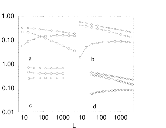
FIG. 4.: Density of backbone bonds (circles), dangling bonds (squares) and infinite cluster bonds (diamonds) at the AS critical point for: a) Connectivity percolation ($g=G=1$) on a site-diluted square lattice; b) Rigidity percolation ($g=2,G=3$) on a site-diluted triangular lattice; c) Rigidity on a randomly braced square lattice; d) Body rigidity ($G=g=3$) on a site-diluted square lattice .

Case c corresponds to the generic braced square net (GBSN), which is a square lattice to which diagonals are added at random with probability $p$. The non-generic version of this problem has been studied by many authors [33, 34, 35], and it is well known that the number of diagonals needed to rigidize it is not extensive: $p_{c}\sim 0$ when $L\to\infty$. This is confirmed by our numerical simulations, which correspond to the bus-bar boundary condition.

In Fig. 4d we also present data for the rigidity case $g=3,G=3$ on a square lattice, to further test whether the rigidity class is universal in two dimensions. In this model each site of a square lattice is a body and so has $g=3$ degrees of freedom. Each of these bodies is connected to each adjacent body by two bonds or bars, i.e. two contiguous bodies are pinned at a common point. Maxwell counting [46] then implies $f=3-4p$, so that the Maxwell estimate of the bond percolation threshold is $3/4$. Our numerical estimate is $p_{c}=0.74877\pm 0.00005$, thus confirming the accuracy of the Maxwell approximation.

One clear feature of Fig. 4 is that the BSN (Fig. 4c) has a qualitatively different behavior than the other cases. For the BSN, $P_{B}$, $P_{\infty}$ and $P_{D}$ all have a finite density at large $L$, indicating that the rigidity transition is first order in this case. In contrast, in both the connectivity(Fig. 4a) and rigidity cases (Figs. 4b,d), $P_{B}$ and $P_{\infty}$ are decreasing in a power law fashion over the available size ranges. However the behavior of $P_{D}$ is more complex. First we discuss the behavior of $P_{B}$.

At a second order phase transition, finite-size scaling theory predicts $P_{B}(p_{c})\sim L^{-\beta^{\prime}/\nu}$. Taking into account correction-to-scaling terms, which we assume to be power-law, we may generally write

$$P_{B}=C_{1}L^{-e}(1+C_{2}L^{-\omega}).$$ (1)

This expression is fitted to our numerical data by choosing the set of parameters $\{C_{1},C_{2},e,\omega\}$ that minimize the error

$$E=\sum\left(\frac{P_{B}^{measured}-P_{B}^{fit}}{P_{B}^{measured}}\right)^{2}.$$ (2)

A plot of $-log(P_{B})/log(L)$ vs. $1/log(L)$ should then have an asymptotic ($L\to\infty$) intercept equal to the leading exponent $e$. Similar fitting procedures were used to produce Figures 5 and 8, where the leading exponent is $\beta/\nu$ and $1/\nu$ respectively.

A fit of the data in Fig. 4b,d produces a rather universal estimate $\beta^{\prime}_{gr}/\nu=0.22\pm 0.02$. In consequence the rigid backbone is fractal at $p_{c}$, with a fractal dimension $D_{B}=1.78\pm 0.02$. In the connectivity case (Fig. 4a), we find [43] $\beta^{\prime}/\nu=0.350\pm 0.005$, or $D_{B}=1.650\pm 0.005$, which is consistent with the most precise prior work [44, 45].

Now we consider $P_{\infty}$ and $P_{D}$. In the connectivity case (Fig. 4a), an analysis of the dangling ends and infinite cluster probabilities (Fig. 5a) both lead to the estimate $\beta/\nu=0.10-0.11$, in agreement with the exact result 5/48. In the rigidity case however, there are strong finite size effects and even at sizes of $L=3200$ (joint-bar rigidity, Fig 4b), and $L=4096$ (body-joint rigidity, Fig. 4d, it looks as though the dangling probability may be saturating, while the infinite cluster density continues to decrease. Since $P_{\infty}=P_{B}+P_{D}$, it is expected that asymptotically $P_{\infty}$ and $P_{D}$ must behave in the same manner.

Clearly the numerical results for the range of system sizes currently available are still controlled by finite size effects, and the results depend on the analysis method chosen. Jacobs and Thorpe[24] chose to interpret the infinite cluster probability as being key. A fit to the $P_{\infty}$ data of Fig. 4b,d yields $\beta/\nu=0.147\pm 0.005$ (See Fig. 5b,c) in agreement with Jacobs and Thorpe. But a similar fit of the dangling end density gives $\beta/\nu\sim 0.03$ for the joint-bar rigidity case (Fig. 5b) and $\beta\sim 0.01$ for the body-joint rigidity case (Fig. 5c). In our previous work[25] we were guided by the Cayley tree results [36] which indicated a first order jump in the infinite cluster probability. We thus chose to interpret Fig. 4b,d as indicating a saturation of the infinite cluster probability at the dangling end value of about $0.1$. Having extended our data from $L=1024$ to $L=4096$, it now looks more likely that a small value of $\beta$ occurs in the rigidity case (Fig. 5b,c), though much larger simulation sizes are required to find $\beta/\nu$ precisely.

Due to the slow finite size effects found in the analysis of the infinite cluster and dangling end probabilities, it is natural to be concerned about the effect of boundary conditions and other, usually non-universal, parameters on the observed results. For generic joint-bar rigidity case on triangular lattices we thus tested a variety of different boundary conditions for both site and bond dilution. This data is presented in Fig. 6, from which it is seen that the conclusions drawn from the case of rigidity percolation with applied bus bars are quite robust.

FIG. 5.: The spanning cluster density exponent $\beta/\nu$ as numerically estimated for a) connectivity percolation on a square lattice ($L^{max}=4096$), b) rigidity percolation on a triangular lattice ($L^{max}=3200$) and c) body rigidity on a square lattice ($L^{max}=4096$). Two estimates result in each case from fitting the scaling of spanning cluster density (triangles) and dangling end density (circles). Solid lines are fits using Eq. (1)

Finally, the behavior of the dangling end density as a function of $p$ is also quite striking. This data is presented in Fig. 7. At very high $p$, nearly all bonds belong to the backbone, so the dangling end density approaches zero. Below $p_{c}$, there is no infinite cluster, so there are again no dangling ends. There then must be a maximum in the density of dangling ends between $p_{c}$ and $p=1$. As seen in Fig. 7, the interesting feature is the abrupt drop in the dangling density at $p_{c}$, a feature that appears to become more pronounced with increasing sample size. It is tempting to interpret this as definitive evidence of a first order rigidity transition, but it is also consistent with the strong finite size effects seen in Figs. 4b,d and Fig. 6, so we must await large lattice simulations for a definitive analysis.

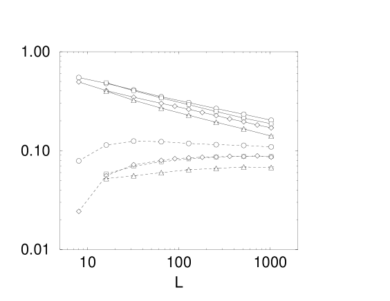
FIG. 6.: Backbone density $P_{B}$ (solid lines) and dangling-end density $P_{D}$ (dashed lines) as a function of sample size at the percolation threshold of each sample, on triangular lattices for: bond-diluted AS with bus-bars (circles), site-diluted AS with bus-bars (diamonds), site-diluted AS without bus-bars (triangles) and site-diluted IS without bus-bars. The AS percolation point without bus-bars is defined as the concentration of sites or bonds for which there is for the first time a rigid connection between at least one pair of points on opposite sides of the sample.

FIG. 7.: Fraction of dangling ends on the ($g=2,G=3$) generic rigidity infinite cluster, as a function of $p$, for site-diluted triangular lattices of size $L=$ 32, 64, 128, 256, 512 and 1024. Data shown here are for the AS case with bus-bars.

Now we turn to the calculation of the correlation length exponent for rigidity percolation. When there is a second-order rigidity transition, there is a diverging correlation length $\xi\sim|p-p_{c}|^{-\nu}$. We can find the exponent $\nu$ of this divergence by measuring the sample-to-sample fluctuations in $p_{c}$ as a function of $L$. The dispersion $\sigma(L)=\sqrt{(}<p_{c}^{2}>_{L}-<p_{c}>_{L}^{2})$, and according to finite-size-scaling $\sigma(L)\sim L^{-1/\nu}$.
FIG. 8.: The thermal exponent $1/\nu$ as numerically estimated for a) connectivity percolation ($g=G=1$) on square lattice, b) rigidity percolation ($g=2,G=3$) on a triangular lattice and c) body rigidity on a square lattice ($G=g=3$). Two independent estimates result in each case from fitting the scaling of red bonds (triangles) and fluctuations in $p_{c}$ (circles).

An asymptotic analysis for $\sigma(L)$ is shown in Fig. 8a for connectivity percolation, in 8b for joint-bar rigidity and in 8c for body-joint rigidity. From these figures we estimate $1/\nu=0.75\pm 0.01$ (the exact value is $1/\nu=3/4$) for connectivity percolation and $1/\nu=0.85\pm 0.02$ for rigidity percolation. This provides further strong evidence that rigidity percolation is second order in two dimensions, though not in the same universality class as scalar percolation. In the case of the first order rigidity on the braced square net (Fig. 9c), the variations in $p_{c}$ behave as $L^{-3/2}$, in accordance with analytical results for this model [40].

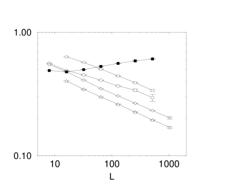
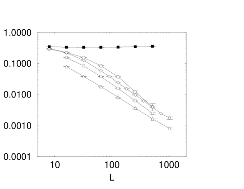
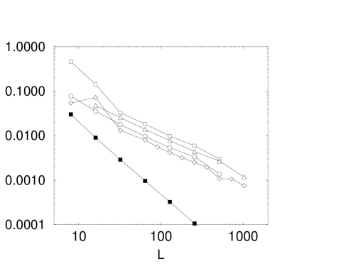
FIG. 9.: The volume fraction of a) backbone bonds b) cutting bonds, and c) the fluctuation $\sigma(p_{c})$ at the rigidity threshold for: Square lattice with $q=0$ - this is the braced square net (filled squares); Square lattice with $q=0.1$ (circles); Square lattice with $q=0.40$ (squares); Triangular lattice with bond dilution (diamonds) and Triangular lattice with site dilution (triangles).

Our algorithm also identifies the cutting (also called red or critical) bonds at the percolation point, for the case of AS percolation. The number $N_{R}$ of red bonds scales at $p_{c}$ as $L^{x}$. Coniglio [38] has shown that $x=1/\nu$ exactly, for scalar percolation. Numerical evidence suggesting that $x=1/\nu$ also in rigidity percolation was first presented in [23]. It is in fact possible to extend Coniglio’s reasoning to the case of central-force rigidity percolation [40]. It turns out that $x=1/\nu$ has to be rigorously satisfied also in this case, and therefore $\sigma(L)$ and $1/N_{R}(L)$ must have the same slope in a log-log plot. Analysis of the number of cutting bonds is also presented in Fig. 8, and yields values of $1/\nu$ consistent with the analysis of variations in percolation thresholds described in the previous paragraph.

Since the Cayley tree model [36] gives behavior quite similar to the braced square net [35], i.e. a first-order rigidity transition, it is interesting to ask whether the rigidity transition is “usually” like that on the braced square net (i.e. first order), or whether the second order transition found on triangular lattices is more typical. In order to probe this issue, we analyze a model which interpolates between the braced square net and the triangular lattice. In the braced square net, the random diagonals are present with probability $p_{d}$, to make the lattice rigid it is sufficient (though not necessary) to add one diagonal to every row of the square lattice. The probability that a spanning cluster exists is then $P_{+}=(1-(1-p_{d})^{L})^{L}$, from which we find $p_{d*}\sim lnL/L$.

We generalize this model by randomly adding the diagonals (with probability $p_{d}$) to a square lattice whose bonds have been diluted with probability $q$. The braced square net is $q=0$, while if $q=1-p_{d}$ this model is equivalent to the bond-diluted triangular lattice. Typical results for various values of $q$ are presented in Fig. 9. It is seen that even for a small amount of dilution of the square lattice, e.g. $q=0.10$, the rigidity transition returns to the behavior characteristic of the homogeneously diluted triangular case (see Fig. 9). We find that for sufficiently large lattice sizes, the universal behavior found in the other rigidity cases holds for any finite $q<0.5$ (for larger values of $q$ it is not possible to rigidize the lattice by randomly adding diagonals), and we suggest that the “fully-first-order” transition (i.e. a first-order backbone) only occurs in the special case of a perfect (undiluted) square lattice.

IV Conclusions

We have compared three types of percolation transition in two dimensions: the connectivity transition and; the generic rigidity transition on the triangular lattice and; the generic rigidity transition on the braced square lattice. A summary of our understanding is as follows: (i) The generic rigidity transition on triangular lattices is second order with $\nu=1.16\pm 0.03$, $0\leq\beta\leq 0.2$, $\beta^{\prime}=0.25\pm 0.02$ and; (ii) The rigidity transition on the braced square net is first order with finite backbone, spanning cluster and cutting bond densities at the percolation threshold. Only the value of $\beta$ for the generic rigidity transition on triangular lattices remains controversial, due to the very strong finite size effects in that case.

To illustrate the fact that our data is inconsistent with a first order backbone in the site-joint rigidity case, we have developed the following scaling argument.

Assume that the backbone mass[41] scales as $M_{B}\sim L^{D_{B}}$ at $p_{c}$. If the backbone is compact then $D_{B}=d$, the dimension of the system. The backbone mass is composed of red (or cutting) bonds plus “blobs” of overconstrained, or self-stressed bonds (See Fig. 3). Therefore $M_{B}=M_{red}+M_{blobs}$. The number of red bonds in the backbone scales as $M_{red}\sim L^{1/\nu}$, as analytical results [38, 40] and the simulations reported here show. Let us furthermore write $M_{blobs}=n_{blobs}\times m_{blobs}$ where $n_{blobs}$ is the number of blobs in the backbone, and $m_{blobs}$ be the average number of bonds in a blob. Therefore $L^{D_{B}}\sim L^{1/\nu}+n_{blobs}m_{blobs}$. Now, the AS backbone is an exactly isostatic body-bar structure, formed by rigid clusters (blobs) joined by bars (red bonds) so that counting of degrees of freedom is exact on it and so $M_{red}=3n_{blobs}+2n_{s}-3$ [30]. Here $n_{s}$ is the number of sites in the backbone, that do not belong to a blob (see Fig. 3). This identity is known as Laman’s condition[29, 30], and results from the fact that each red bond acts as a bar and therefore restricts one degree of freedom, while each blob has three degrees of freedom and isolated sites have two. The backbone is a rigid cluster and therefore has three overall degrees of freedom. We do not need to know $n_{s}$ for our argument. It is enough to notice that $n_{blobs}\leq M_{red}/3\sim L^{1/\nu}$. We can thus write

$$L^{D_{B}}\leq L^{1/\nu}(1+m_{blobs}/3)$$ (3)

To this point, we have made no assumption about the character (compact or fractal) of the backbone, so it is valid in general. If the transition is second-order, there is a divergent length (for example, the size of rigid clusters), and we expect $m_{blobs}$ to diverge with system size. Therefore a non-trivial value results for $D_{B}$, as we find numerically. If on the other hand there is no diverging length in the system, then $m_{blobs}\to$ constant for large systems and $D_{B}=d=1/\nu$ exactly. We thus see that a compact backbone requires an extensive number of cutting bonds, and this in turn can only be satisfied if $\nu=1/d$ exactly[42]. This is completely inconsistent with our data, and so the possibility of a first order backbone is remote in two dimensions.

The first order rigidity transition exhibited by the braced square net seems to be atypical as we illustrated using a model which tunes continuously from that limit toward the generic triangular lattice. We found that even a small deviation from the braced square lattice limit leads to a behavior similar to that of the triangular lattice. It would be intriguing if there were a tricritical point at which first order rigidity ceases and second order rigidity sets in, but we have not found a model which exhibits that behavior. Nevertheless there are a large number of other rigidity models in two dimensions, so the possibility is not yet ruled out.

C. M. acknowledges financial support of CNPq and FAPERJ, Brazil. This work has been partially supported by the DOE under contract DE-FG02-90ER45418, and the PRF. We are grateful to HLRZ Jülich for the continued use of their computational resources.

REFERENCES

- [1] D. Stauffer and A. Aharony, Introduction to Percolation Theory, 2nd. Edition (Taylor and Francis, London), 1994.
- [2] J. W. Essam, Percolation Theory, Rep. Prog. Phys. 43 (1980), 53.
- [3] A. Bunde and S. Havlin, Fractals and Disordered Systems, (Springer, Berlin), 1991.
- [4] M. Sahimi, Progress in Percolation Theory and its Applications, in: ”Annual Reviews of Computational Physics II”, edited by D. Stauffer, (World Scientific), 1995.
- [5] M. Born and K. Huang, Dynamical Theory of Crystal Lattices (Oxford Univ. Press, New York), 1954.
- [6] P. G. de Gennes,On a relation between percolation theory and the elasticity of gels, J. Physique Lett. (France) 37 (1976), L1.
- [7] S. Feng and P. Sen, Percolation on Elastic Networks: New Exponent and Threshold, Phys. Rev. Lett. 52 (1984), 216.
- [8] Y. Kantor and I. Webman, Elastic Properties of Random Percolating Systems, Phys. Rev. Lett. 52 (1984), 1891.
- [9] S. Feng, P. Sen, B. Halperin and C. Lobb, Percolation on two-dimensional elastic networks with rotationally invariant bond-bending forces, Phys. Rev. B 30 (1984), 5386.
- [10] S. Feng, Percolation properties of granular elastic networks in two dimensions, Phys. Rev. B 32 (1985), 510.
- [11] M. Sahimi, Relation between the critical exponent of elastic percolation networks and the conductivity and geometrical exponents, J. Phys. C: Solid State 19 (1986), L79-L83.
- [12] J. Zabolitsky, D. Bergmann and D. Stauffer, Precision Calculation of Elasticity for Percolation, J. Stat. Phys. 44 (1986), 211.
- [13] M. F. Thorpe, Rigidity Percolation, in “Physics of Disordered Materials”, edited by D. Adler, H. Fritzsche, and S. Ovishinsky (Plenum, New York), 1985.
- [14] A. Day, R. Tremblay and A.-M. Tremblay, Rigid Backbone: A New Geometry for Percolation, Phys. Rev. Lett. 56 (1986), 2501.
- [15] S. Roux, Relation between elastic and scalar transport exponent in percolation, J. Phys. A: Math. Gen. 19 (1986), L351.
- [16] W. Tang and M. F. Thorpe, Mapping between random central-force networks and random resistor networks, Phys. Rev. B 36 (1987), 3798; Percolation of elastic networks under tension, Phys. Rev. B 37 (1988), 5539.
- [17] M. Plischke and B. Joós, Phys. Rev. Lett. 80 (4907), 1998, B. Joós, M. Plischke, D.C. Vernon and Z. Zhou in Rigidity theory and applications, Edited by M.F. Thorpe and P.M. Duxbury (Plenum 1998).
- [18] S. Roux and A. Hansen, Transfer-Matrix Study of the Elastic Properties of Central-Force Percolation, Europhys. Lett. 6 (1988), 301.
- [19] A. Hansen and S. Roux, Multifractality in Elastic Percolation, J. Stat. Phys. 55 (1988), 759.
- [20] A. Hansen and S. Roux, Universality class of central-force percolation, Phys. Rev. B 40 (1989), 749.
- [21] M. Knackstedt and M. Sahimi, On the Universality of Geometrical and Transport Exponents of Rigidity Percolation. , J. Stat. Phys. 67 (1992), 887.
- [22] S. Arbabi and M. Sahimi, Mechanics of disordered solids. I. Percolation on elastic networks with central forces. , Phys. Rev. B 47 (1993), 695.
- [23] C. Moukarzel and P. M. Duxbury, Stressed backbone of random central-force systems, Phys. Rev. Lett. 75 (1995), 4055.
- [24] D. J. Jacobs and M. F. Thorpe, Generic Rigidity Percolation: The Pebble Game, Phys. Rev. Lett. 75 (1995), 4051. D. J. Jacobs and M. F. Thorpe, Generic rigidity percolation in two dimensions, Phys. Rev. E 53 (1996), 3683.
- [25] C. Moukarzel, P. M. Duxbury and P. Leath, Infinite cluster geometry in central-force networks, Phys. Rev. Lett. 78 (1997), 1480.
- [26] D. J. Jacobs and M. F. Thorpe, Phys. Rev. Lett. 80 (1998), 5451; P. M. Duxbury, C. Moukarzel and P. L. Leath, Phys. Rev. Lett. 80 (1998), 5452.
- [27] Bruce Hendrickson, Conditions for unique graph realization, SIAM J. Comput. 21(1992), 65.
- [28] H. Crapo Structural Rigidity, Structural Topology 1(1979), 26.
- [29] G. Laman, On Graphs and Rigidity of Plane Skeletal Structures, J. Eng. Math. 4, (1970), 331-340.
- [30] C. Moukarzel, An efficient algorithm for testing the rigidity of graphs in the plane, J. Phys. A: Math. Gen. 29 (1996), 8097.
- [31] D. Jacobs and B. Hendrickson, An algorithm for two-dimensional rigidity percolation: The pebble game, J. Comp. Phys. 137 (1997), 346.
- [32] E. Guyon et al., Non-local and non-linear problems in the mechanics of disordered systems: application to granular media and rigidity problems, Rep. Prog. Phys. 53 (1990), 373-419.
- [33] E. Bolker and H. Crapo, How to brace a one-story building, Environment and Planning B 4 (1977), 125; A. Recski, Applications of combinatoris to statics, Disc. Mathematics 108 (1992), 183; N. Chakravarty et. al., One-story buildings as tensegrity frameworks, Structural Topology 12 (1986), 11.
- [34] A. K. Dewney, The theory of rigidity, Scientific American, May issue 1991, p. 126
- [35] S. P. Obukov, First order rigidity transition in random rod networks, Phys. Rev. Lett. 74 (1995), 4472.
- [36] C. Moukarzel, P. M. Duxbury and P. L. Leath, First-order rigidity on Cayley Trees, Phys. Rev. E 55 (1997), 5800; P. M. Duxbury, D. Jacobs, M. F. Thorpe and C. Moukarzel, 1998 ppt. (cond-mat/9807073).
- [37] H. E. Stanley, Cluster shapes at the percolation threshold: an effective cluster dimension and its connection with critical exponents, J. Phys. A: Math. Gen. 10 (1977), L211; R. Pike and H. E. Stanley, J. Phys. A: Math. Gen. 14 (1981), L169.
- [38] A. Coniglio, Thermal phase transition of the dilute s-state Potts and n-vector models at the percolation threshold, Phys. Rev. Lett. 46 (1981), 250; Cluster structure near the percolation threshold, J. Phys. A: Math. Gen. 15 (1982), 3829.
- [39] We refer in this paper to “infinitesimal rigidity” as rigidity for short. Infinitesimal rigidity is a stronger condition than rigidity, and implies that no transformation, even an infinitesimal one, leaves all bar lengths invariant. See e.g. Refs. [28, 27, 30]
- [40] C. Moukarzel,(1996) unpublished.
- [41] We define the mass of the backbone as the number of bonds belonging to it. It is not correct to count sites in rigidity percolation, since they can simultaneously belong to several rigid clusters.
- [42] The randomly braced square lattice model has an extensive number of cutting bonds, but . Therefore it apparently violates Coniglio’s relation. The explanation is that only holds for the number of diagonals that are cutting bonds. There are, in addition to those, the cutting bonds which belong to the square lattice substrate, and these are . The reason for a completely first-order transition in this model is therefore the existence of an homogeneous, almost rigid substrate; the square lattice, which provides an extensive number of cutting bonds.
- [43] C. Moukarzel (1998), “A fast algorithm for backbones”, Int. J. Mod. Phys. C, to appear; (cond-mat/9801102).
- [44] M. Rintoul and H. Nakanishi, A precise determination of the backbone fractal dimension on two-dimensional percolation clusters, J. Phys. A: Math. Gen. 25 (1992), L945.
- [45] P. Grassberger, Spreading and backbone dimension of 2d percolation, J. Phys. A: Math. Gen. 25 (1992), 5475.
- [46] The Maxwell approximation consists in ignoring the existence of redundant bonds, i.e. assuming that each present bond eliminates one degree of freedom from a total of . The critical concentration is then obtained by equating to zero.