Longitudinal and transverse dissipation in a simple model for the vortex lattice with screening

Abstract

Transport properties of the vortex lattice in high temperature superconductors are studied using numerical simulations in the case in which the non-local interactions between vortex lines are dismissed. The results obtained for the longitudinal and transverse resistivities in the presence of quenched disorder are compared with the results of experimental measurements and other numerical simulations where the full interaction is considered. This work shows that the dependence on temperature of the resistivities is well described by the model without interactions, thus indicating that many of the transport characteristics of the vortex structure in real materials are mainly a consequence of the topological configuration of the vortex structure only. In addition, for highly anisotropic samples, a regime is obtained where longitudinal coherence is lost at temperatures where transverse coherence is still finite. I discuss the possibility of observing this regime in real samples.

]

I Introduction

Physical properties of the vortex structure in high temperature superconductors are strongly dependent on the values of some external parameters, such as magnetic field, anisotropy, and quenched disorder.[1] Some of these properties -as for example the existence of a first order melting transition in clean samples-[2] are originated in the interactions between vortices. Some others, however, are rather independent of the details of the interaction, and are related to the topological configuration of the vortex structure. It is interesting then to analyze in the simplest way the origin of those properties that depend only on the geometrical configuration of vortices, and not on their interaction. I concentrate in this paper on the behavior of the linear resistivity $\rho$ ($\rho=\lim_{I\rightarrow 0}V/I$) as a function of temperature -which has been widely used experimentally to unravel the properties of the vortex structure-,[1] both perpendicular and parallel to the applied magnetic field of a model that disregards non-local interactions between vortices. The results of numerical simulations on this model compare well with experimental results obtained in Y₁Ba₂Cu₃O₇ (YBCO, rather low anisotropy) and Bi₂Sr₂Ca₁Cu₂O₈ (BSCCO, high anisotropy) samples, as long as we consider zones of the phase diagram of the materials in which a first order transition is not observed. As stated above, the first order transition is generated by the interaction of vortices, and cannot be expected to occur in a model with only local interactions.

I describe the model in the next section, and the results in section III. The case of very high anisotropies deserves special attention and the limit of two-dimensional systems is discussed in section IV. The relevance of these results to real materials (in which vortices interact at finite -usually large- distances) is discussed in section V. Finally, in section VI, I summarize and conclude.

II Model

Vortices are modeled at different levels of detail when performing numerical simulations. A quite precise description is the Ginzburg-Landau theory, formulated in terms of the superconducting order parameter $\Psi\equiv\left|\Psi\right|\exp\left(i\theta\right)$.[3] In this context, when an external magnetic field or thermal fluctuations are introduced, vortices appear in the system as line-singularities around which $\oint\theta\left({\bf r}\right)d{\bf r}=2\pi$. A usual simplification which is appropriate in high temperature superconductors is to consider the modulus $\left|\Psi\right|$ of the order parameter as a constant, and keep only the phases $\theta\left({\bf r}\right)$ as the dynamic variables. This leads to the study of the uniformly frustrated $XY$ model,[4] which has been extensively studied, both because of its intrinsic properties and because of its applications to superconducting systems. As first shown by Villain,[5] the most important degrees of freedom of this model can be identified with the positions of the vortex in the system and an alternative description with these positions as the fundamental dynamical variables can be obtained. The original structure of the Ginzburg-Landau free energy is reflected at this level in the particular form of the interactions between vortices,[6, 7] which are cut off at distances of the order of the some penetration lengths $\lambda_{ab}$, $\lambda_{c}$ (the subindexes refer to the crystalline directions). These distances are in general large compared with the intervortex distance, and so the energy of the system has contributions coming from interaction between vortices that are far away from each other. I will consider here the case in which $\lambda$ is very small or, stated in another form, when the non-local terms of the interaction are dropped. In this case, the energy of a given configuration is simply proportional to the total length of vortices in the system. The investigation of the properties of the model in this case is important since, as we shall see, it gives insight on the behavior of the system with the full interaction, and allows to understand that the origin of many properties of the vortex lattice comes from the topological structure of vortex lines, and not from the exact nature of the interactions.

I will consider vortex segments lying on the bonds of a cubic mesh with periodic boundary conditions. Formally, the Hamiltonian of the system is

$$H_{0}=\sum_{i,\mu}{}^{\prime}\varepsilon_{i,\mu}\left(n_{i,\mu}\right)^{2},$$ (1)

where $n_{i,\mu}$ are integer variables defined on the nodes $i$ of the lattice, with direction $\mu$ ($\mu=$ a, b, c). The prime in the sum symbol indicates that only those configurations with zero divergence of the vector field $n$ have to be considered. The constants $\varepsilon_{i,\mu}$ are the energies of vortex segments at the positions $i,\mu$. We allow for the existence of anisotropy, defining a parameter $\eta$ as $\eta\equiv\left\langle\varepsilon_{i,c}\right\rangle/\left\langle\varepsilon_{i,ab}\right\rangle,$ with $\left\langle...\right\rangle$ indicating averaged values throughout the lattice. Disorder is introduced by allowing the values of $\varepsilon_{i,\mu}$ to be different in different points of the sample, fluctuating around the mean value. A disorder parameter (the same for the three spatial directions) is defined as $D=\left(\varepsilon_{i,\mu}^{\max}-\varepsilon_{i,\mu}^{\min}\right)/\left(\varepsilon_{i,\mu}^{\max}+\varepsilon_{i,\mu}^{\min}\right),$ with $\varepsilon_{i,\mu}^{\max}$ and $\varepsilon_{i,\mu}^{\min}$ being the maximum and minimum value of the energy of a vortex segment. The distribution between $\varepsilon_{i,\mu}^{\min}$ and $\varepsilon_{i,\mu}^{\max}$ is taken flat.

As the initial configuration of the system, a set of straight vortex lines directed along the c direction and uniformly distributed on the ab plane is considered. The number of vortices divided by the number of elementary plaquettes of the system perpendicular to the c direction defines the dimensionless magnetic field $H$. The Montecarlo process for updating the configuration consists in sequentially proposing the creation of elemental squared loops in all plaquettes of the lattice and with the three possible directions. The acceptance of the new configuration is carried out using a standard Metropolis algorithm. The initial configuration and the Montecarlo procedure guarantee that at any moment the vortex configuration has zero divergence. In order to calculate resistivities, both parallel and perpendicular to the applied field ($\rho_{c}$ and $\rho_{ab}$, respectively), we have to include a small external current $I$. This is done by adding a term to the Hamiltonian (1) that changes the energy of loops oriented perpendicularly to the current. One orientation increase its energy by $+I,$ and the other one decreases it in the same quantity. The value of the external current $I$ is chosen in such a way that the disbalance between right- and left-handed loops is never higher that 1/100 of the energy of the loop. In this regime of low currents the response is linear in the applied current, and resistivities do not depend on the exact value of $I$. The numerical results for different values of the anisotropy follow.

III Results for three dimensional samples

I will describe the results of the numerical simulations performed in systems with progressively higher anisotropies. Three different regions are distinguishable.

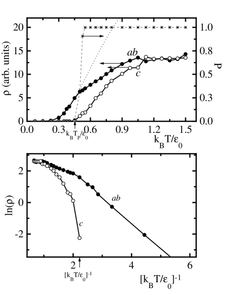
FIG. 1.: (a) Circles: resistivities along the ab and c directions using the Hamiltonian (1) for an isotropic lattice of size $40\times 40\times 8$ with $D=0$ and $H=1/4$. The dotted line is a fitting to a thermally activated movement of single vortices of the form $\rho_{ab}\sim\frac{1}{T}\exp\left(-2\varepsilon_{0}/k_{B}T\right)$. Stars: percolation probability as defined in text, note that this magnitude is (different from) zero only if $\rho_{c}$ is (different from) zero. (b) The resistivity values plotted to show thermally activated behaviors.

For low anisotropies, typical results for $\rho_{c}$ and $\rho_{ab}$ as a function of temperature are shown in Fig. 1 for a sample of size $L_{a}\times L_{b}\times L_{c}=40\times 40\times 8$ with $D=0$ (all $\varepsilon_{i,\mu}$ equal to $\varepsilon_{0}$) and $H=1/4$. As we see the ab dissipation has a thermally activated behavior (dotted line fitting) as long as the c axis dissipation is zero ($T<T_{P}$). The activation energy of this process is $2\varepsilon_{0},$ and corresponds to the energy necessary to create a double kink on a straight vortex, which is the first step in the process of movement. So in this region the dynamics of the system is that of a set of individual vortices thermally wandering into the sample. At a certain temperature $T_{P},$ the c axis dissipation $\rho_{c}$ becomes finite. The origin of this dissipation is related to a percolation transition of vortices occurring in the system, as studied before in the three dimensional Josephson junction array model.[8] For $T<T_{P}$ the vortices are practically independent, and a c axis directed current exerts no net force on them, thus generating no dissipation (in the linear regime). For $T>T_{P}$ the vortex lines are so heavily interconnected that vortex paths running (on average) in the ab direction appear. An external current applied along the c direction, being perpendicular to these paths, exert a net force on them and generates dissipation. In Fig. 1(a) we also see the value of the percolation probability $P$, defined as the fraction of time in which at least one percolation path is found in the system. It is clearly observed that the c axis dissipation is zero if $P$ is zero. The transition in the $P\left(T\right)$ curve between 0 and 1 becomes sharp in the limit $L_{ab}\rightarrow\infty$.[8]

An interesting effect of the percolation transition on the values of $\rho_{ab}$ is observed. When $\rho_{c}$ starts to be different from zero, the values of $\rho_{ab}$ deviate from the prediction of an activated behavior of individual vortices, and become smaller. This is an indication that for temperatures greater that $T_{P}$ the percolation of the vortex structure and the existence of many thermal excitations interferes with the thermally activated behavior of single vortices. In fact, for $T>T_{P}$ the concept of an isolated vortex in the system looses its sense, because we have a strongly entangled configuration of vortex lines. This effect of the percolation transition on the $\rho_{ab}\left(T\right)$ curve causes this to develop a typical shoulder that has been experimentally observed in measurements on YBCO samples,[9, 10] although its origin had not been clearly established.

In the case $D=0,$ when increasing anisotropy, the ab plane activation energy goes to zero as $1/\eta$ because this is mainly determined by the energy necessary to create a double kink, which is precisely $2/\eta$. Also the c axis transition is governed by an energy scale of the order of $\sim 1/\eta,$ because this temperature is mainly determined by the typical energy of the interlayer excitations (which goes as $\sim 1/\eta$). On heating, and from a practical point of view, the c axis transition occurs at a temperature at which $\rho_{ab}$ is clearly different from zero for all anisotropies.

The physics is richer in the case of samples with defects ($D\neq 0$). In this case, when anisotropy is increased, the activation energy for the ab dissipation tends to a value of the order of $D^{1/2},$ because the energy of a vortex segment piercing the ab plane is not constant in this case but has a dispersion of the order of $D^{1/2},$ and this is the typical energy barrier that has to be overcome when a vortex segment wanders within the ab planes. Anisotropy decreases the percolation temperature $T_{P}$ in a factor $\sim 1/\eta$, but has minor effect on the thermal activation in the planes as long as $D\neq 0$. Thus for high enough anisotropies, the c axis dissipation is expected to occur even at lower temperatures than the ab plane dissipation. However, when this range is approached a particular transition occurs in the system. The low temperature configuration of the vortex structure passes from a disentangled, and rather ordered configuration of vortex lines for low anisotropies, to an entangled configuration of vortex lines, i.e., we can say that the percolation temperature of the system drops abruptly to zero. The origin of this particular transition is the following. If anisotropy is low the system will prefer to remain ordered, with vortices almost straight in order to minimize their line energy. If anisotropy is increased, entangled configurations (in which vortices use the strongest pinning sites on the ab planes) diminish their energy and become locally stable, and from some value of the anisotropy, one entangled configuration becomes globally stable. This is the critical anisotropy $\eta_{1}$. This transition is related to the Bragg glass to vortex glass transition[11] proposed to occur in very anisotropic samples when increasing the magnetic field, because -as it has been discussed elsewhere-[12] an increase in the magnetic field is equivalent to an increase in the effective anisotropy and disorder of the system.

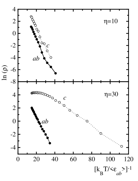
FIG. 2.: Typical results for $\rho_{c}$ and $\rho_{ab}$ as a function of temperature for two different values of anisotropy, in a sample of size $40\times 40\times 8$, with $D=0.5$ and $H=1/4$.

Numerical simulations indicate that in the $\eta>\eta_{1}$ regime both ab plane and c axis dissipation have a thermally activated behavior as shown in Fig. 2. The results for activation energies of $\rho_{c}$ and $\rho_{ab}$ as a function of anisotropy for a system of $40\times 40\times 8,$ with $D=0.5$ are shown in figure 3 (results for other values of $H$ are similar, with only a rescaling of the anisotropy axis). From a numerical (or experimental) point of view, it must be kept in mind that a thermally activated behavior with a given activation energy can be checked only for values of $k_{B}T$ greater than some fraction (which depends on sensibility) of the activation energy. In particular, no statements can be made about the possible existence of a true critical temperature much lower than that corresponding to the activation energy. In Fig. 3 and for $\eta<\eta_{1}\sim 4$ the c axis activation energy is not defined, because the transition is a percolation process and not a thermally activated process, as discussed before.

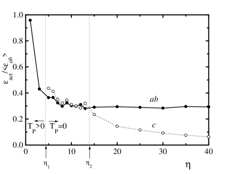
FIG. 3.: Activation energies for the dissipation along c and ab direction as a function of anisotropy (size $40\times 40\times 8$, $D=0.5$, $H=1/4$). For $\eta<\eta_{1}$ the c axis dissipation is not thermally activated but has a critical behavior instead. For $\eta>\eta_{2}$ the c axis activation energy decays as $1/\eta$.

The most direct and important conclusion from this figure is that there are two sub-regions in the range $\eta>\eta_{1}$. For $\eta_{1}<\eta<\eta_{2}$ activation energies for transport parallel and perpendicular to the field are rather similar, whereas for $\eta>\eta_{2}$ the c axis activation energy is lower than the corresponding to the ab plane. In the whole range $\eta>\eta_{1},$ ab plane activation energy is rather anisotropy independent, indicating that the ab plane dissipation is governed by the thermal activation of vertical segments of vortex lines pinned to the ab planes. For $\eta<\eta_{2}$ both parallel and perpendicular dissipation have the same activation energy indicating that they both originate in the same physical process.[13] In fact, ab plane dissipation is caused by the thermal depinning of vortex lines that cross the sample in the c direction. In turn, the c axis dissipation is caused by the thermal depinning of vortex lines that cross the sample in the ab direction (which exist because the vortex configuration is heavily entangled). However, as the formation of these paths is mediated by the externally generated vortices they are also pinned to the ab planes, and the activation energy for both processes is the same. Despite this, a global factor in the resistivity relation $\rho_{c}/\rho_{ab}$ depending upon the anisotropy and the geometrical configuration of vortex lines (especially on the relation between number of paths running along c axis and ab direction) is expected.

For $\eta>\eta_{2}$ the decrease of the activation energy for c axis dissipation as $1/\eta$ indicates that a new dissipation mechanism that depends only on the excitation of horizontal loops between planes is taking place. Being the vertical segments of vortex lines still frozen in the range of temperatures in which the c axis dissipation starts to be appreciable, this mechanism has to be related to processes occurring between consecutive ab planes, i.e., in the zone $\eta>\eta_{2}$ a complete decoupling of the planes takes place.

IV Perpendicular dissipation in two dimensional systems

As I mentioned in the previous section, the activation energy of the c axis dissipation at high anisotropies ($\eta>\eta_{2}$) goes to zero as $1/\eta,$ indicating that processes involving only the horizontal segments between consecutive planes are important. In order to understand clearly this kind of processes I will analyze the dissipation in the case of a unique horizontal plane.

Consider the model studied previously (Eq. 1) but now on a two dimensional geometry. It is useful to point out that this model (in the case without disorder) has been named in other context the roughening model of surfaces.[14, 15, 16] The mapping is made between vortex segments in the original model and height differences of a growing surface in the roughening model, the divergence free condition in the vortex model being the key property that makes possible the mapping. In the language of the roughening problem, the surface is smooth at large scales in the low temperature phase, and is rough in the high temperature phase. The long extending terraces that make the surface rough are no more than the infinite length vortex paths of the vortex model, and the growing rate of the surface maps onto the perpendicular resistivity of the vortex model. In the homogeneous case (without disorder), the roughening model is known to have an inverted Kosterlitz-Thouless transition at a temperature $T_{KT}\simeq$ $0.36\epsilon$ where $\epsilon$ is the energy of an elemental growing step (an elemental vortex loop in the vortex model, $\epsilon=4\varepsilon_{0}$).[17] This temperature can be viewed again as a percolation temperature of vortex lines in the vortex system: below the critical temperature $T_{KT}$ there is no infinite length paths, whereas for $T>T_{KT}$ these paths exist. In Fig. 4 the percolation probability for systems of different sizes is shown, and the transition is clearly distinguishable. As in the three dimensional case the transition in the variable $P\left(T\right)$ becomes sharp in the limit $L_{ab}\rightarrow\infty$. From known results on the roughening model[15] we can directly conclude that for an infinite system the perpendicular resistivity ($\rho_{c}$) jumps from zero to a finite value at the temperature $T_{KT}$.

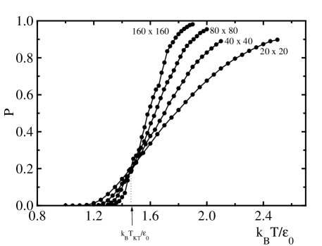
FIG. 4.: Percolation probability in a two-dimensional system without disorder for different system sizes. A phase transition in the limit of very large systems is clearly observed.

The disorder in the two-dimensional case may have two origins: one is the disorder introduced directly in the Hamiltonian, through the dependence of $\varepsilon_{i,\mu}$ on coordinates (Eq. (1)). The other comes from the existence in the 2D system of some quenched horizontal segments that come from the horizontal parts of the 3D vortices. This segments within the 2D system do not satisfy the condition $\nabla n=0,$ so its inclusion in the dynamics makes a non trivial contribution. We will concentrate on the second type of disorder for two reasons: numerical simulations show that the qualitative changes produced by the two types of disorder are similar, and secondly because this type of disorder is dynamical, and may change when changing anisotropy.

So the problem may be stated as that of a Hamiltonian

$$H=\sum_{i,\mu}{}^{\prime}\varepsilon_{0}\left(n_{i,\mu}-b_{i,\mu}\right)^{2},$$ (2)

where now $b_{i,\mu}$ represent the horizontal segments induced by the 3D vortices, and $\mu=a,b$. Note that the variables $n_{i,\mu}$ still satisfy the condition $\nabla n=0$, and the bare energy of the segments lying on the links has been taken to be $\varepsilon_{0}$ in all sites. It is interesting to consider the behavior of the system when the number of horizontal segments is being increased. We can characterize this value as the fraction of links in which $b_{i,\mu}=\pm 1,$ (which we denote by $D$). A necessary condition for a finite dissipation (perpendicular to the plane) is still that the vector field $n_{i,\mu}$ generates a path running all across the (two-dimensional) system. The probability of existence of such paths is shown for different sample sizes and different values of the disorder in Fig. 5(a). For $D<D_{cr}\simeq 0.3$ a well defined transition when the system size increases is detected. For finite disorder the transition temperature $T_{P}$ decreases with respect to the zero disorder value $T_{P}^{(D=0)}=T_{KT}\simeq 1.47$. If disorder is too high, however, there is no intersection of lines corresponding to different sizes, indicating that the percolation transition moves down to aero temperature. The behavior of the percolation temperature as a function of $D$ is plotted in Fig. 5(b).

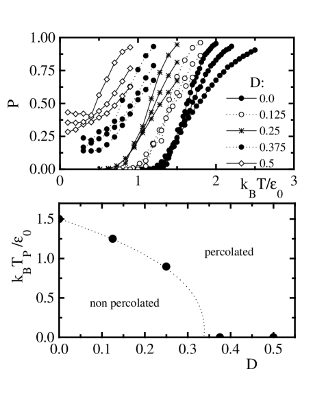
FIG. 5.: (a) Percolation probability in a two-dimensional system for different values of the disorder for system sizes $20\times 20$, $40\times 40$, and $80\times 80$ (from bottom to top, at the right of the curves). The results are the averaged values over 3 configurations of disorder for $D=0.125,$ $0.25,$ and over 8 configurations for $D=0.375,$ $0.5$. For $D<D_{cr}\simeq 0.3$ a percolation phase transition at finite temperature is clearly detectable. For higher values of disorder percolation temperature moves down to $T=0$. (b) Temperature of the percolation transition as a function of disorder as obtained from the results in panel (a). Points are the results of numerical simulations. Dotted line is a guide to the eye only.

Perpendicular resistivity simulations in this model (Fig. 6) give values that clearly go to zero in the case in which $T_{P}$ is finite ($D<0.3$)[18], and in the case when this variable is finite at any temperature give results that can be well fitted by a thermal activation expression. However, the possibility that the system has a real critical temperature at a temperature where the resistivity becomes undetectable in the simulations cannot be ruled out (see the note on the mapping to the roughening problem with disorder in the next paragraph).

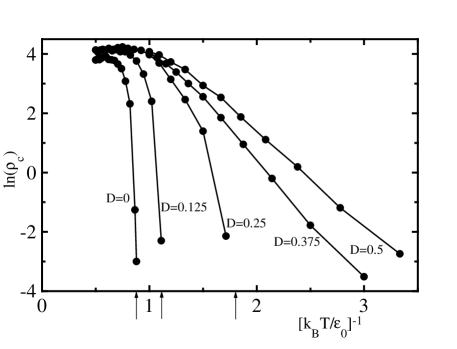
FIG. 6.: Perpendicular resistivity of a two dimensional system ($80\times 80$) as a function of temperature for different values of the concentration of quenched segments $D$. For $D<D_{cr}\simeq 0.3$ the approximate temperature at which temperature vanishes is indicated by arrows. For $D>D_{cr}$ the curves show activated low temperature tails.

The behavior of the percolation probability and resistivity for different values of $D$ of model (2) can be qualitatively explained using an argument of the type of the celebrated original Kosterlitz-Thouless argument for the phase transition in the two-dimensional $XY$ model. It goes as follows. The energy of a path running across a system of size $\sim L$ is the sum of $\sim L$ variables. According to (2), each of these variables may have the value $\varepsilon_{0}$, $-\varepsilon_{0}$, or $3\varepsilon_{0}$ depending if for that particular size the variable $b$ is $0,\pm 1$. The energy of the path becomes a Gaussian variable with mean value $\sim L$ and dispersion $\sqrt{LD\varepsilon_{0}}$. The total number of paths of length $\sim L$ running across the system is exponential in $L$, i.e., about $\sim e^{L}$. Taking into account these estimations, and considering the calculated number of paths with different energies as a density of states for non-interacting “particles”, it is possible to make the statistical mechanics of the system and look for the thermodynamic free energy of the equilibrium configuration. I only show the results, and not the details of the calculations, which are straightforward. Two clearly different regions appear (see Fig. 7): there is a zone (labelled I) of high disorder or high temperature in which some percolation paths have negative free energy, and so their existence is thermodynamically stable. In the other zone (labelled II) with low temperature and disorder, all percolation paths have positive free energy and thus the configuration without any path is the stable one. In zone II the system does not contain any percolation paths, and its resistivity is zero. When passing to zone I increasing the temperature, many percolation paths become immediately accessible at the transition, and perpendicular resistivity jumps to a finite value. In the case $D>D_{cr}$ there are available percolation paths down to zero temperature, and its likely that resistivity remains finite (with a thermally activated behavior) up to zero temperature, although a critical behavior of the resistivity at some finite temperature cannot be completely ruled out from these qualitative arguments.[19] These estimates compare well with the numerical results on Hamiltonian (2) (Figures (5) and (6)).

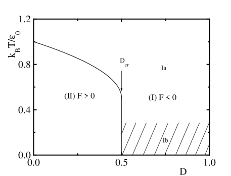
FIG. 7.: Qualitative phase diagram from the estimation of free energy of percolation paths, as discussed in the text. Zone I is a region with finite linear dissipation. Zone II has zero linear dissipation. The labels Ia and Ib and the dashed region are linked to the discussion presented in [18].

The mechanism discussed in this section for the perpendicular dissipation of a two-dimensional system is the responsible of the c axis dissipation in the three dimensional case for $\eta>\eta_{2}$ discussed in the previous section. As it was indicated before this mechanism relies on the movement of vortex segments between consecutive ab planes, contrary to the dissipation occurring for $\eta<\eta_{2}$ which involves paths that occupy a finite thickness along the c direction.

V Relevance to real materials. Effect of non local interactions

In spite of its simplicity, the previously studied model reproduces many characteristics of real transport measurements in high-$T_{c}$ superconductors, indicating that some of these properties are rather independent of the exact form of the interaction, and they are only consequences of geometrical properties. In particular, the case $\eta<\eta_{1}$ (Fig. 3) gives results which are comparable to experimental results in YBCO.[10, 20] In this case the c axis resistivity has been observed to appear only at higher temperatures than the ab dissipation, and a shoulder in $\rho_{ab}$ near $T_{P}$ similar to that of Fig.1 has been experimentally observed. Numerical simulations using the complete vortex-vortex interaction give also the same qualitative behavior.[21, 8] The results of the previous sections for the activation energy in the range $\eta_{1}<\eta<\eta_{2}$, namely the coincidence of activation energies for $\rho_{ab}$ and $\rho_{c},$ has been experimentally observed in BSCCO samples[22] and theoretically interpreted as an indication of the same origin for both dissipations in this regime.[13]

The only one region that gives a qualitatively new result is the range $\eta>\eta_{2}$, where a finite value for $\rho_{c}$ was obtained even at temperatures at which $\rho_{ab}$ is still negligible. We have to determine if this region can occur when the complete vortex-vortex interaction is taken into account or if it is a consequence of the local form of the interaction used in the model. The complete Hamiltonian for interacting vortex segments $n_{\mu}$ can be written in the generic form

$$H=\sum_{i,j}\sum_{\mu=a,b,c}G_{\mu}\left({\bf r}_{i}-{\bf r}_{j}\right)n_{\mu}\left({\bf r}_{i}\right)n_{\mu}\left({\bf r}_{j}\right).$$ (3)

where $G_{\mu}\left({\bf r}\right)$ is the non-local interaction function between segments (in previous sections I used this type of Hamiltonian with a local function $G$). The function $G_{ab}$ ($G_{c}$) is globally proportional to an energy scale that we can identify with our $\varepsilon_{ab}$ ($\varepsilon_{c}$) of equation (1), and the naive conclusion would be that in the highly anisotropic case ($\varepsilon_{ab}\ll\varepsilon_{c}$) the system of interplane vortices has a transition temperature $T_{1}$ of the order $k_{B}T_{1}$ $\simeq\varepsilon_{ab}$, whereas the system of vortex-antivortex pairs within the planes has a transition temperature $T_{2}$ of the order $k_{B}T_{2}$ $\simeq\varepsilon_{c}\gg k_{B}T_{1}$. However, the structure of the function $G$ for segments parallel to the layers

$$G_{ab}\left({\bf k}\right)=$$

$$=\frac{\varepsilon_{ab}}{\left[4-2\cos\left(k_{x}\right)-2\cos\left(k_{y}\right)\right]+\frac{\varepsilon_{ab}}{\varepsilon_{c}}\left[2-2\cos\left(k_{z}\right)\right]+\frac{\varepsilon_{ab}}{\Delta}}$$ (4)

(where $\sqrt{\Delta/\varepsilon_{ab}}\equiv\lambda_{c}$ is the magnetic penetration depth along the c direction in units of the lattice spacing) shows that the range of the interaction of parallel to plane segments increases with anisotropy as $\sim\left(\min\left[\varepsilon_{c},\Delta\right]/\varepsilon_{ab}\right)^{1/2},$ and this cannot be neglected.[7, 23] In fact, in the language of the renormalization group and in the case of very large $\lambda_{c}$, interacting horizontal segments renormalize to non-interacting segments but with an energy $\simeq\varepsilon_{ab}\left\{\left(\varepsilon_{c}/\varepsilon_{ab}\right)^{1/2}\right\}^{2}=\varepsilon_{c}$, so the transition temperature $T_{1}$ is of the order of $k_{B}T_{1}\simeq\varepsilon_{c}.$ A more detailed calculation[7] gives $T_{1}\sim 4\pi\min\left[\varepsilon_{c},2\Delta\right]$, $T_{2}\sim\frac{\pi}{2}\min\left[\varepsilon_{c},2\Delta\right].$ To have finite $\rho_{c}$ at temperatures where $\rho_{ab}$ is still zero is necessary at least that $T_{1}$ be lower than $T_{2},$ and this is not the case.

These estimates seem to rule out the practical possibility of a zone like that for $\eta>\eta_{2}$ in figure 3. However, the analysis made corresponds to the case of zero external field and disorder, and we know that the inclusion of them decreases the transition temperature of the interplane system of loops. So the question if in a finite external field, and for high anisotropies we can have a c axis transition temperature lower than the corresponding to the ab plane has still to be answered. The point cannot be fully discussed in all situations, but there is a limiting case in which it can be addressed. In fact, the case with a divergent anisotropy, in which the horizontal segments interact through a really long range potential, can surprisingly be discussed much easily that the case in which the interaction is local. Let us consider a finite value of $\varepsilon_{ab}$, and take $\varepsilon_{c},\Delta\rightarrow\infty,$ (so $T_{2}\rightarrow\infty$ also), and analyze the problem of the system of horizontal vortex segments between two consecutive planes. To be able to work with some indeterminations that will appear, the system size we will consider the system size will be considered finite with a value $L\times L$, and the limit $L\rightarrow\infty$ will be taken at the end. In this limiting case the function $G_{ab}\left({\bf k}\right)$ in terms of the two dimensional vector ${\bf k\equiv}\left(k_{x},k_{y}\right),$ reduces to $G_{ab}\left({\bf k}\right)=\varepsilon_{ab}/\left[4-2\cos\left(k_{x}\right)-2\cos\left(k_{y}\right)\right].$ Introducing (integer) loop variables $l({\bf r})$ through the substitution $\partial_{\mu}l\left({\bf r}\right)=n_{\mu}\left({\bf r}\right),$ and integrating by parts twice in the Hamiltonian, an equivalent model is obtained:

$$H=\varepsilon_{ab}\sum_{{\bf r}}\left(l\left({\bf r}\right)-\bar{l}\right)^{2}+I\sum_{{\bf r}}l\left({\bf r}\right),$$ (5)

where $\bar{l}=\sum_{{\bf r}}l\left({\bf r}\right)/L^{2},$ is the mean value of the loops variables over the $L^{2}$ plaquettes of the system. The time derivative of $\bar{l}$ is proportional to the voltage generated by the external current $I$. This expression is much easier to handle than the original formulation, and it is a sort of mean field Hamiltonian in which variables $l$ interact only through the $\bar{l}$ term. I stress however that no approximations other than the ones mentioned were done on passing from (3) to (5). When $L$ is large, the partition function corresponding to (5) can be calculated using a Lagrange multiplier for $\bar{l}$. The energy as a function of $\bar{l}$ becomes a periodic function of $\bar{l}$ (except by the current term), and in the limit $T\gg\varepsilon_{ab}$ it reads

$$E=L^{2}\left(-\frac{T^{2}}{\varepsilon_{ab}}e^{-\pi^{2}T/\varepsilon_{ab}}\cos\left(2\pi\bar{l}\right)+I\bar{l}\right).$$ (6)

When $L\rightarrow\infty,$ and for any value of temperature there is a critical value of $I,$ namely $I_{cr}=\frac{T^{2}}{\varepsilon_{ab}}e^{-\pi^{2}T/\varepsilon_{ab}}$. This critical current is nonzero for any temperature and thus indicates that the critical temperature of the system is infinite. This is consistent with the exact results since we took $\varepsilon_{c}\rightarrow\infty$. Notice, however, that the extremely small value of this critical current when $T$ is much larger that $\varepsilon_{ab}$ turns it difficult to verify this results in numerical simulations.

When quenched disorder due to horizontal segments of externally generated vortices are included, the previous picture changes in the following way. The potential due to these quenched segments is also long ranged, and on the $l$ variables they produce a potential that goes as $\sim\varepsilon_{ab}/r$. Summing up on each site the contributions from a random distribution of disorder on a sample of size $L$ gives a potential of typical amplitude $V\sim\varepsilon_{ab}D\left[\int^{L}\left(1/r\right)^{2}d^{2}r\right]^{1/2}\sim\varepsilon_{ab}D\sqrt{2\pi\ln L}$, where $D$ is the concentration of quenched segments. The Hamiltonian now reads

$$H^{D}=\varepsilon_{ab}\sum_{{\bf r}}\left(l\left({\bf r}\right)-\bar{l}\right)^{2}+I\sum_{{\bf r}}l\left({\bf r}\right)+$$

$$+\varepsilon_{ab}D\sqrt{2\pi\ln L}\sum_{{\bf r}}\chi_{{\bf r}}l\left({\bf r}\right).$$ (7)

The $\chi_{{\bf r}}$ are random variables with typical value $1$ and satisfying $\sum_{{\bf r}}\chi_{{\bf r}}=0$.[24] In the same way as before the energy of the system may be written in the form

$$E^{D}=L^{2}\left(-\frac{T^{2}}{\varepsilon_{ab}}e^{-\pi^{2}T/\varepsilon_{ab}}e^{-\pi^{3}D^{2}\ln L/2}\cos\left(2\pi\bar{l}\right)+I\bar{l}\right),$$ (8)

$$E^{D}=-\frac{T^{2}}{\varepsilon_{ab}}e^{-\pi^{2}T/\varepsilon_{ab}}L^{2-\pi^{3}D^{2}/2}\cos\left(2\pi\bar{l}\right)+L^{2}I\bar{l}.$$ (9)

When $L$ goes to infinity the first term will give an infinite activation energy -and thus a zero resistivity- if $D<2/\pi^{3/2}.$ On the other hand if $D>2/\pi^{3/2}$ activation energy goes to zero and the resistivity is finite. $D_{cr}=2/\pi^{3/2}$ is the critical value of the disorder in the system. As we see, in this case the c axis transition occurs at zero temperature, whereas the ab transition temperature is $\sim\varepsilon_{c}\rightarrow\infty$.

Thus at least in the case of infinite ranged interactions between vortex loops, it can be analytically shown that the c axis transition occurs at lower temperature than the ab transition, if disorder is greater than a critical value. This suggests that even in cases with finite $\varepsilon_{c}$, disorder can make longitudinal resistivity to appear at lower temperatures than transversal dissipation. The conclusion is that with the inclusion of the full interactions between vortices and for finite values of $\varepsilon_{ab}$ and $\varepsilon_{c}$ ($\varepsilon_{c}\gg\varepsilon_{ab}$), a phase diagram as the one sketched in Fig. 7 still holds, but with the zero disorder temperature transition being proportional to $\varepsilon_{c}$ rather to $\varepsilon_{ab}$. This indicates that a regime where $\rho_{c}\neq 0$ and $\rho_{ab}=0$ may be experimentally accessible in highly anisotropic and disordered samples.

VI Summary and conclusion

In this paper I have presented results from numerical simulations of vortex lattices in the presence of external magnetic field and quenched disorder, in which the interactions between vortices are neglected. In spite of the simplicity of the model the results reproduce qualitatively well many characteristics of the $\rho_{c}\left(T\right)$ and $\rho_{ab}\left(T\right)$ functions observed in experiments, both for YBCO samples, in which $\rho_{c}$ becomes different from zero when the value of $\rho_{ab}$ is already appreciable, and for BSCCO where experiments indicate that $\rho_{c}\left(T\right)$ and $\rho_{ab}\left(T\right)$ have thermally activated behaviors with the same activation energy. In addition, a new regime in which activation energy for $\rho_{c}\left(T\right)$ is lower than that for $\rho_{ab}\left(T\right)$ was found in the simulations, corresponding to the case where coherence length along c direction reduces to the distance between consecutive superconducting planes. Although in principle this regime may be an artifact of having disregarded interactions, I have shown it may occur in real samples in the presence of disorder, external magnetic field, and for high enough anisotropy.

VII Acknowledgments

I want to thank C. A. Balseiro and M. Goffman for discussions, and K. Hallberg for critical reading of the manuscript. This work was financially supported by Consejo Nacional de Investigaciones Científicas y Técnicas (CONICET), Argentina.

REFERENCES

- [1] For a review see G. Blatter et al., Rev. Mod. Phys. 66, 1125(1994).
- [2] W. K. Wkok et al., Phys. Rev. Lett. 69, 3370 (1992); H. Safar et al., Phys. Rev. Lett. 69, 824 (1992); H. Pastoriza et al., Phys. Rev. Lett. 72, 2951 (1994); E. Zeldov et al., Nature (London) 375, 373 (1995).
- [3] M. Tinkham, Introduction to Superconductivity (Krieger, Malaber, FL, 1980).
- [4] Y.-H. Li and S. Teitel, Phys. Rev. B 47, 359 (1993); C. Dasgupta and B. I. Halperin, Phys. Rev. Lett. 47, 1556 (1981); W. Y. Shih, C. Ebner, and D. Stroud, Phys. Rev. B 30, 134 (1984).
- [5] J. Villain, J. Phys. (Paris) 36, 591 (1975).
- [6] G. Carneiro, Phys. Rev. B 45, 2391 (1992); P. R. Thomas ans M. Stone, Nucl. Phys. B 144, 513 (1978).
- [7] S. E. Korshunov, Europhys. Lett. 11, 757 (1990).
- [8] E. A. Jagla and C. A. Balseiro, Phys. Rev. B 53, 538 (1996); ibid. 53, 15305 (1996).
- [9] K. W. Kwok et al., Phys. Rev. Lett. 69, 3370 (1992); S. Fleshler et al., Phys. Rev. B 47, 14448 (1993).
- [10] F. de la Cruz, D. López, and G. Nieva, Phylos. Mag. B 70, 773 (1994).
- [11] T. Giamarchi and P. Le Doussal, Phys. Rev. Lett. 72, 1530 (1994); Phys. Rev. B 52, 1242 (1995).
- [12] T. Chen and S. Teitel, preprint cond-mat#9610151; E. A. Jagla and C. A. Balseiro, Phys. Rev. B 55, 3192 (1997).
- [13] A. E. Koshelev, Phys. Rev. Lett. 76, 831 (1996).
- [14] S. T. Chui and J. D. Weeks, Phys. Rev. B 14, 4978 (1976); ibid. Phys. Rev. Lett. 40, 733 (1978).
- [15] D. Nozières anf F. Gallet, J. Phys. (Paris) 48, 853 (1987).
- [16] J. B. Kogut, Rev. Mod. Phys. 51, 659 (1979).
- [17] W. J. Shugard, J. D. Weeks, and G. H. Gilmer, Phys. Rev. Lett. 41, 1399 (1978).
- [18] Resistivity should vanish discontinuously at in systems of infinite size. This is not observed in Fig. 6 due to finite size effects.
- [19] It is interesting to compare these results with those that have been obtained for the roughening problem in the presence of disorder on the substrate. Although the way we are considering disorder in the two dimensional problem cannot be mapped exactly onto the disorder usually introduced in the roughening problem, (for the discussion of disorder on the roughening problem see J. Toner and D. P. Divincenzo, Phys. Rev. B 41, 632 (1990); J. L. Cardy and S. Ostlund, Phys. Rev. B 28, 6899 (1982)) it is noteworthy that a phase diagram qualitatively similar to that of Fig.7 has been obtained for this problem too (S. Scheidl, Phys. Rev. Lett. 75, 4760 (1995)). In this context, zone II is usually named the smooth phase, and zone I correspond to rough phases. However in this case a distinction within zone I is made between superrough (zone Ia, for lower that some “superroughening temperature” ) and rough (zone Ib, for ) phases. Diffusion of the surface (which maps onto perpendicular resistivity in our model) is zero in phases II and Ib, and is finite in zone Ia. The change of the diffusion coefficient is discontinuous when passing from zone II to Ib, and is continuous (critical) from zone Ia to Ib.
- [20] H. Safar et al., Phys. Rev. Lett. 72, 1272 (1994); D. López, G. Nieva, and F. de la Cruz, Phys. Rev. B 50, 7219 (1994).
- [21] E. A. Jagla and C. A. Balseiro, Phys. Rev. B 52, 4494 (1995).
- [22] R. Busch et al., Phys. Rev. Lett. 69, 522 (1992); Yu. I. Latyshev and A. F. Volkov, Physica (Amsterdam) 182C, 47 (1991); R. A. Doyle et al., Phys. Rev. Lett. 77, 1155 (1997).
- [23] This increase of correlation length with anisotropy implies that in numerical simulations much care must be taken when increasing the anisotropy . In fact, for a finite system size, if anisotropy is increased beyond , with the size of the sample and a numerical constant, the system behaves as a stack of single Josephson junctions, and of course c axis dissipation can be detected long before ab coherence is lost. This fact seems not to have been taking into account in some recent numerical simulations of highly anisotropic systems (A. K. Nguyen, A. Sudbø, and R. E. Hetzel, Phys. Rev. Lett. 77, 1592 (1996)).
- [24] The variables are spatially correlated, however this is unimportant because the interaction between s is only through the mean field variable .