Quantum critical exponents of a planar antiferromagnet

Abstract

We present high precision estimates of the exponents of a quantum phase transition in a planar antiferromagnet. This has been made possible by the recent development of cluster algorithms for quantum spin systems, the loop algorithms. Our results support the conjecture that the quantum Heisenberg antiferromagnet is in the same universality class as the O(3) nonlinear sigma model. The Berry phase in the Heisenbrg antiferromagnet do not seem to be relevant for the critical behavior.

I Introduction

Instead of classical transitions controlled by temperature $T$ a quantum phase transition between a symmetry broken phase with long-range Nèel order and a quantum disordered state with a finite spin excitation gap may be realized at $T=0$ by controlling a parameter $g$ to increase quantum fluctuations. Criticalities around such quantum phase transitions at $g=g_{c}$ may reflect inherent quantum dynamics of the system and yield unusual universality classes with rich physical phenomena.

The most prominent example are the high temperature superconductors. There the quantum spin fluctuations are thought to lead to $d$-wave superconductivity as soon as antiferromagnetism is suppressed by hole doping. This close connection between antiferromagnetism, quantum fluctuations and high temperature superconductivity has triggered many theoretical investigations.

Most of these investigations are based on a mapping to an effective field theory, the 2D O(3) quantum nonlinear sigma model. This sigma model is in the same universality class as the 3D O(3) classical sigma model or the 3D classical Heisenberg model. A large number of detailed predictions about quantum critical behavior has been made for the sigma model [1, 2]. However the spin-1/2 quantum antiferromagnet generally contains Berry phase terms [3] that are not present in the sigma model. The relevancy of these terms is not clear.

In order to shed light onto this question we have simulated a two dimensional quantum antiferromagnet (2D QAFM) that exhibits a quantum phase transitions. We calculate the critical exponents to determine the universality class and to check predictions made based on the nonlinear sigma model. First results have been published in Ref. [4].

A Quantum critical exponents

The critical exponents of a quantum phase transition at $T=0$ can be defined similar to a classical finite temperature phase transition. The quantum mechanical control parameter $g$ plays the role of the temperature in the classical system. Approaching the quantum critical point from the disordered side ($g>g_{c}$) the correlation length diverges as

$$\xi\propto(g-g_{c})^{-\nu}.$$ (1)

By the Trotter-Suzuki mapping the $d$-dimensional quantum system can be mapped onto a $d+1$-dimensional classical system. At zero temperature the system is infinite also in the additional imaginary time direction. The space and time dimensions are however not necessarily equivalent, and the correlation length in the time direction diverges in general with a different exponent

$$\xi_{\tau}\propto(g-g_{c})^{-z\nu},$$ (2)

where $z$ is the dynamical exponent. In a Lorentz invariant system space and time directions are equivalent and $z=1$. Related to the divergence of the correlation length is a vanishing of the spin excitation gap

$$\Delta\propto(g-g_{c})^{z\nu}.$$ (3)

When passing through the critical point long range order is established. The order parameter in the case of a Néel ordered antiferromagnet is the staggered magnetization

$$m_{s}=\left|{1\over N}\sum_{\bf r}e^{i{\bf Qr}}S^{z}_{\bf i}\right|^{2},$$ (4)

where $N$ is the number of spins in the lattice, $S^{z}_{\bf r}$ the $z$-component of the spin at site $\bf r$ and ${\bf Q}=(\pi,\pi)$. Close to the critical point the staggered magnetization behaves as

$$m_{s}\propto(g_{c}-g)^{\beta}.$$ (5)

At the critical point itself the real space correlation show a power-law falloff

$$\langle S^{z}_{\bf 0}S^{z}_{\bf r}\rangle\propto e^{i{\bf Qr}}r^{-(d+z-2+\eta)},$$ (6)

where $\eta$ is the correlation exponent. These three exponents are related by the usual scaling law

$$2\beta=(d+z-2+\eta)\nu,$$ (7)

where the effective dimension is $d+z$ in a quantum system.

B Predictions from the nonlinear sigma model

As mentioned above most analytic calculations of quantum critical behavior are based on the 2D O(3) quantum nonlinear sigma model (QNL$\sigma$M). Here we want to review the critical properties of the sigma model relevant for the current study.

TABLE I.: Critical exponents $\beta$, $\nu$, and $\eta$. Listed are both the estimates without making any assumption for $z$, and the best estimate if Lorentz invariance ($z=1$) is assumed. For comparison the exponents of the 3D classical Heisenberg (O(3)) model, the 3D Ising model and the 2D quantum mean field exponents are listed.

model	$\nu$	$\beta$	$\eta$
2D QAFM	$0.685\pm 0.035$	$0.345\pm 0.025$	$0.015\pm 0.020$
Lorentz invariant 2D QAFM	$0.695\pm 0.030$	$0.345\pm 0.025$	$0.033\pm 0.005$
3D O(3) [5]	$0.7048\pm 0.0030$	$0.3639\pm 0.0035$	$0.034\pm 0.005$
3D Ising [6]	$0.6294\pm 0.0002$	$0.326\pm 0.004$	$0.0327\pm 0.003$
mean field	1	1/2	0

The critical exponents of the QNL$\sigma$M can be determined from simple symmetry, universality and scaling arguments [1, 2]. Lorentz invariance implies that $z=1$. Furthermore the 2D QNL$\sigma$M is equivalent to the 3D classical sigma model. This in turn is in the universality class of the 3D classical O(3) model, or the classical 3D Heisenberg ferromagnet. The exponents $\beta$, $\nu$ and $\eta$ should thus be the same as the well known classical exponents of these models (see Tab. I).

Chakravarty, Halperin and Nelson have discussed the phase diagram of a planar Heisenberg antiferromagnet in the framework of the QNL$\sigma$M. They concentrate on the ordered phase and describe it as a classical 2D antiferromagnet with renormalized parameters.

TABLE II.: Universal prefactor $\Omega_{1}(\infty)$ in the linear temperature dependence of the uniform susceptibility at criticality. Listed are the results for the quantum nonlinear sigma model in a $1/N$ expansion, the results by classical Monte Carlo simulation on a 3D classical rotor model and the result of the present study.

method	Ref.	$\Omega_{1}(\infty)$
1/N expansion	[2]	0.2718
classical Monte Carlo	[2]	$0.25\pm 0.04$
quantum Monte Carlo	this study	$0.26\pm 0.01$

Chubukov, Sachdev and Ye have investigated the quantum critical regime of the QNL$\sigma$M in close detail [2]. They make some further predictions based on scaling arguments. On the ordered side the spin stiffness $\rho_{s}$ vanishes as

$$\rho_{s}\propto(g_{c}-g)^{(d+z-2)\nu}=(g_{c}-g)^{\nu},$$ (8)

where the second equivalence comes from the prediction that $z=1$. Additionally it follows from general scaling arguments that the uniform susceptibility at the critical point is universal:

$$\chi_{u}=\Omega_{1}(\infty)\left({g\mu_{B}\over\hbar c}\right)^{2}T.$$ (9)

Here $c$ is the spin wave velocity and $\Omega_{1}(\infty)$ a universal constant. Estimates for $\Omega_{1}(\infty)$ are listed in Tab. II.

The spin wave velocity $c$ scales as

$$c\propto(g_{c}-g)^{\nu(z-1)}$$ (10)

and is thus regular at the critical point if $z=1$.

C What about Berry phases?

The equivalence of the 2D QAFM to the 2D QNL$\sigma$M however is still an open question because of the existence of Berry phase terms in the QAFM that are not present in the QNL$\sigma$M [3]. It has been argued that these terms cancel in special cases, such as in the bilayer model [7, 8]. Then it is plausible that the quantum phase transition is in the same universality class as the QNL$\sigma$M. This was confirmed by quantum Monte Carlo calculations of Sandvik and coworkers [7, 9, 10]. They have investigated the finite size scaling of the ground state structure factor and susceptibilities on lattices with up to $10\times 10\times 2$ spins. Although these lattices are quite small they still found good agreement of the exponents $z$ and $\eta$ with the QNL$\sigma$M predictions [7, 9].

In another study Sandvik et al. [10] have investigated finite temperature properties of the bilayer QAFM on larger lattices and also found good agreement with the QNL$\sigma$M predictions. In the absence of Berry phase terms the equivalence of the QAFM and the QNL$\sigma$M is quite well established by these simulations.

But in general these Berry phase terms exist. Chakravarty et al. argue that they can change the critical behavior and lead to different exponents [1, 11]. Chubukov et al. on the other hand argue that the Berry phase terms are dangerously irrelevant [2] and do not influence the critical behavior.

Previous numerical simulations on dimerized square lattices [9, 12] are indeed not consistent with the QNL$\sigma$M predictions. Sandvik and Vekić [9] find a dynamical exponent $z\neq 1$, but their largest system was only $10\times 10$ spins. The deviation could be a problem with scaling arising from inequivalent spatial directions.

Katoh and Imada however found $z\approx 1$, compatible with Lorentz invariance. Additionally they calculated the correlation length $\xi$ and from it the exponent $\nu$. The validity of their result $\nu\approx 1$ is however again questionable because because of the restriction to very small lattices of $12\times 12$. On the other hand the discrepancy could be an effect of the Berry phase terms that are present in the dimerized square lattice but probably not in the bilayer.

The main purpose of the simulations reported is to she light onto this question and to clarify the role of the berry phase terms. Our results support the ideas of Chubukov et. al. [2] that the Berry phase terms are dangerously irrelevant.

II Algorithm and parallelization

Using the new quantum cluster algorithms, the loop algorithms [13, 14] it is possible to simulate much larger lattices at lower temperatures, just as the corresponding classical cluster algorithms have allowed the simulation of critical classical spin systems. With these algorithms it has for the first time become possible to study quantum critical spin systems in detail.

A disadvantage of the cluster methods however is that they cannot be vectorized as easily as the local update algorithms. Using powerful vector machines is therefore not an option. Fortunately however most of the modern supercomputers are parallel machines, and Monte Carlo methods are nearly ideally suited for that architecture.

One of the authors has developed an object oriented Monte Carlo library in C++ [15]. Using this library it is very simple to parallelize a Monte Carlo program and to port it to new parallel computers. The library automatically parallelizes any Monte Carlo simulation at the two “embarrassingly parallel” levels. The first level of trivial parallelism is the parameter parallelism. Simulation with different parameters, such as system size, coupling or temperature can be performed independently in parallel. At this level there is practically no overhead due to the parallelization. We get perfect speedup and the library takes care of load balancing.

A single simulation can similarly be parallelized by running it in parallel with different initial states and random seeds on each of the processors. The simulations run nearly independent. Communication is required only at the start and the end of the simulation. This level of parallelization incurs some overhead however. The overhead is the time used to thermalize a simulation. We loose efficiency if this thermalization time becomes comparable to the time actually needed for the simulation.

The third and deepest level of parallelization cannot be automatically done by the library since it depends on the algorithm used for Monte Carlo. The lattice used for one simulation can be spread over many processors. This parallelization has to be done by the programmer of the algorithm, but it is supported by various functions of the library. It is worthwhile to invest time in this parallelization only in two cases. The first is when, as mentioned above, thermalization is slow. Often the main reason is however different one. Large lattices simply might not fit into the memory of one processor.

In our simulations reported here we have used the 1024-node, 300 GFlop Hitachi SR2201 massively parallel computer of the university of Tokyo. At the time of its introduction this machine was the fastest general purpose computer in the world. Each processor has 256 MByte of local memory, enough to simulate quantum spin systems with 20000 spins at temperatures as low as $T=0.01$. This was large enough for the present study and we did not spend time on the third level of parallelization but used only the first two levels provided by the library.

The algorithm used was the continuous time loop algorithm [14]. The loop algorithms, first developed by Evertz et al. [13] are quantum version of the classical cluster algorithms. The continuous time version is preferable over the earlier discrete time versions since it eliminates the need to extrapolate in the finite Trotter time step $\Delta\tau$. In our experience we found that this leads to a four-fold speed increase. Additionally the continuous time algorithm uses only 10% of the memory compared to the discrete time algorithm, allowing the simulation of larger lattices.

III The CaV₄O₉ lattice

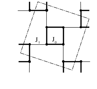
FIG. 1.: Lattice structure of the 1/5-th depleted square lattice of CaV₄O₉. The dashed square indicates the eight spin unit cell used in our calculations.

As the universality class of a phase transition does not depend on the microscopic details of the lattice structure we are free to choose the best lattice for our purposes. We have chosen the ${\rm CaV}_{4}{\rm O}_{9}$ lattice, a 1/5-th depleted square lattice depicted in Fig. 1 for our calculations. There are three reasons for this choice. Firstly the Berry phase terms are present on this lattice [16]. Next both space directions are equivalent, in contrast to the dimerized square lattice [9, 12]. This makes the scaling analysis easier. Finally at the quantum critical point all the couplings are nearly equal in magnitude, which is also optimal from a numerical point of view. We have performed our simulations on square lattices with $N=8n^{2}$ spins, where $n$ is an integer. Our largest lattices contained 20 000 spins. For the following discussion it is useful to introduce the linear system size $L$ in units of the bond lengths $a$ of the original square lattice: $L\equiv\sqrt{5N/4}a$.

FIG. 2.: Phase diagram of the CaV₄O₉ spin lattice as a function of the ratio $J_{0}/J_{1}$, reprinted from Ref. [17]. The leftmost point corresponds to the dimer limit $J_{0}=0$ and the rightmost point to the plaquette limit $J_{1}=0$. Circles indicate quantum Monte Carlo results for the spin gap, normalized by $J_{0}+J_{1}$. Diamonds show the staggered magnetization. As reference the perturbation theory estimates for the gap[18] and the linear spin wave theory (LSW) estimates for the staggered moment have been included.

The phase diagram of this lattice has been discussed in detail in Ref. [17] and is shown in Fig. 2. By removing every fifth spin we obtain a lattice consisting of four-spin plaquettes linked by dimer bonds. We label the couplings in a plaquette $J_{0}$ and the inter-plaquette couplings $J_{1}$. By controlling the ratio of these couplings $J_{1}/J_{0}$ we can tune from Néel order at $J_{1}=J_{0}$ to a quantum disordered “plaquette RVB” ground state with a spin gap $\Delta=J_{0}$ at $J_{1}=0$.

IV Results

A The critical point

The first step in the determination of the critical behavior is a high precision estimate of the critical coupling ratio $J_{1}/J_{0}$. We have calculated the second moment correlation length $\xi_{L}$ on systems of various sizes $L$. This can be determined in the usual way from the magnetic structure factor $S({\bf q})$ close to the Néel peak at ${\bf Q}$:

$$S({\bf Q}+\delta{\bf q})={S({\bf Q})\over 1+(||\delta{\bf q}||\xi)^{2}}+{\rm O}(\delta{\bf q}^{4}).$$ (11)

FIG. 3.: Plot of the ratio of correlation length divided by system size $\xi_{L}/L$. At the critical point the correlation length calculated in a finite system is proportional to the system size. This is the case for $(J_{1}/J_{0})_{c}=0.939\pm 0.001$.

The temperature was chosen to be $T=J_{0}/L$, keeping the finite $2+1$ dimensional system in the cubic regime. From standard finite size scaling arguments it follows that this correlation length $\xi_{L}$ scales proportional to the system size $L$ at criticality. We have calculated the ratio $\xi_{L}/L$ (shown in Fig. 3) for a variety of couplings and system sizes up to $N=9600$. Independence of the system size was seen at the critical coupling ratio $(J_{1}/J_{0})_{c}=0.939\pm 0.001$.

FIG. 4.: Finite size scaling of the staggered structure factor and susceptibility at the critical point.

B The exponents

Next we have calculated the finite size scaling of both the staggered structure factor $S({\bf Q})=L^{2}m_{s}$ and of the corresponding staggered susceptibility. At criticality they scale like

$$S({\bf Q}) \propto L^{2-z-\eta}$$ (12)

$$\chi_{s} \propto L^{2-\eta}$$ (13)

The temperature was chosen to be $T=J_{0}/(6L)$, low enough to see ground state properties within our accuracy. By fitting the results shown in Fig. 4 we obtain the estimates $z=1.018\pm 0.02$ and $\eta=0.015\pm 0.020$. This is perfectly consistent with the Lorentz invariance ($z=1$) expected from a mapping to the QNL$\sigma$M. We will discuss $\eta$ below together with the other exponents. From these fits it is also obvious that at least $N=800$ spins are necessary to obtain good scaling.

The remaining exponents $\beta$ and $\nu$ are best calculated from the magnetization $m_{s}$ and the spin stiffness $\rho_{s}$ on the ordered side. Good estimates for $m_{s}$ and $\rho_{s}$ can be obtained by the Hasenfratz-Niedermayer equations [19]. These authors have calculated the exact finite-size and finite-temperature values of the low-temperature uniform and staggered susceptibilities $\chi_{u}$ and $\chi_{s}$ for the ordered phase of a 2D QAFM on a lattice with the symmetries of a square lattice. Their equations for the staggered susceptibility

$$\chi_{s}(T,L) = \frac{{\cal M}_{s}^{2}L^{2}}{3T}\left\{1+2\frac{\hbar c}{\rho_{s}Ll}\beta_{1}(l)+\left(\frac{\hbar c}{\rho_{s}Ll}\right)^{2}\left[\beta_{1}(l)^{2}+3\beta_{2}(l)\right]+...\right\}$$ (14)

and for the uniform susceptibility

$$\chi_{u}(T,L)=\frac{2\rho_{s}}{3(\hbar c)^{2}} \left\{+\frac{1}{3}\frac{\hbar c}{\rho_{s}Ll}\tilde{\beta}_{1}(l)+\right.$$ (16)

$$\qquad\left.\frac{1}{3}\left(\frac{\hbar c}{\rho_{s}Ll}\right)^{2}\left[\tilde{\beta}_{2}(l)-\frac{1}{3}\tilde{\beta}_{1}(l)^{2}-6\psi(l)\right]+...\right\}.$$

are correct for the low temperature regime $k_{B}T\ll 2\pi\rho_{s}$ with cubic geometry $l^{3}={\hbar c\over TL}\approx 1$. Up to second order in $T$ (or $1/L$ respectively) the susceptibilities are universal, determined by only three parameters: the staggered magnetization $m_{s}$, the spin stiffness $\rho_{s}$ and the spin wave velocity $c$. The shape functions $\beta_{1}$, $\beta_{2}$, $\tilde{\beta}_{1}$, $\tilde{\beta}_{2}$ and $\psi$ are known exactly for square lattice geometries. Two high precision quantum Monte Carlo studies have confirmed the validity of these equations for the square lattice QAFM [14, 20].

FIG. 5.: Staggered magnetization $m_{s}$ and spin stiffness $\rho_{s}$ calculated by a fit of the low temperature susceptibilities on finite lattices to the Hasenfratz-Niedermayer equations.

We have calculated the susceptibilities for a wide range of couplings $0.95<J_{1}/J_{0}<1.1$, lattice sizes $800<N<16200$ and temperatures $0.006<T/J_{0}<0.1$. The fits to the Hasenfratz-Niedermayer equations are all excellent, with $\chi^{2}/\mbox{\rm d.o.f.}\approx 1.5$. This is another confirmation of the universality of the Hasenfratz-Niedermayer equations. From the fits we obtain the staggered magnetization $m_{s}$, the spin stiffness $\rho_{s}$ and the spin wave velocity $c$. The exponents $\beta$ and $\nu$ can then be obtained in a straightforward way (see Fig. 5) and are listed in Tab. I.

C Discussion

Let us now discuss the results. First we observe that the exponents satisfy the scaling relation Eq. (7), indicating the validity of the scaling ansatz for this quantum phase transition. The exponents $\beta$, $\nu$ and $\eta$ are in excellent agreement with the exponents of the 3D classical O(3) or Heisenberg model. They are however incompatible with the mean field exponents calculated by Katoh and Imada on small lattices.

Assuming Lorentz invariance $z=1$ we can improve our estimates for the other three exponents. The agreement of the improved estimates with the 3D O(3) exponents becomes even better. We can also rule out the 3D Ising universality class whose exponents are also listed in Table I for a comparison.

This excellent agreement is a strong indication that the Berry phase terms in the 2D QAFM are indeed dangerously irrelevant as suggested by Chubukov, Sachdev and Ye. To further confirm their predictions we have calculated the uniform susceptibility close to criticality down to $T=0.02$, more than an order of magnitude lower than Ref. [7]. We have extrapolated the finite size results on lattices with up to $N=20000$ spins to the thermodynamic limit. Looking for the coupling at which a linear behavior occurs gives an independent estimate of the critical point: $(J_{1}/J_{0})_{c}=0.939\pm 0.002$, in excellent agreement with the above estimate. The linear slope is $\Omega_{1}(\infty)(aJ_{0}/\hbar c)^{2}=0.238\pm 0.003$. By extrapolating the spin wave velocity determined in the ordered phase by the Hasenfratz-Niedermayer fit to the critical point we get $\hbar c/aJ_{0}=1.04\pm 0.02$ and thus $\Omega_{1}(\infty)=0.26\pm 0.01$, again in excellent agreement with Chubukov et al. (see Tab. II).

V Summary and Outlook

To summarize, we have performed a large scale quantum Monte Carlo simulation of a quantum phase transition in a planar antiferromagnet. The new quantum cluster algorithms, in particular the continuous time loop algorithm allow high precision simulation of critical quantum systems.

The critical exponents that we have calculated (listed in Table I) agree within our errors with the exponents of the classical 3D O(3) or Heisenberg model. The dynamical exponent $z=1.018\pm 0.02$, consistent with Lorentz invariance. This is compelling numerical evidence for the conjecture that the quantum Heisenberg antiferromagnet is in the same universality class as the 2D quantum nonlinear sigma model and the 3D Heisenberg ferromagnet. The Berry phase terms that are present in the Heisenberg antiferromagnet for non-integer spin do not seem to be influence the critical behavior. This supports the conjecture by Chubukov, Sachdev and Ye [2] that they are dangerously irrelevant.

While the accuracy achieved in the present simulation is remarkable for a simulation of a quantum system it is not very good compared to the best classical results that are an order of magnitude more accurate. If one wishes for higher accuracy the best approach could be to generalize the histogram methods to quantum systems and to do a finite size scaling study of cumulants, similar to the ones done in the classical case [5]. Even then we might not be able to reach the same accuracy as in the classical simulations for two reasons. Firstly we cannot measure the order parameter $m_{s}$ in a quantum Monte Carlo simulation, but only its square $m_{s}^{2}$. Therefore we can only calculate the cumulants of $m_{s}^{2}$, which will be less favorable numerically. Another difference between a classical and a quantum system is that in the 3D classical system all three space directions are equivalent. In the (2+1)D quantum system on the other hand the time direction is not equivalent to the space direction, which makes a scaling analysis more complex.

- [1] S. Chakravarty, B. I. Halperin, and D. R. Nelson, Phys. Rev. Lett. 60, 1057 (1988); Phys. Rev. B 39, 2344 (1989).
- [2] A. V. Chubukov and S. Sachdev, Phys. Rev. Lett. 71, 169 (1993); A. V. Chubukov, S. Sachdev, and J. Ye, Phys. Rev. B 49, 11 919 (1994).
- [3] F.D.M. Haldane, Phys. Rev. Lett. 61, 1029 (1988).
- [4] M. Troyer, M. Imada and K. Ueda, Report cond-mat/9702077.
- [5] K. Chen, A.M. Ferrenberg and D.P. Landau, Phys. Rev. B 48, 3249 (1993).
- [6] A.M. Ferrenberg and D.P. Landau, Phys. Rev. B 44, 5081 (1991).
- [7] A.W. Sandvik and D.J. Scalapino, Phys. Rev. Lett. 72, 2777 (1994).
- [8] C.N.A. van Duin and J. Zaanen, Report No. cond-mat/9701035
- [9] A. W. Sandvik and M. Vekić, J. Low. Temp. Phys. 99, 367 (1995).
- [10] A. W. Sandvik, A. V. Chubukov and S. Sachdev, Phys. Rev. B 51, 16483 (1995).
- [11] S. Chakravarty in Random magnetism and high temperature superconductivity, ed. by W. P. Beyermann, N. L. Huang-Liu and D. E. MacLaughlin, World Scientific (Singapore 1993).
- [12] N. Katoh and M. Imada, J. Phys. Soc. Jpn. 63, 4529 (1994).
- [13] H. G. Evertz, G. Lana and M. Marcu, Phys. Rev. Lett. 70, 875 (1993).
- [14] B. B. Beard and U.-J. Wiese, Phys. Rev. Lett. 77, 5130 (1996).
- [15] M. Troyer and B. Ammon, unpublished. The library is available at the URL http://www.scsc.ethz.ch/~troyer/alea.html .
- [16] S. Sachdev and N. Read, Phys. Rev. Lett. 77, 4800 (1996).
- [17] M. Troyer, H. Kontani and K. Ueda, Phys. Rev. Lett. 76, 3822 (1996).
- [18] K. Ueda, H. Kontani, M. Sigrist and P. A. Lee, Phys. Rev. Lett. 76, 1932 (1996).
- [19] P. Hasenfratz and F. Niedermayer, Z. Phys. B 92, 91 (1993).
- [20] U.-J. Wiese and H. P. Ying, Z. Phys B 93, 147 (1994).