Langevin Dynamics of the Lebowitz-Percus Model

Abstract

We revisit the hard-spheres lattice gas model in the spherical approximation proposed by Lebowitz and Percus (J. L. Lebowitz, J. K. Percus, Phys. Rev. 144 (1966) 251). Although no disorder is present in the model, we find that the short-range dynamical restrictions in the model induce glassy behavior. We examine the off-equilibrium Langevin dynamics of this model and study the relaxation of the density as well as the correlation, response and overlap two-time functions. We find that the relaxation proceeds in two steps as well as absence of anomaly in the response function. By studying the violation of the fluctuation-dissipation ratio we conclude that the glassy scenario of this model corresponds to the dynamics of domain growth in phase ordering kinetics.

I Introduction

The nature of slow relaxation in frustrated systems has seen a large increase of activity in the recent years. In particular much effort has been done in the study of relaxational dynamics in spin glasses [2]. These are disordered systems where slow relaxation appears as a consequence of the frustration induced by the disorder. At low enough temperatures the system explores a rugged free energy landscape with high energy barriers, hence dynamics is slowed down. But nature offers a large variety of systems where dynamics can be exceedingly slow in the absence of disorder. Structural glasses are examples in this class of systems. When fast cooled, glasses do not crystallize and leave the undercooled liquid line when the typical relaxation time exceeds the inverse of the cooling rate. A possible scenario for the origin of the glassy state in the absence of quenched disorder has been recently proposed in the framework of some solvable mean-field models [3, 4]. These models show the existence of three characteristic temperatures: the melting first-order transition temperature $T_{m}$, a dynamical transition temperature $T_{d}$ reminiscent of a spinodal instability and a thermodynamic glass transition $T_{s}$ where the configurational entropy vanishes and replica symmetry breaks [6]. A detailed study of the dynamical equations of these mean-field models [5] shows that these indeed correspond to the mode coupling equations of Götze and collaborators for the structural glass problem [7]. One of the main results in this approximation is the existence of a dynamical singularity ($T_{d}$) where dynamics is arrested and ergodicity broken. The existence of this singularity relies on the mean-field character of such approximation and it would be highly desirable to understand how to include short range effects in the theory in a systematic way.

To address this problem it is useful the study of solvable microscopic models for a better understanding of the mechanisms responsible for slow relaxation, the universal properties of the off-equilibrium dynamics [11, 13] as well as its connections with the Mode Coupling approach. In this paper we study the off-equilibrium behavior of a solvable spherical model introduced long time ago by Lebowitz and Percus [8]. The model has not disorder built in and is suitable to study the role of short-range dynamical constraints in glassy systems. We will show that the off-equilibrium behavior of this model shares the same common features (and in some sense, belongs to the same universality class) as those mean-field spin glass models characterized by the absence of anomaly in the response function. Quite remarkably the glassy scenario of the model corresponds to the domain growth [22]. We should stress also that the model introduced by Lebowitz and Percus is not enough to provide a complete description of the glass transition where phenomena like stretching and the characteristic two step form above $T_{c}$ in the liquid (disordered) phase are absent. In the language of Mode Coupling theory this is due to the absence of discontinuity at $T_{c}$ of the ergodicity parameter [7, 23].

But still this model deserves its interest. The new feature which this model furnishes to the study of glassy dynamics is the effect of dimensionality and short range dynamical constraints in the mechanisms for glassy dynamics. This kinetic effect has been proposed in the past as a possible explanation of the glass transition [10]. The Lebowitz-Percus model (hereafter referred as LP model) incorporates the effect of spatial correlations in the system. This allows for an extension of the dynamical equations to include the wave vector dependency.

The paper is divided as follows. In the section II we define the model as well as its thermodynamic properties and write down the dynamical equations in the Langevin approach. In section III we close the dynamical equations for one time quantities. Section IV presents the solution of the dynamical equations for the correlation, response and overlap two-time functions. Section V discusses some numerical experiments of the model which allow for a clear identification of the glassy scenario. Section VI discusses the nature of relaxation processes as well as violations of the fluctuation-dissipation relation. Finally we present the main conclusions.

II The Lebowitz-Percus (LP) Model

Let us consider a lattice gas in the spherical approach. Lattice gas models are defined on a lattice of finite dimensions where local densities $\rho({\bf x})$ are attached to every site of the lattice. In the hard spheres lattice gas every site of the lattice can be either occupied or empty. In this case the local densities $\rho({\bf x})$ can take only the values 0 or 1. Lebowitz and Percus [8] relax these conditions on the local densities allowing them to take any continuous value but satisfying a global spherical constraint. Following their work we also introduce the additional restriction that the density-density correlation function between nearest neighbors vanishes. This restriction mimics some kind of extended hard core. So the restrictions on the system are,

$$\sigma_{1}\equiv\sum_{\bf x}\,\rho({\bf x})^{2}-\sum_{\bf x}\,\rho({\bf x})=0$$ (1)

$$\sigma_{2}\equiv\sum_{\bf x}\sum_{\bf q}\,\rho({\bf x})\rho({\bf x+q})=0$$ (2)

where ${\bf x}$ is a discrete variable that runs over the sites of a D-dimensional lattice and ${\bf q}$ are the vectors that join a site to its nearest neighbors. The thermodynamics of this system is very well known for the general case considered by Lebowitz and Percus [8] where a pairwise interaction potential was also studied. For simplicity, here we will not introduce any interaction potential between particles or additional restrictions over the local densities. We will see that in this case the dynamics of the model is simply enough to be solvable displaying a non trivial relaxational dynamics. Short range dynamical constraints are such that relaxation turns out to be slow when a reorganization of local densities is necessary to reach the equilibrium density of the system. We start by solving the thermodynamics. After, we define the dynamical equations of the model and find the stationary solutions of the dynamics.

A The thermodynamics.

In the grand canonical ensemble the partition function of the LP model is given by,

$${\cal Z}_{GC}=\sum_{n=1}^{\infty}z^{n}\,Q_{n}(\beta)$$ (3)

and $Q_{n}(\beta)$ is the partition function computed in the canonical ensemble,

$$Q_{n}(\beta)=\sum_{\{\rho_{l}\}^{\prime}}\delta_{\sigma_{1},0}\delta_{\sigma_{2},0}$$ (4)

where $\sigma_{1}$ and $\sigma_{2}$ have been defined previously in eqs.(1,2). The prime in the sum of eq.(4) indicates that the set of densities $\{\rho_{l}\}$ satisfy the global constraint $\sum_{l=1}^{N}\rho_{l}=n$ where $n$ is the total number of particles and $N$ the total number of sites in the lattice. Note that the thermodynamics of this system is determined solely by the entropy because there is no interaction energy between the particles (like in the general case of hard spheres systems [14]). Substituting the canonical partition function eq.(4) into the grand partition function eq.(3) we obtain in the large $n,N$ limit with $n/N$ fixed,

$${\cal Z}_{GC}=\sum_{\rho_{l}=-\infty}^{\infty}\prod_{l=1}^{N}z^{\rho_{l}}\delta(\sigma_{1})\delta(\sigma_{2})$$ (5)

Introducing the integral representation of the delta function we obtain,

$${\cal Z}=\int\prod_{l=1}^{N}d\rho_{l}\int exp[\beta\sum_{l,l^{\prime}}{\hat{C}}(x_{l},x_{l^{\prime}})\rho_{l}(1-\rho_{l^{\prime}})+\sum_{l}\gamma\rho_{l}]$$ (6)

where $z$ is the fugacity $z=\exp(\gamma)=\exp(\mu\beta)$ and $\hat{C}(x_{l},x_{l^{\prime}})=\lambda(x_{l}-x_{l^{\prime}})$. In our case, $\lambda(x_{l}-x_{l^{\prime}})=\lambda_{0}$ when $x_{l}=x_{l^{\prime}}$ and $\lambda(x_{l}-x_{l^{\prime}})=\lambda_{1}$ when $x_{l}-x_{l^{\prime}}=q$, otherwise $\lambda(x_{l}-x_{l^{\prime}})=0$.

The quadratic exponent can be diagonalized using the Fourier transform and the partition function can be exactly evaluated in terms of the Lagrange multipliers. The equations for the multipliers can be obtained noting that $\frac{\partial\log{\cal Z}}{\partial\lambda_{0}}=\sigma_{1}$ and $\frac{\partial\log{\cal Z}}{\partial\lambda_{1}}=\sigma_{2}$ which yield eq.(1,2). Using these constraints we obtain the following equations for the Lagrange multipliers,

$$\frac{1}{N}\sum_{k}T\,\frac{\cos{({\bf k}\bf x)}}{{2\,\tilde{\lambda}({\bf k})}}=\langle\rho\rangle[\delta({\bf x})-\langle\rho\rangle]$$ (7)

$$\tilde{\lambda}({\bf k})=\lambda_{0}+2\,\lambda_{1}\sum_{q}\cos({\bf k.q})$$ (8)

where ${\bf x}=0$ or ${\bf x}={\bf q}_{i}$ with $i=1,D$. In what follows we will drop out the brackets in the notation for the average density writing $\rho$ instead of $<\rho>$. These equations can be readily solved. In the disordered high temperature phase eq.(7) takes the simple form,

$$\frac{1}{(2\pi)^{D}}\int_{0}^{2\pi}d{\bf k}^{D}\frac{T\cos({\bf k}\cdot{\bf x})}{2\tilde{\lambda}}=\rho(\delta(\bf{x})-\rho)$$ (9)

where again ${\bf x=0}$ or ${\bf x}={\bf q}_{i}$, $(1\leq i\leq D)$. A condensation phase transition is found above two dimensions. This result can be easily inferred after examination of eqs. (7),(8). The phase transition corresponds to the condensation in the ${\bf K_{c}}=\pi(1,1,..,1)$ direction due to the positivity of $\lambda_{0}$ and $\lambda_{1}$. At the transition point $\tilde{\lambda}({\bf K})=0$, i.e. $\lambda_{0}=2\lambda_{1}D=\lambda$. The critical temperature $T_{c}$ and the value of the Lagrange multiplier $\lambda$ are solutions to the equations,

$$\frac{1}{(2\pi)^{D}}\int_{0}^{2\pi}d{\bf k}^{D}\frac{T_{c}\cos({\bf k}\cdot{\bf x})}{2\lambda(1+\frac{1}{D}\sum_{q}\cos({\bf k.q}))}=\rho(\delta(\bf{x})-\rho)$$ (11)

$x=0$ or $x={\bf q}_{i}$, $(1\leq i\leq D)$. Below the critical temperature, condensation on the mode ${\bf K}=\pi(1,1,..,1)$ develops and the Lagrange multipliers remain fixed to their critical values. The condensed mass $a_{K}$ as a function of temperature satisfies the equation,

$$a_{K}\cos({\bf K}\cdot{\bf x})+\frac{1}{(2\pi)^{D}}\int_{0}^{2\pi}d{\bf k}^{D}\frac{T\cos({\bf k}\cdot{\bf x})}{2\lambda(1+\frac{1}{D}\sum_{q}\cos({\bf k.q}))}=\rho(\delta(\bf{x})-\rho)$$ (12)

where $x=0,{\bf q}_{i}$, $(1\leq i\leq D)$. The mechanism for the condensation transition in the LP model is the same as in the spherical model of Berlin and Kac [15] and appears only for $D>D_{l}=2$ which is the lower critical dimension of the model. For $D=3$ previous equations can be solved and we find $T_{c}=20.158$. We should also note that the entropy of this model diverges as $\log(T)$ at low temperatures, hence violates the third law of thermodynamics. This implies a finite specific heat and a finite compressibility at zero temperature. This is not a serious drawback since this is related to the continuous character of the local densities. To suppress this undesirable effect one should include quantum effects [12] but this is beyond the scope of the present paper.

B The dynamics.

The effective Hamiltonian of the LP model which takes into account the restrictions (1) and (2) imposed on the system reads,

$$H_{eff}(\{{\bf x}\})=\lambda_{0}(t)\sum_{x}(\rho({\bf x})^{2}-\rho({\bf x}))+\lambda_{1}(t)\sum_{x}\sum_{l=1}^{n_{v}}\rho({\bf x})\rho({\bf x}+{\bf q_{l}})$$ (14)

where $n_{v}$ is the number of nearest neighbors, and ${\bf q_{l}}$ are the vectors that join each point with their nearest neighbors.

We propose the following differential equation for the dynamical evolution of the density in an open system that can interchange particles with a reservoir,

$$\frac{\partial\rho({\bf x^{\prime}},t)}{\partial t}=\mu-\frac{\partial H_{eff}(\{{\bf x}\},t))}{\partial{\bf x^{\prime}}}+\eta({\bf x^{\prime}},t)$$ (15)

where $\beta$ is the inverse temperature and $\mu$ is the chemical potential of the thermal bath. $\eta({\bf x},t)$ is a white noise uncorrelated in time and space such that $\langle\eta({\bf x},t)\rangle=0$ and $\langle\eta({\bf x},t)\eta({\bf x^{\prime}},t^{\prime})\rangle=2\,T\delta({\bf x-x^{\prime}})\delta(t-t^{\prime})$ where the brackets indicate realizations over the thermal noise. From now on, we will only specify the temporal dependence when two different times appear dropping the explicit time dependence for one time dynamical quantities.

We stress that in the LP model there is no energy but only entropy and that the role of the parameters $\lambda_{0}(t),\lambda_{1}(t)$ in the effective Hamiltonian eq.(14) is to make the dynamical evolution for the densities to fulfill the dynamical constraints eqs(1,2) for all times. Note that the role of the chemical potential $(\mu>0)$ in the dynamical equation (15) is to increase the local densities in the lattice as much as possible. Obviously the density cannot increase indefinitely because of the dynamical constraints. Starting from an empty lattice the dynamics turns out to be slow when the density of the system approaches the equilibrium density. This slowing down is a purely entropic effect and is direct consequence of the decrease in the number of available configurations in phase space. In the rest of the paper and without lost of generality, we can set the chemical potential equal to 1 in (15). The dynamical equations read,

$$\dot{\rho}({\bf x})=1-\lambda_{0}(2\rho({\bf x})-1)-\lambda_{1}\sum_{l}(\rho({\bf x+q_{l}})+\rho({\bf x-q_{l}}))+\eta({\bf x})$$ (16)

Due to the spatial translational invariance, it is easy to diagonalize the system using the Fourier transform,

$$\tilde{\rho}({\bf k})=\frac{1}{\sqrt{N}}\sum_{{\bf r}}\exp{(i{\bf k.r})}\rho({\bf r})$$ (17)

The Fourier transformed global restrictions (1) and (2) are,

$$\sigma_{1}=\sum_{{\bf k}}|\tilde{\rho}({\bf k})|^{2}-\sqrt{N}\tilde{\rho}({\bf 0})=0$$ (18)

$$\sigma_{2}=D\,\sum_{{\bf k}}|\tilde{\rho}({\bf k})|^{2}\gamma(k)=0$$ (19)

with $\gamma({\bf k})=\frac{1}{D}\sum_{l=1}^{D}\cos{({\bf k.q_{l}})}$. In terms of the Fourier components the effective Hamiltonian eq.(14) is diagonal,

$$H(\rho({\bf k}))=\lambda_{0}(t)(\sum_{{\bf k}}|\tilde{\rho}({\bf k})|^{2}-\sqrt{N}\tilde{\rho}({\bf 0}))+2D\,\lambda_{1}(t)\sum_{{\bf k}}|\tilde{\rho}({\bf k})|^{2}\gamma({\bf k})$$ (20)

and the equations of motion for the Fourier transformed densities are

$$\dot{\tilde{\rho}}({\bf k})=\sqrt{N}\delta({\bf k})-\lambda_{0}(2\tilde{\rho}({\bf k})-\sqrt{N}\delta({\bf k}))-4\lambda_{1}D\,\tilde{\rho}({\bf k})\gamma({\bf k})+\tilde{\eta}({\bf k})$$ (21)

$$\tilde{\eta}({\bf k})=\frac{1}{\sqrt{N}}\sum_{{\bf x}}\exp{(i{\bf k.x})}\eta({\bf x})$$ (22)

This set of equations involve different uncoupled Fourier modes and can be formally integrated for each mode like in the Sherrington-Kirkpatrick spherical model [17]. Here we will follow a different strategy and write a linear partial differential equation for the evolution of the density. This is done in the next section. Before we will find the stationary states of the dynamics. Due to the absence of disorder we can also investigate the existence of crystal states in the system.

1 Stationary states

The stationary states of the model can be obtained by setting to zero the time derivative in (21) and multiplying the equation by the complex conjugate of $\tilde{\rho}$. This yields,

$$|\tilde{\rho}_{eq}({\bf k})|^{2}=\frac{T+\delta({\bf k})N\rho(\lambda_{0}+1)}{2\lambda_{0}+4D\,\lambda_{1}\gamma({\bf k})}$$ (23)

where we have used the regularization of the response function [9],

$$\lim_{t^{\prime}\to t}<\eta(t^{\prime})\rho(t)>=2T\Theta(t-t^{\prime})$$ (24)

$$<\eta(t^{\prime})\rho(t^{\prime})>=T~{}~{}~{}.$$ (25)

Using that $|\tilde{\rho}({\bf 0})|^{2}=N\rho^{2}$, we note that

$$\rho=\frac{\lambda_{0}+1}{2\lambda_{0}+4D\,\lambda_{1}}+O(\frac{1}{N}).$$ (26)

The restrictions, $\sigma_{1}=0$ and $\sigma_{2}=0$ eqs.(18,19) yield,

$$\frac{1}{N}\sum_{\bf k}\frac{T}{2\lambda_{0}+4\lambda_{1}D\gamma({\bf k})}=\rho(1-\rho)$$ (27)

$$\frac{1}{N}\sum_{\bf k}\frac{T\gamma({\bf k})}{2\lambda_{0}+4D\,\lambda_{1}\gamma({\bf k})}=-\rho^{2}$$ (28)

These are the equations originally derived by Lebowitz and Percus [8] for the thermodynamics described in section II.A. At finite temperature we find that the only stationary solutions are given by the equilibrium states. This is not true at zero temperature where ergodicity is broken. In this case we expect the appearance of several crystalline states which nevertheless are metastable at finite temperature. Note that the phase transition in this model is different from the usual structural glass transformation where there is a melting first-order phase transition from a liquid to a crystal state. In the LP model the transition is a condensation one for $D>2$ without any latent heat.

2 Crystalline states

At zero temperature, we note that there are many stationary states (its number being proportional to the size of the system $N$). These can be obtained by setting $T=0$ in eq.(21) which yields, after multiplying the equation by the complex conjugate of $\tilde{\rho}$,

$$(2\lambda_{0}+4D\,\lambda_{1}\gamma({\bf k}))|\tilde{\rho}({\bf k})|^{2}=N\rho\delta({\bf k})(1+\lambda_{0})$$ (29)

For ${\bf k}=0$ this equation yields $(2\lambda_{0}+4\lambda_{1}D)\rho=(1+\lambda_{0})$ but for ${\bf k}\neq 0$ we find different solutions depending on the value of ${\bf k}$ and $-{\bf k}$ where the term $(2\lambda_{0}+4\lambda_{1}D\gamma({\bf k}))$ vanishes. Then the crystal states are characterized by a non vanishing value of $\tilde{\rho}(0)$, $\tilde{\rho}({\bf k})$ and $\tilde{\rho}(-{\bf k})=\tilde{\rho}({\bf k})^{*}$ , all the other modes being zero. The first term is the average density of particles while the second and third ones yield the crystal configuration. We still have to impose the conditions $\sigma_{1}=0$ and $\sigma_{2}=0$ eqs. (18, 19). Then we obtain that $\gamma({\bf k})$ should be smaller than zero for such a solution to exist. We also obtain that $\lambda_{0}=1$, and $2\,\lambda_{1}\,D=-\frac{1}{\gamma({\bf k})}$ (with k different from zero) and the equilibrium density is given by,

$$\rho=\frac{\gamma({\bf k})}{\gamma({\bf k})-1}$$ (30)

The number of stationary states is then proportional to the volume of the lattice since for each value of ${\bf k}$ such that $\gamma_{(}{\bf k})<0$ there is a stationary state. We will not extend further on details about the crystalline ground states but limit our discussion to the 1D case. In this case, the simplest way to construct crystalline states is to assign a density equal to one to each point in the lattice every $p$ sites. If $p$ is a prime number, in the resulting periodic configuration only $\tilde{\rho}({k=0})$, $\tilde{\rho}({k=\frac{2\,\pi}{p}})$ and $\tilde{\rho}({k=2\,\pi(1-\frac{1}{p}}))$ are different from zero. Then, the condition $\gamma(k)<0$ implies that $k$ lies in the interval $(\frac{\pi}{2},\frac{3\,\pi}{2})$. So, only the states with $p=2$ (maximum filling of the lattice $\rho=1/2$) and $p=3$ (partial filling of the lattice with $\rho=1/3$) are crystal states and fulfill the dynamical restrictions. All other periodic states with a larger value of $p$ have $\gamma(k)>0$ and decay to a new $k$-state with $\gamma(k)<0$.

III Dynamical solution for one time quantities.

To study the relaxation towards the equilibrium, we will focus our attention in the one times quantities as the density. We will need them later to study the evolution of two time quantities (correlation function, response function and the overlap among replicas). Dynamics is such that the global constraints $\sigma_{1}=0$ (18) and $\sigma_{2}=0$ (19) are satisfied for all times, hence $\dot{\sigma_{1}}=0$ and $\dot{\sigma_{2}}=0$. These conditions determine the time dependent value of the Lagrange multipliers.

$$2\,\rho-\lambda_{0}+4\,D\,\lambda_{1}\,\rho-1+2\,R_{0}=0$$ (31)

$$\lambda_{0}\rho-4\,\lambda_{1}\,D\,T_{2}+\rho+2\,R_{1}=0$$ (32)

where $\rho$ is the average density ($\rho=<\rho>$). The quantities $T_{n}$ are correlations density-density, and the $R_{n}$ quantities are correlations density-noise. They are defined as follows,

$$T_{n}(t)=\frac{1}{N}\sum_{\bf k}|\tilde{\rho}({\bf k})|^{2}\gamma({\bf k})^{n}$$ (33)

$$R_{n}(t)=\frac{1}{2N}\sum_{\bf k}(\tilde{\rho}({\bf k})\tilde{\eta}^{*}({\bf k})+\tilde{\eta}({\bf k})\tilde{\rho}^{*}({\bf k}))\gamma({\bf k})^{n}$$ (34)

where $n$ is any integer number. Note that these quantities are invariant under translations which is the main symmetry of the effective Hamiltonian eq.(14). We will see the usefulness of all these quantities later on. We can do some remarks on the values and physical meaning of some of them. First of all, we note that $T_{0}$ is (due to the spherical restriction) equal to the average density $\rho$. $T_{1}$ is proportional to the first neighbor correlation, which is equal to zero. $T_{2}$ is some kind of second neighbor correlation. This is a time dependent quantity that needs to be calculated in order to solve the evolution of the density. We will see that the time evolution of the quantity $T_{2}$ depends on $T_{3}$, that $T_{3}$ depends on $T_{4}$ and so on. In the thermodynamic limit and using the regularization of the noise-field correlation (25) we find for the $R_{n}$,

$$R_{n}(t)=T\;\frac{1}{N}\sum_{\bf k}\gamma({\bf k})^{n}$$ (35)

which are time independent quantities vanishing for odd values of $n$.

We are now interested in the evolution of the average density of the system. Taking into account that $\langle\eta\rangle$ is of order $0(\frac{1}{\sqrt{N}})$; we get,

$$\dot{\rho}=1-\lambda_{0}(2\rho-1)-4D\,\lambda_{1}\rho$$ (36)

In order to solve the equations for the evolution of the density (31,32,36), we need to know the dependence of $T_{2}$ on time. It is easy to write the dynamical equations for the $T_{n}$,

$$\dot{T_{n}}=2\rho(1+\lambda_{0})-4\lambda_{0}T_{n}-8\,D\,\lambda_{1}T_{n+1}+2R_{n}$$ (37)

As previously said, each $T_{n}$ depends on $T_{n+1}$. To close this hierarchy of equations, we multiply all of them by $\frac{1}{n!}x^{n}$ and sum over $n$. Defining $g_{T}(x,t)=\sum_{n=0}^{\infty}\frac{x^{n}}{n!}T_{n}(t)$ and using that $\frac{\partial g_{T}(x,t)}{\partial x}=\sum_{n=0}^{\infty}\frac{x^{n}}{n!}T_{n+1}(t)$, we get a partial differential equation for $g_{T}(x,t)$,

$$\begin{array}[]{l}\frac{\partial g_{T}(x,t)}{\partial t}=-8\,D\,\lambda_{1}\frac{\partial g_{T}(x,t)}{\partial x}-4\lambda_{0}g_{T}(x,t)+2\rho(1+\lambda_{0})e^{x}+2g_{N}(x)\\ g_{N}(x)=\sum_{n}\frac{1}{n!}x^{n}R_{n}=\frac{T}{N}\sum_{\bf k}\exp{(x\,\gamma({\bf k}))}\end{array}$$ (38)

We can formally integrate this partial differential equation using the method of the characteristic curves,

$$\begin{array}[]{c}g_{T}(t,x)=g_{0}(x-\int_{0}^{t}8\,D\lambda_{1}dt^{\prime})\exp{(-\int_{0}^{t}4\lambda_{0}dt^{\prime})}+\\ \int_{0}^{t}[2\rho(1+\lambda_{0})\exp{(x-\int_{t^{\prime}}^{t}8\,D\,\lambda_{1}dt^{\prime\prime})}+2g_{N}(x-\int_{t^{\prime}}^{t}8\,D\,\lambda_{1}dt^{\prime\prime})]\exp{(-\int_{t^{\prime}}^{t}4\lambda_{0}dt^{\prime\prime})}dt^{\prime}\end{array}$$ (39)

where the $g_{0}$ function is determined by the initial condition, $g_{T}(0,x)=g_{0}(x)$. Once the value of $g_{T}(t,x)$ is known, we can obtain the different elements of the hierarchy by taking derivatives with respect to $x$, $T_{n}(x,t)=\frac{\partial^{n}g_{T}(x,t)}{\partial x^{n}}|_{x=0}$.

IV The hierarchy of equations for two time quantities.

In this section, we write the dynamical equations for the correlation, response and overlap functions. These are defined by,

$$G(t,t^{\prime},{\bf x})=\frac{1}{N}\sum_{\bf x^{\prime}}\rho({\bf x^{\prime}}+{\bf x},t)\eta({\bf x^{\prime}},t^{\prime})=\frac{1}{N}\sum_{\bf k}\tilde{\rho}({\bf k},t)\tilde{\eta}(-{\bf k},t^{\prime})\exp{(i{\bf k.x})}$$ (40)

$$C(t,t^{\prime},{\bf x})=\frac{1}{N}\sum_{\bf x^{\prime}}\rho({\bf x^{\prime}}+{\bf x},t)\rho({\bf x^{\prime}},t^{\prime})=\frac{1}{N}\sum_{\bf k}\tilde{\rho}({\bf k},t)\tilde{\rho}(-{\bf k},t^{\prime})\exp{(i{\bf k.x})}$$ (41)

$$Q(t,t^{\prime})=\frac{1}{N}\sum_{\bf x^{\prime}}\rho_{1}({\bf x^{\prime}}+{\bf x},t)\rho_{2}({\bf x^{\prime}},t)=\frac{1}{N}\sum_{\bf k}\tilde{\rho}_{1}({\bf k},t)\tilde{\rho}_{2}(-{\bf k},t)$$ (42)

$C(t,t^{\prime})$ (41) is the density-density correlation function and measures how fast the configurations decorrelate in time. The response function (40) measures the change of the local density in a point of the lattice at time $t$ when the chemical potential is locally changed in another point of the lattice at distance $x$ at time $t^{\prime}$ [18]. Finally the overlap function (42) measures how fast two different copies of the system (initially in the same configuration at $t^{\prime}$, i.e. $\rho_{1}(x,t)=\rho_{2}(x,t^{\prime})$) decorrelate in time when submitted to different realizations of the noise for $t>t^{\prime}$ [17, 25]. From now on and in the rest of the paper we will take the convention $t>t^{\prime}$. To obtain their time evolution we proceed as in the case of the density and define hierarchies for two time quantities as follows,

$$G_{n}(t,t^{\prime},{\bf x})=\frac{1}{N}\sum_{\bf k}\tilde{\rho}({\bf k},t)\tilde{\eta}(-{\bf k},t^{\prime})\gamma({\bf k})^{n}\cos{({\bf k.x})}$$ (43)

$$C_{n}(t,t^{\prime},{\bf x})=\frac{1}{N}\sum_{\bf k}\tilde{\rho}({\bf k},t)\tilde{\rho}(-{\bf k},t^{\prime})\gamma({\bf k})^{n}\cos{({\bf k.x})}$$ (44)

$$Q_{n}(t,t^{\prime})=\frac{1}{N}\sum_{\bf k}\tilde{\rho}_{1}({\bf k},t)\tilde{\rho}_{2}(-{\bf k},t)\gamma({\bf k})^{n}$$ (45)

Using (21) we get the following equations,

$$\frac{\partial G_{n}}{\partial t}(t,t^{\prime},{\bf x})=-4\,D\,\lambda_{1}(t)G_{n+1}(t,t^{\prime},{\bf x})-2\lambda_{0}(t)G_{n}(t,t^{\prime},{\bf x})$$ (46)

$$\frac{\partial C_{n}}{\partial t}(t,t^{\prime},{\bf x})=-4\,D\,\lambda_{1}(t)C_{n+1}(t,t^{\prime},{\bf x})-2\lambda_{0}(t)C_{n}(t,t^{\prime},{\bf x})+\rho(t^{\prime})(1+\lambda_{0}(t))$$ (47)

$$\frac{\partial Q_{n}}{\partial t}(t,t^{\prime})=-8\,D\,\lambda_{1}(t)Q_{n+1}(t,t^{\prime})-4\lambda_{0}(t)Q_{n}(t,t^{\prime})+2\rho(t)(1+\lambda_{0}(t))$$ (48)

For the response function we have $<\rho(t^{\prime})\eta(t)>=0$. Defining the following generating functions,

$$\Gamma_{G}(t,t^{\prime},{\bf x},y)=\sum_{n=0}^{\infty}\frac{y^{n}}{n!}G_{n}(t,t^{\prime},{\bf x})$$ (49)

$$\Gamma_{C}(t,t^{\prime},{\bf x},y)=\sum_{n=0}^{\infty}\frac{y^{n}}{n!}C_{n}(t,t^{\prime},{\bf x})$$ (50)

$$\Gamma_{Q}(t,t^{\prime},y)=\sum_{n=0}^{\infty}\frac{y^{n}}{n!}Q_{n}(t,t^{\prime})$$ (51)

we can close the hierarchies (49),(50) and (51),

$$\frac{\partial\Gamma_{G}}{\partial t}(t,t^{\prime},{\bf x},y)=-4\,D\,\lambda_{1}(t)\frac{\partial\Gamma_{G}}{\partial y}(t,t^{\prime},{\bf x},y)-2\lambda_{0}(t)\Gamma_{G}(t,t^{\prime},{\bf x},y)$$ (52)

$$\frac{\partial\Gamma_{C}}{\partial t}(t,t^{\prime},{\bf x},y)=-4\,D\,\lambda_{1}(t)\frac{\partial\Gamma_{C}}{\partial y}(t,t^{\prime},{\bf x},y)-2\lambda_{0}(t)\Gamma_{C}(t,t^{\prime},{\bf x},y)+\rho(t^{\prime})(1+\lambda_{0}(t))e^{y}$$ (53)

$$\frac{\partial\Gamma_{Q}}{\partial t}(t,t^{\prime},y)=-8\,D\,\lambda_{1}(t)\frac{\partial\Gamma_{Q}}{\partial y}(t,t^{\prime},y)-4\lambda_{0}(t)\Gamma_{Q}(t,t^{\prime},y)+2\rho(t)(1+\lambda_{0}(t))e^{y}$$ (54)

The initial condition in equations (43,44,45) is obtained setting $t=t^{\prime}$. Using the regularization of the field-noise correlation at $t=t^{\prime}$ (25), the initial condition for the response function $\Gamma_{G}^{(0)}(t^{\prime},{\bf x},y)$ is given by

$$\Gamma_{G}^{(0)}(t^{\prime},{\bf x},y)=\Gamma_{G}(t^{\prime},t^{\prime},{\bf x},y)=\sum_{n=0}^{\infty}\frac{y^{n}}{n!}\frac{T}{N}\sum_{\bf k}\gamma(k)^{n}\cos{({\bf k.x})}$$ (55)

For the correlation function, we have,

$$\Gamma_{C}^{(0)}(t^{\prime},{\bf x},y)=\Gamma_{C}(t^{\prime},t^{\prime},{\bf x},y)=\sum_{n=0}^{\infty}\frac{y^{n}}{n!}\frac{1}{N}\sum_{\bf k}|\tilde{\rho}({\bf k},t^{\prime})|^{2}\gamma({\bf k})^{n}\cos{({\bf k.x})}$$ (56)

In particular, for ${\bf x}=0$ we have $\Gamma_{C}^{(0)}(t^{\prime},0,y)=g_{T}(t^{\prime},y)$. So we must use the generating function for the density as the initial condition for the generating function of the correlation.

The same initial condition needs to be used for the generating function for the overlap between replicas,

$$\Gamma_{Q}^{(0)}(t^{\prime},y)=\Gamma_{Q}(t^{\prime},t^{\prime},y)=g_{T}(t^{\prime},y)$$ (57)

Equations (52,53,54) with their initial conditions (55,56,57) can be formally solved as we did for the generating function for the hierarchy of the density (38).

1 The equilibrium solution.

Using the integral expressions for $\Gamma_{C}$, $\Gamma_{G}$ and $\Gamma_{Q}$, we can find the equilibrium values for the two time quantities. In equilibrium, $\rho$, $\lambda_{0}$ and $\lambda_{1}$ are time independent, and the integral expressions can be simplified. Imposing also the equilibrium solutions as initial condition and using equation (23) we get the following results,

$$\Gamma_{C}^{eq}(t,t^{\prime},{\bf x},y)=\frac{1}{N}\sum_{\bf k}\frac{T\cos{({\bf k.x})}\exp{((y-4\,D\,\lambda_{1}(t-t^{\prime}))\gamma({\bf k})-2\,\lambda_{0}(t-t^{\prime}))}}{2\,\lambda_{0}+4\,D\,\lambda_{1}\gamma({\bf k})}+\rho^{2}\exp{(y)}$$ (58)

$$\Gamma_{G}^{eq}(t,t^{\prime},{\bf x},y)=\frac{1}{N}\sum_{k}T\cos{({\bf k.x})}\exp{((y-4\,D\,\lambda_{1}(t-t^{\prime}))\gamma({\bf k})-2\,\lambda_{0}(t-t^{\prime}))}$$ (59)

$$\Gamma_{Q}^{eq}(t,t^{\prime},{\bf x},y)=\frac{1}{N}\sum_{\bf k}\frac{T\cos{({\bf k.x})}\exp{((y-8\,D\,\lambda_{1}(t-t^{\prime}))\gamma({\bf k})-4\,\lambda_{0}(t-t^{\prime}))}}{2\,\lambda_{0}+4\,D\,\lambda_{1}\gamma({\bf k})}+\rho^{2}\exp{(y)}$$ (60)

It can be readily seen that the equilibrium solution is time translational invariant and that the Fluctuation Dissipation Theorem (hereafter denoted as FDT) for the generating function is satisfied, i.e. $\frac{\partial\Gamma_{C}(t,t^{\prime},{\bf x},y)}{\partial t^{\prime}}=\Gamma_{G}(t,t^{\prime},{\bf x},y)$. This implies the validity of the FDT for any of the elements of the hierarchy of equations. In particular, for the usual response and correlation functions we get $\frac{\partial C_{0}(t,t^{\prime},{\bf x})}{\partial t^{\prime}}=G_{0}(t,t^{\prime},{\bf x})$. Also we note that $\Gamma_{C}^{eq}(2(t-t^{\prime}),{\bf x},y)=\Gamma_{Q}^{eq}(t-t^{\prime},{\bf x},y)$ as expected [25].

In the thermodynamic limit the previous discrete sums in eqs.(58,59,60) become integrals. In the condensed phase we obtain the following expressions,

$$\begin{array}[]{c}\Gamma_{C}^{eq}(t-t^{\prime},{\bf x},y)=a_{\bf K}\cos({\bf K}\cdot{\bf x})\exp{(y)}+\\ \frac{1}{(2\pi)^{D}}\int_{0}^{2\pi}d{\bf k}^{D}\frac{T\cos({\bf k}\cdot{\bf x})\,\exp{((y-4\,D\,\lambda_{1}(t-t^{\prime}))\gamma({\bf k})-2\,\lambda_{0}(t-t^{\prime}))}}{2\lambda(1+\frac{1}{D}\sum_{\bf g}\cos({\bf k.q}))}-\rho^{2}\exp{(y)}\\ \Gamma_{G}^{eq}(t-t^{\prime},{\bf x},y)=a_{\bf K}\cos({\bf K}\cdot{\bf x})\exp{(y)}+\\ \frac{1}{(2\pi)^{D}}\int_{0}^{2\pi}d{\bf k}^{D}T\cos({\bf k}\cdot{\bf x})\,\exp{((y-4\,D\,\lambda_{1}(t-t^{\prime}))\gamma({\bf k})-2\,\lambda_{0}(t-t^{\prime}))}\\ \Gamma_{Q}^{eq}(t-t^{\prime},y)=a_{{\bf K}}\exp{(y)}+\\ \frac{1}{(2\pi)^{D}}\int_{0}^{2\pi}d{\bf k}^{D}\frac{T\,\exp{((y-8\,D\,\lambda_{1}(t-t^{\prime}))\gamma({\bf k})-4\,\lambda_{0}(t-t^{\prime}))}}{2\lambda(1+\frac{1}{D}\sum_{\bf q}\cos({\bf k.q}))}-\rho^{2}\exp{(y)}\end{array}$$ (61)

where the values of $\lambda$ and $a_{\bf K}$ are determined by equations (12). Above the critical temperature in the disordered phase the expressions for $\Gamma_{C}$, $\Gamma_{G}$ and $\Gamma_{Q}$ are very similar to the previous ones except for the Lagrange multipliers which do not verify $\lambda_{0}=2\,D\,\lambda_{1}$ and $a_{\bf K}=0$. In this case the Lagrange multipliers are determined by equations (9).

V Dynamical solution

A General Method

The solution to the previous equations is quite involved in the off-equilibrium regime and cannot be exactly calculated even if some results can be obtained in the asymptotic long time limit. While it is possible to simplify the analytical expressions using Laplace transformations the analytical analysis of the dynamical equations appears to be tedious. Here we follow a different and more straightforward strategy and numerically investigate the solution to the dynamical equations. To understand the nature of the off-equilibrium behavior of the model we have numerically integrated the dynamical equations by truncating the hierarchy up to a given finite number of elements. We have investigated the cases $D=$1 and 3. In the first case, there is no phase transition while there is a transition in the second one. For the numerical integration of the equations we have considered between 100 and 500 elements of the hierarchy for $D=1$ and between 5000 and 20000 elements in the condensed phase in $D=3$ (where relaxation is slower). We note that all figures in this section when plotted in a logarithmic scale are always in base $\log_{10}$. In all the cases, the integration was performed with an Euler method of second order. Some of this results were tested with a fourth order Euler method.

B One time quantities

1 Relaxation of the density

The first behavior we can study is the relaxation of the density to its equilibrium value. In one dimension we find that the relaxation is exponential with time for $T$ different from zero as expected in the disordered phase. For $T=0$, we find different behaviors depending on the initial condition as found in the spherical Sherrington-Kirkpatrick model [17]. If the initial condition has a macroscopic projection on the equilibrium state then the relaxation is exponential. If the projection on the equilibrium state is zero, then the density of the system relaxes to the equilibrium with a power law, $t^{-1}$.

In three dimensions, starting from a non-equilibrium initial condition the system relaxes exponentially fast above the critical temperature in the disordered phase. In the condensed phase the relaxation is algebraic with a $t^{-1}$ power law (figure 1). The behavior of the density in the LP model is very similar to the relaxation of the energy in the disordered spherical SK model [17].

FIG. 1.: Time dependent density in 3D $\rho_{eq}-\rho$ (from top to bottom) $T=0.0001$, 0.1,1 and 10, with homogeneous initial condition. The equilibrium densities at $T=0.0001$ is 0.499950, at $T=0.1$ is 0.454950, at $T=1.$ is 0.309017 and at $T=10.$ is 0.256246.

2 Hysteresis effects.

We have performed some temperature cycling experiments in our system. Starting from a random high temperature configuration (for $D=3$ we start above the condensation transition temperature) we let the system equilibrate at this temperature and later on we decrease the temperature at a finite rate. As far as we are mainly interested in the slow cooling regime, to integrate the equations we change the temperature in the differential equations on constant steps of $\Delta T$. The cooling rate is given by $r=\frac{\Delta T}{t^{*}}$, where $t^{*}$ is the time the system spends in a given constant temperature. We observe that the system departs from the equilibrium line at a temperature $T^{*}$ which decreases as the cooling rate decreases. The inverse of the cooling rate yields an estimate of the relaxation time at that temperature $T^{*}$ . Below $T^{*}$ the system fails to relax to the equilibrium and remains at a density lower than the equilibrium value. Once we reach zero temperature, we start to increase it at the same rate. We find that the non-equilibrium line crosses the equilibrium one which indicates that the system also fails to relax to the equilibrium but now it remains at a density higher than the equilibrium value. Finally, the non equilibrium line merges again the equilibrium line at a temperature of the same order of $T^{*}$. This behavior can be observed in 1-D (figure 2) as well as in 3-D (figure 3). In these experiments there is no apparent difference between the 3-D and the 1-D case indicating that this is a general non-equilibrium effect unsensitive to the existence of a phase transition. Similar effects are observed in the 1-D Ising model [19] as well as in the Backgammon model [20].

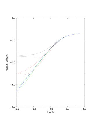
FIG. 2.: Cooling experiment in 1-D. 0.5-density versus temperature. We show the equilibrium value for density (continuous line) and the value for the density at different cooling rates. These are (from top to bottom) 0.1,0.01 and 0.001.

FIG. 3.: Cooling experiment in 3-D. 0.5-density versus temperature. We show the equilibrium value for density (continuous line) and the value for the density at different cooling rates. These are (from top to bottom) 0.1,0.01 and 0.001.

3 Heating Experiments

An striking feature of this system is that although no potential energy has been introduced there appear to be a large number of stable crystalline states at zero temperature which have an infinite lifetime. To see the effect of these crystalline states on the dynamics we have done some heating experiments. At $T=0$ an in 1-D, we have constructed different periodic crystalline initial conditions (putting the density every $p$ sites equal to one). As we have shown in section (II B), crystalline configurations with $p=2,3$ are metastable states at zero temperature. Numerically we find that the configurations where $p=4$ and $p=6$ decay to the configuration $p=2$, and that $p=5$ and $p=7$ does not decay to $p=2$ or $p=3$, but to solutions with densities between $\frac{1}{2}$ ($p=2$) and $\frac{1}{3}$ ($p=3$). These results are simply explained noting that, although the restriction $\sigma_{2}=0$ is a global one, apparently the only way to fulfill this restriction is imposing that every occupied site is surrounded by empty sites.

At finite temperature, the metastable states have a finite lifetime and decay to the equilibrium state. However, at low temperatures, the lifetime of metastable states can be very large and their effects on the dynamics can then be observed. Suppose we prepare the system in such a way that the initial condition belongs to the basin of attraction of one of these stationary states. If we perform a heating experiment in which we raise the temperature of the system at a finite rate, then we find that the system is trapped for some time near the basin of attraction. In figure 4, we show the case where we start from a non metastable state with $p=5$. We see that first it decays to the crystal state (the first plateau seen in the figure) an later on it relaxes to the equilibrium line.

FIG. 4.: Heating experiment in 1-D. 0.5-density versus temperature. Starting from a 5 period 1-D crystal initial condition. We show the equilibrium value for density (continuous line) and the value for the density at different cooling rates. These are (from top to bottom) 0.1,0.01, 0.001 and 0.0001.

4 Kinetic growth.

In the LP model, contrarily to the case of the spherical Sherrington-Kirkpatrick model [16], it is possible to investigate kinetic growth phenomena, i.e. how the condensed domains grow as time goes by. This is interesting because allows to ascertain how relevant is dimensionality in non equilibrium phenomena. Let us consider the densities in Fourier space eq.(17). Using equation (21) we obtain its time evolution,

$$\frac{1}{2}\frac{d\,|\tilde{\rho}({\bf k})|^{2}}{d\,t}=N\delta(k)\rho-\lambda_{0}(2|\tilde{\rho}({\bf k})|^{2}-N\delta(k)\rho)-4\lambda_{1}D\,|\tilde{\rho}({\bf k})|^{2}\gamma(k)+T$$ (62)

Integrating this equation with the values for the Lagrange multipliers obtained from the hierarchy of the density, we get the Fourier transformed densities for the infinite system. During the evolution from a non-equilibrium initial condition, we see how a peak around $k=\pi$ is formed (in 3-D, around ${\bf k}=(\pi,\pi,\pi)$). As temperature decreases the peak becomes sharper. For a better understanding of the results, we can appeal to the equilibrium relations. Using (23), (27) and (28) we can calculate an effective temperature for any $|\tilde{\rho}({\bf k})|^{2}$. Obviously, in equilibrium, all of them will have the same effective temperature, the equilibrium one.

In figure 5, we show the values of the effective temperature for values of ${\bf k}=k\,(1,1,1)$, with $k$ ranging from 0 to $\pi$ in the 3-D case (the figure is symmetric around $k=\pi$). For times larger than a typical time $t^{*}\simeq 1$ a plateau appears in the effective temperature and its value decays very fast to $T$, the temperature of the heat bath. For values of $k$ ranging from zero up to a given value $k_{max}$, all the modes have approximately the same effective temperature which is the equilibrium one [21]. There is a given value of $k$ (let us call it $k^{*}$) where the effective temperature becomes infinite and above this value of $k^{max}$ the effective temperature is not defined (This means that there does not exist an equivalent equilibrium system described by the dynamical densities $|\tilde{\rho}({\bf k})|^{2}$).

FIG. 5.: Effective temperatures versus k in 3-D and at $T=0.1$. It is shown for different values of time: 0.01,0.1,1,10,100,1000. The vertical line on the right of the plot is $k=\pi$.

With the value of $k_{max}$ we can also estimate the correlation length using the relation $\xi\simeq\frac{1}{\pi-k_{max}}$. We find that the correlation length diverges as $t^{\frac{1}{2}}$ typical of domain growth in ferromagnets with non conserved dynamics (figure 6).

The dynamics in the LP model can be intuitively understood in the framework of the kinetic growth scenario [22]. For times less than $t^{*}$ there is no plateau in the effective temperature because the system is nearly empty and the system is filling the lattice in a random and uncorrelated way. As soon as the density becomes large enough, any change of the density in a site of the lattice is correlated with that of the nearest neighbors and any change in the density requires a reorganization of the local densities inside a given domain. So, a critical and finite time $t^{*}$ is needed till the first domains appears. At times larger than $t^{*}$ correlated domains start to grow in time. At length scales smaller than the growing correlation length $\xi$ the system is in local equilibrium (the effective temperature is the equilibrium temperature) while it is completely disordered (the effective temperature is infinite) at larger length scales. The domain growth scenario is nicely reproduced in the LP model.

FIG. 6.: Inverse of the correlation length, $1/\xi$, against time in 3-D and at $T=0.1$ (dotted line) and 1 (dashed line). The straight lines show $t^{-1/2}$ behavior.

C Two Times Quantities.

1 The Correlation and Response Functions.

In this section, we are going to study the correlation and response functions in equations (47) and (48) with $x=0$. We consider the following normalized correlation function,

$$C_{norm}(t,t^{\prime})=\frac{C_{0}(t,t^{\prime},x=0)-\rho_{eq}^{2}}{C_{0}(t^{\prime},t^{\prime},x=0)-\rho_{eq}^{2}}=\frac{C_{0}(t,t^{\prime},x=0)-\rho_{eq}^{2}}{\rho_{0}-\rho_{eq}^{2}}$$ (63)

where $\rho_{0}$ is the initial density at time $t^{\prime}$ and $\rho_{eq}$ is the equilibrium density corresponding to the system at temperature $T$. In what follows we redefine the time variables $t^{\prime}=t_{w}$ and consider the behavior of correlation functions for different values of $t_{w}$.

Our results confirm the simplest Mode Coupling scenario where relaxation proceeds in two steps, the $\alpha$ and $\beta$ relaxation processes. A comment now seems to be appropriate. Originally Mode Coupling theory was devised to understand the equilibrium dynamics of liquids in the vicinity of the glass transitions. Götze and collaborators [7] have proposed a general mathematical framework for the understanding of equilibrium relaxational processes which take place in the vicinity of a bifurcation instability. The model we propose here is a very simplified version of the glass scenario where there is no discontinuity of the ergodicity parameter in the bifurcation point (i.e. at the condensation phase transition temperature). In fact, above $D_{l}=2$ the LP model exhibits a usual second order phase transition with classical critical exponents $\nu=1/(D-2),\eta=0$ ($D\leq 4$). The dynamical critical exponent is $z=2$ typical of mean-field theory. This implies that the relaxation time diverges close to the transition temperature $T_{c}$ like $\tau\sim(T-T_{c})^{-2/(D-2)}$. In the critical point equilibrium time correlations decay like $t^{-(D-2)/z}$, i.e. like $t^{-1/2}$ for $D=3$. Among other results these scaling relations led naturally to the $1/t$ decay found in figure 1 for the density in all dimensions at the critical point and below it. Above $T_{c}$ the scaling behavior $C(t)\sim t^{-(D-2)/z}f(t/\tau)$ holds where $\tau$ is the divergent characteristic time scale and the superposition principle is then valid. We want to stress that, contrarily to other scenarios for glassy relaxations (see the discussion by Götze[23]) in this case there is only one relaxation process above $T_{c}$ since there is not discontinuity in the ergodicity parameter at $T_{c}$. But still it is quite interesting to investigate the extension of the Mode Coupling scenario to the off-equilibrium dynamics below $T_{c}$. In this case, it is necessary to consider the initial time dependence in the dynamical equations. This implies the emergence, among others, of new off equilibrium phenomena like aging, i.e. the dependence of the evolution of the system on the initial time state. Also below $T_{c}$ off-equilibrium correlation functions are expected to display the characteristic two steps form since the ergodicity parameter (i.e. the Edwards-Anderson parameter) is already finite.

We will consider $t_{w}$ larger than $t^{*}$, i.e. the typical time needed to reach a macroscopic density in the lattice starting from a nearly empty lattice. For values of $t_{w}<t^{*}$, the system is quite far from the asymptotic long time regime and obviously the two step form is hardly seen. There are qualitative differences between the 1-D and 3-D cases since in 3-D there is a condensed phase while the system is always disordered in the 1-D case. The off-equilibrium correlation function in 3-D decays in two steps: the $\beta$ process or stationary part with a decay to a plateau with a $t^{-1/2}$ and the slow $\alpha$ process where the density-density correlation function decays like $t^{-\frac{3}{2}}$. In the $\beta$ process the relaxation is stationary and depends only on the time difference $t-t_{w}$ while in the slow $\alpha$ process there is aging and the correlation functions depend on both $t$ and $t_{w}$ (figure 7). The scaling behavior $t/t_{w}$ is well reproduced in the off-equilibrium regime (figure 8). In 1-D the behavior is similar except for the plateau which is absent (only a small inflexion for the correlation function at short times is observed). In 3-D the plateau persists over an arbitrarily long time scale which grows with $t_{w}$ whereas for 1-D aging is interrupted and disappears when $t_{w}$ is of the order of the finite relaxation time.

FIG. 7.: Correlation function versus $t-t_{w}$ in 3-D at $T=0.1$. Different waiting times are shown. From top to bottom $t_{w}=10000$,1000,300,100,30,10,3,1.

FIG. 8.: Correlation function versus $(t-t_{w})/t_{w}$ in 3-D and T=0.1. Different waiting times are shown, $t_{w}=1000$,300,100,30,10,3,1. For times larger than 1, all of them merge in one curve except for $t_{w}=1$ (the lines on the left) which is too short.

The dynamical scenario in the LP model can be inferred from a study of the response function. In any dimension the response function decays very fast to zero showing no aging in the asymptotic long time regime. Indeed, in 3D we see that $G(t,t_{w})$ decays like $t^{-3/2}$ for long times and then the integrated response function decays as $t^{-1/2}$. This is an indication of the short-time memory of the system. In the context of glassy dynamics this indicates that the LP model has no anomaly in the response function [25].

FIG. 9.: Response function, $G(t,t_{w})$, versus $t-t_{w}$ in 3-D and for $T=0.1$. Different waiting times are shown. From top to bottom $t_{w}=10$,100,1000,10000.

D The Fluctuation Dissipation Theorem.

Once we know the values of the correlation and response functions, we can study the fluctuation-dissipation ratio,

$$X(t,t_{w})=\frac{G_{0}(t,t_{w})}{\frac{\partial C_{0}(t,t_{w})}{\partial t_{w}}}~{}~{}~{}.$$ (64)

This ratio is equal to 1 in equilibrium (recall that, by definition, a factor $T$ has been absorbed in the response function). Roughly, we find that $X(t,t_{w})$ is approximately equal to 1 for $t-t_{w}<t_{w}$, showing that the system is in local equilibrium in the stationary regime. For times $t-t_{w}$ larger than $t_{w}$ the $X$ decays to zero very fast. We find the same qualitative behavior in 1-D and 3-D. This is expected in the absence of anomaly since the response function decays very fast to zero in this regime. If we look more carefully (see figure 10), we find that there are two different regimes. For small values of $t_{w}$ ($t_{w}<t^{*}\simeq 1$ when the lattice starts to be filled of particles), the value of $X$ decreases monotonically; but for larger values of $t_{w}$, $X$ increases with $t$ until it reaches a maximum and after decreases very fast. Numerically, we can extrapolate that for $t_{w}$ tending to infinity and $t-t_{w}<t_{w}$ (i.e. in the $\beta$-regime) the $1-X(t,t_{w})$ tends to zero as $(t-t_{w})^{-1}$.

Using the fact that for long times the response functions decays as $t^{-3/2}$ and that the $X(t,t_{w})\simeq 1$, we can conclude that the correlation function decays to the plateau with a power law $t^{-1/2}$. This result has been checked directly by fitting the decay of the correlation function to the plateau (see below for an estimate of the value of the plateau) for large values of $t_{w}$.

FIG. 10.: 1-$X(t,t_{w})$ versus $t-t_{w}$. Different waiting times are shown. From top to bottom $t_{w}$=1,3,10,30,100,300,1000,10000. The straight continuous line shows $\frac{1}{t-t_{w}}$ behavior.

We can also study the evolution of $X(t,t^{\prime})$ as a function of $C(t,t^{\prime})$. Qualitatively we find very similar results in all dimensions: in the $\beta$-regime $X$ is close to 1 while in the $\alpha$-regime it decays very fast to zero. The 1-D and 3-D cases are depicted in figures 11 and 12 respectively. Interestingly enough in the 3-D case we also find (figure 12) that all the curves (except $t_{w}=1$ which is a too short time) cross at $C^{*}=C_{norm}(t,t_{w})\simeq 0.75$ (the value of $C^{*}$ increases for lower temperatures) corresponding to a value of $X^{*}\simeq 0.25$ . The value $C^{*}$ corresponds to the value of $C_{norm}(t_{w},t)$ in the plateau in the $\beta$-regime (see figure 7). It is possible to make all different curves (corresponding to different values of $t_{w}$) collapse in a universal one. We find that the scaling law,

$$X(t,t_{w})=X((C^{*}-C_{norm}(t,t_{w}))\,t_{w}^{0.4})$$ (65)

for $C_{norm}(t_{w},t)<0.75$ nicely fits data for all different values of $t_{w}$ (inset in figure 12). We can interpret naturally the value of $X$ in the two regimes as a ratio between the temperature of the system and an effective temperature $T_{f}$. For $C_{norm}(t_{w},t)>C^{*}$ we find $X\simeq 1$ and the effective temperature of the system coincides with the temperature of the thermal bath. In this $\beta$-regime the system is in local equilibrium. For $C_{norm}(t_{w},t)<C^{*}$ we find $X\simeq 0$ which means that the effective temperature is infinite. This is a confirmation of the results obtained in section V.B interpreted within the kinetic domain growth scenario. In that case it was found that the effective temperature outside equilibrated domains was also infinite. Note that the definition of an effective temperature is not free of inconsistencies in the most general case and there is not evidence a priori that both effective temperatures (in the $\alpha$ regime) for the one time quantities and the effective temperature obtained for the two time quantities coincide. A result of this type was found in the Backgammon model for the physical interpretation of the violation fluctuation dissipation ratio [24].

FIG. 11.: $X(t,t_{w})$ versus $C_{norm}(t,t_{w})$ in 1D at $T=0.0001$. Different waiting times are shown. From top to bottom $t_{w}=1000,300,100,10$.

FIG. 12.: $X(t,t_{w})$ versus $1-C_{norm}(t,t_{w})$ in 3-D at $T=0.1$. Different waiting times are shown. From bottom to top $t_{w}=1,3,10,30,100,300,1000,10000$. In the inset we show the collapse of the data using the scaling relation eq.(65) for various values of $t_{w}=30,100,300,1000$.

1 Correlation Between Replicas.

Up to now we have found qualitatively similar results in the off-equilibrium behavior in 1-D and 3-D. The question arises if it is possible to infer from the dynamics the existence of a condensed growing phase which could distinguish the 1-D from the 3-D behavior at finite T. It has been recently suggested [25] that it is possible to characterize the dynamical behavior in terms of the overlap between two replicas which start in the same initial configuration and follow different noise realizations. We have analyzed the quantity, $Q(t_{w},t)-Q_{eq}$ where $Q_{eq}=\rho_{eq}^{2}$ for different values of $t_{w}$. In a disordered phase we expect that $Q(t_{w},t)-Q_{eq}$ should decay to zero for long times because the two replicas depart one from each other even if they are at the same initial condition at $t_{w}$. This is the behavior we find in 1D (figure 13). In the 3-D case in the condensed phase (see figure 14) the situation is different. Now the two replicas remember they were in the same configuration at $t_{w}$ and do not depart indefinitely one from each other. The system is then constrained to follow something similar to gutters or channels in phase space [25]. Intuitively it is not difficult to interpret this result in terms of a domain growth process. We already now that the dynamics of the LP model is essentially dominated by the growth of correlated domains. In the 1-D case domains appear and disappear in time because the system is in the disordered phase. In this case the typical length of domains grow in time (we are at low temperatures) but domains can always appear and disappear. The pattern structure of domains is in some sense continuously changed in time. In the 3-D case, once domains start to grow, they are not destroyed again. During the condensation process the pattern structure of domains is essentially unchanged and it is only rescaled in time. Consequently the two-replicas overlap $Q(t_{w},t)-Q_{eq}$ does not decay to zero for long times.

FIG. 13.: Correlation between replicas, $Q(t,t_{w})-Q_{eq}$ against $t-t_{w}$ in 1D and $T=0.0001$. Different waiting times are shown. From top to bottom $t_{w}=1$,10,100,1000.

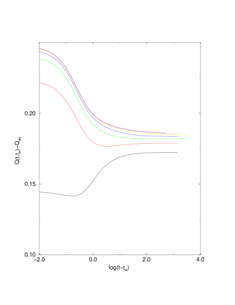
FIG. 14.: Correlation between replicas, $Q(t,t_{w})-Q_{eq}$ against total menus waiting time 3-D and $T=0.1$. Different waiting times are shown. From bottom to top $t_{w}=1$,3,10,30,100,300,1000.

VI Conclusions

We have analyzed in detail the dynamical properties of the LP model originally introduced to understand the thermodynamic properties of hard spheres lattice gases in the spherical approximation. From the viewpoint of the dynamics this is an interesting model because it is exactly solvable allowing a detailed investigation of the off-equilibrium scenario. The model has no built-in disorder and slow dynamics appears as a consequence of the short range dynamical constraints present in the system. The dynamics of this model shares a large number of features with the off-equilibrium dynamics of the spherical Sherrington-Kirkpatrick model [16] where dynamics is driven by the macroscopic condensation of the system on the disordered ground state. This gives support to the result that disorder is not an essential ingredient for the dynamical glassy scenario [3, 4] to be valid.

We have presented a detailed investigation of the dynamical equations of the model by considering the one time and two time quantities. One advantage of the model is that it includes short-range effects which are not present in other type of mean-field models like the spherical SK model [16]. If the initial configuration has density far from its equilibrium value then there is a short-time regime where the system is filled very fast in a spatially uncorrelated way. The typical time $t^{*}$ for this filling process is of order 1. It is only after that time that slow relaxation starts when the system is spatially correlated and needs to reorganize large regions in order to increase its density.

For values of time larger than $t^{*}$, we see that the dynamics of the model shows striking similarities to the kinetics of domain growth of ferromagnets with non conserved dynamics [22]. This is expected since the dynamics proposed in eq.(15) corresponds to the coarsening dynamics in the so called model B in phase ordering kinetics. In particular we have seen that for length scales smaller than a typical correlation length $\xi$ (which grows in time) the system is in local equilibrium and spatial fluctuations are determined by the equilibrium temperature. Above the correlation length $\xi$ the system is completely disordered, hence the typical temperature associated to spatial fluctuations is infinite. The correlation length $\xi$ is an accurate measure of the typical size of the growing domains. It would be interesting to investigate the dynamics of the LP model with the conserved dynamics of kinetic growth. In this case, we expect that a similar scenario would apply but with different exponents.

Further support to this domain growth scenario has been obtained from the study of the two time quantities. In particular we find that off-equilibrium relaxation proceeds in two well defined steps: a fast $\beta$ relaxation process where the fluctuation dissipation relation is obeyed, followed by a slow $\alpha$ process where time translation invariance is lost and the fluctuation dissipation ratio is zero. The physical meaning of the $\alpha$ and $\beta$ process is quite appealing in terms of domain growth kinetics. The fast $\beta$-process is associated to local rearrangements of densities inside domains whereas the slow $\alpha$-process is associated to the growth of the typical size of these domains. On the other hand, the response function shows no aging and decays very fast to zero. This is the scenario of glassy dynamics without anomaly in the response function typical of glassy systems with short term memory. A study of the replica-replica overlap has also revealed that the growth mechanism is different in the presence or absence of condensation transition. In 1-D where there is no condensation phase transition (the system is always in the disordered phase) the domains appear and disappear in time even if their typical size increases. In the 3-D case the domains always tend to grow and the pattern structure of domains is always maintained. In this last case we find that $\lim_{t_{w}\to\infty}\lim_{t\to\infty}Q(t_{w},t)$ is finite [25].

We want to note that the relaxation of the density as well as correlation functions do not display the phenomena of stretching characteristic of glasses. This is due to the oversimplification inherent to the model where only entropy barriers are introduced through global constraints (while in the classical hard-spheres model constraints are always local). It would be very interesting to introduce some kind of local constraint which could restore the main features observed in real glasses. In this direction, it would be quite interesting to extend this research by considering the LP model with the dynamics recently proposed by Dean where local densities can never become negative, a feature which is not considered in the present dynamics [26]. This requires the introduction of noise correlated with the local densities, a kind of local constraint. Also it would be interesting if such a dynamics could be exactly solved.

Acknowledgments. We acknowledge Luis Bonilla, Enrique Diez and Silvio Franz for stimulating discussions on this and related subjects. F. G. P acknowledges to the Universiteit van Amsterdam for the facilities during his stay there. The work by F.G.P. has been supported by the DGCyT The work by F.R has been supported by FOM under contract FOM-67596 (The Netherlands).

REFERENCES

- [1]
- [2] H. Rieger, Annual Reviews of Computational Physics II, p.295 (World Scientific, Singapore 1995); J. P. Bouchaud, L. F. Cugliandolo, J. Kurchan and M. Mezard, Out of Equilibrium dynamics in Spin Glasses and other Glassy systems Preprint cond-mat 9702070
- [3] J. P. Bouchaud and M. Mezard, J. Physique I (Paris) 4, 1109 (1994);
- [4] E. Marinari, G. Parisi and F. Ritort, J. Phys. A (Math. Gen.) 27 7615 (1994); J. Phys. A (Math. Gen.) 27 7647 (1994);
- [5] S. Franz and J. Hertz, Phys. Rev. Lett 74 2114 (1995).
- [6] T. R. Kirkpatrick and D. Thirumalai, Phys. Rev. B36 5388 (1987). T. R. Kirkpatrick and P. G. Wolynes Phys. Rev. B36 8552 (1987).
- [7] For review see, W. Götze, Liquid, freezing and the Glass transition, Les Houches (1989) J. P. Hansen, D. Levesque, J. Zinn-Justin editors, North Holland; W. Götze and L. Sjogren, Rep. Prog. Phys. 55, 241 (1992); C. A. Angell, Science, 267, 1924 (1995)
- [8] J. L. Lebowitz and J. K. Percus, Phys. Rev. 144, 251 (1966).
- [9] J. Zinn-Justin. Quantum field theory and critical phenomena. Oxford. Claredon Press, 1989, chap. 3.
- [10] G. H. Fredrickson and H. C. Andersen, Phys. Rev. Lett. 53, 1244 (1984); E. Follana and F. Ritort, Phys. Rev. B 54, 930 (1996).
- [11] L. F. Cugliandolo and J. Kurchan, Phys. Rev. Lett. 71 173 (1993); J. Phys. A (Math. Gen.) 27 5649 (1994);
- [12] Th. M. Nieuwenhuizen, Phys. Rev. Lett. 74 4293 (1995).
- [13] S. Franz and M. Mézard, Europhys. Lett. 26, 209 (1994); Physica A210, 48 (1994).
- [14] For a recent discussion see, R. Monasson and O. Pouliquen, Entropy of particle packings: an illustration on a toy model Preprint cond-mat 9702027.
- [15] T. H. Berlin and M. Kac, Phys. Rev. 86, 821 (1952).
- [16] J. M. Kosterlitz, D. J. Thoules and R. C. Jones; Phys. Rev. Lett. 36 1217 (1976).
- [17] S. Ciuchi and F. De Pascuale, Nucl. Phys. B 300 31 (1988); L. F. Cugliandolo and D. S. Dean, J. Phys. A (Math. Gen.) 28, 4213 (1995);
- [18] Compared to the usual definition of the response function both definitions differ only in a factor .
- [19] J. J. Brey and A. Prados, Physica A, 197, 569 (1993); J. J. Brey, A. Prados and M. J. Ruiz-Montero, J. Non-Cryst. Solids, 172-174, 371 (1994);
- [20] F. Ritort, Phys. Rev. Lett 75, 1190 (1995); S. Franz and F. Ritort, Europhys. Lett. 31, 507 (1995);
- [21] We have defined this as the value of in which the effective temperature is larger than the average value in the plateau
- [22] A. J. Bray, Adv. Phys. 43, 357 (1994)
- [23] W. Götze, J. Stat. Phys. 83, 1183 (1996).
- [24] S. Franz and F. Ritort, J. Phys. A (Math. Gen.) 30 L359 (1997).
- [25] A. Barrat, R. Burioni and M. Mezard, J. Phys. A (Math. Gen.) 29, 1311 (1996); A. Barrat, Ph. D. Thesis (Universite Paris VI), 1996.
- [26] D. Dean, J. Phys. A (Math. Gen.) 29, L613 (1996)