Distributions of Singular Values for Some Random Matrices

Abstract

The Singular Value Decomposition is a matrix decomposition technique widely used in the analysis of multivariate data, such as complex space-time images obtained in both physical and biological systems. In this paper, we examine the distribution of Singular Values of low rank matrices corrupted by additive noise. Past studies have been limited to uniform uncorrelated noise. Using diagrammatic and saddle point integration techniques, we extend these results to heterogeneous and correlated noise sources. We also provide perturbative estimates of error bars on the reconstructed low rank matrix obtained by truncating a Singular Value Decomposition.

In analysing large, multivariate data, certain quantities naturally arise that are in some sense ‘self averaging’, namely in the large size limit, a single data set can comprise a statistical ensemble for the quantity in question. One such quantity, the singular value distribution of a data matrix, is the subject of this paper. The Singular Value Decomposition (SVD) is a representation of a general matrix of fundamental importance in linear algebra that is widely used to generate canonical representations of multivariate data. It is equivalent to Principal Component Analysis in multivariate statistics, but in addition is used to generate low dimensional representations for complex multi-dimensional time series. One example is to generate effective low dimensional representations of high dimensional dynamical systems. Another example of curent interest is to de-noise and compress dynamic imaging data, in particular in the case of direct or indirect images of neuronal activity.

For most of the above applications it is important to understand the properties of an SVD of a matrix whose entries show some degree of random fluctuations. This has been achieved to an extent in multivariate statistics, where the sampling distributions of quantities associated with the PCA are computed; however, the computations involved are difficult and exact distributional results are limited.

In this paper, we use diagrammatic and saddle point integration techniques to obtain the densities of singular values of matrices whose entries have varying degrees of randomness. In particular, we study the problem in the asymptotic limit of large matrix size; this limit is well justified in realistic cases as will be described below. The density of SV’s has been obtained before, with other techniques, for matrices with each entry independently distributed normally with indentical variances [1, 2]. We are able to obtain distributions for some more general cases where the variances are not equal and/or correlations are present between matrix entries. Our results have implications towards isolating random components from image time series. Also, these results help in understanding the effects of truncating the SV spectrum at a given point, a technique that is widely applied to remove noise from data.

The SVD of an arbitrary (in general complex) $p\times q$ matrix ($p\geq q$) ${\cal M}$ is given by ${\cal M}=U\Lambda V^{\dagger}$, where the $p\times q$ matrix $U$ has orthonormal rows, the $q\times q$ matrix $\Lambda$ is diagonal with real, non-negative entries and the $q\times q$ matrix $V$ is unitary. Note that the matrices ${\cal M}{\cal M}^{\dagger}=U\Lambda^{2}U^{\dagger}$ and ${\cal M}^{\dagger}{\cal M}=V^{\dagger}\Lambda^{2}V$ are hermitian, with eigenvalues corresponding to the diagonal entries of $\Lambda^{2}$ and U and V the corresponding matrices of eigenvectors. Consider the special case of space-time data $I({\bf x},t)$. The SVD of such data is given by

$$I({\bf x},t)=\sum_{n}\lambda_{n}I_{n}({\bf x})a_{n}(t)$$ (1)

where $I_{n}({\bf x})$ are the eigenmodes of the spatial “correlation” matrix $C({\bf x},{\bf x}^{\prime})=\sum_{t}I({\bf x},t)I({\bf x}^{\prime},t)$, and similarly $a_{n}(t)$ are the eigenmodes of the “temporal correlation function” $C(t,t^{\prime})=\sum_{t}I({\bf x},t)I({\bf x},t^{\prime})$. If one considered the sequence of images as randomly chosen from an ensemble of spatial images, then $C({\bf x},{\bf x}^{\prime})$ would converge to the ensemble spatial correlation function in the limit of long times. If in addition the ensemble had space translational invariance then the eigenmodes $I_{n}({\bf x})$ would be plane waves $e^{i{\bf k}\cdot{\bf x}}$, the mode number “n” would correspond to wavevectors and the singular values would correspond to the spatial structure factor $S({\bf k})$. In general, the image ensemble in question will not have translational invariance; however the SVD will then provide a basis set analogous to wave vectors. In physics one normally encounters the structure factors $S({\bf k})$ that decay with wave vector, and in the more general case, the singular value spectrum, organized in descending order, will show a decay indicating the structure in the data.

We consider the case of a $p\times q$ matrix ${\cal M}={\cal M}_{0}+N$ where ${\cal M}_{0}$ is fixed and the entries of $N$ are normally distributed with zero mean. We consider below several cases of normal distributions for entries of $N$, including cases where there are correlations between entries of $N$. ${\cal M}_{0}$ may be thought of as the desired or underlying signal; for an SVD to be useful, ${\cal M}_{0}$ should effectively have a low rank structure.

It is convenient to work in terms of the resolvent

$${\cal G}(z)=Tr[(z-{\cal M}^{\dagger}{\cal M})^{-1}]=\sum_{n}{1\over z-\lambda_{n}^{2}}$$ (2)

where ${\cal G}(z)$ is a complex function. The density of SV’s is given by

$$\rho(\lambda)=\sum_{n}\delta(\lambda-\lambda_{n})={2\lambda\over\pi}\lim_{\epsilon\rightarrow 0}Im\Bigl{[}{\cal G}(\lambda^{2}-i\epsilon)-{\cal G}(\lambda^{2}-i\epsilon)\Bigr{]}$$ (3)

We proceed by finding a closed equation for the average of ${\cal G}(z)$ in the limit where $p,q\rightarrow\infty$ and $\sigma_{i}\rightarrow 0$ such that the variance of a matrix entry times q, $\sigma^{2}q$ converges to a finite limit $\tilde{\sigma}^{2}$ and $p/q$ is held fixed. The density of states is expected to be a self averaging quantity. Thus although we compute results by averaging over the ensemble, we expect to be able to apply our results to the SVD of individual data matrices.

To illustrate the method, consider the simplest case, where each element of the matrix is i.i.d. normally as ${\cal N}(0,\sigma)$. Since

$${\cal G}(z)=\partial_{z}\ln\det(z-{\cal M}^{\dagger}{\cal M})$$ (4)

the average of the resolvent over the probability distribution of the matrix ${\cal M}$ can be obtained from $\langle\ln\det(z-{\cal M}^{\dagger}{\cal M})\rangle$, which in turn may be computed using replicas. We introduce $n$ replicas of $q$ dimensional real vectors $X_{\alpha}=(x_{\alpha 1},..,x_{\alpha q})(\alpha=1,..,n)$. Consider the following identity

$$Z_{n}=\int\bigl{[}\Pi_{\alpha=1}^{n}\Pi_{a=1}^{q}\bigr{]}\Bigl{\langle}exp\bigl{(}-{q\over 2}\sum_{\alpha=1}^{n}X_{\alpha}^{T}(z-{\cal M}^{\dagger}{\cal M})X_{\alpha}\bigr{)}\Bigr{\rangle}=({2\pi\over q})^{nq\over 2}\langle\bigl{[}\det(z-{\cal M}^{\dagger}{\cal M})\bigr{]}^{-{n\over 2}}\rangle$$ (5)

One obtains the desired quantity from the above by taking $n\rightarrow 0$. Before computing the expectation over ${\cal M}$ in $Z_{n}$, we decouple the term $X_{\alpha}^{T}{\cal M}^{\dagger}{\cal M}X_{\alpha}$ using the Hubbard-Stratanovich transformation by introducing another $n$ vectors $Y_{\alpha}=(y_{\alpha 1},..,y_{\alpha p})(\alpha=1,..,n)$ which are $p$ dimensional. Performing the average over ${\cal M}$, we obtain

$$Z_{n}=({q\over 2\pi})^{np\over 2}\int\bigl{[}\prod dXdY\bigr{]}\exp\Bigl{(}-{q\over 2}\bigl{[}\sum_{\alpha}(zX_{\alpha}^{T}X_{\alpha}+Y_{\alpha}^{T}Y_{\alpha})-\tilde{\sigma}^{2}\sum_{\alpha\beta}X_{\beta}^{T}X_{\alpha}Y_{\alpha}^{T}Y_{\beta}\bigr{]}\Bigr{)}$$ (6)

Now, we decouple $\sum_{\alpha\beta}X_{\beta}^{T}X_{\alpha}Y_{\alpha}^{T}Y_{\beta}$ by using two $n\times n$ matrices $[Q_{\alpha\beta}]$ and $[R_{\alpha\beta}]$ as follows:

$$Z_{n}=2^{-n^{2}}({q\over 2\pi})^{{np\over 2}+n^{2}}\int \bigl{[}\prod dXdYdRdQ\bigr{]}$$

$$\exp\Bigl{(}-{q\over 2}\bigl{[}\sum_{\alpha\beta}(X_{\alpha}^{T}(z\delta_{\alpha\beta}-\tilde{\sigma}^{2}Q_{\alpha\beta})X_{\beta}+Y_{\alpha}^{T}(\delta_{\alpha\beta}-iR_{\alpha\beta})Y_{\beta}+iQ_{\beta\alpha}R_{\alpha\beta})\bigr{]}\Bigr{)}$$

The integral over $R$ enforces the condition $Q_{\alpha\beta}=Y_{\alpha}Y_{\beta}^{T}$, giving us back the previous expression.

At this stage, we are in a position to write $Z_{n}$ as an integral over $Q$ and $R$ only, since we can do the integrals over $X$ and $Y$.

$$Z_{n}=2^{-n^{2}}({q\over 2\pi})^{-{nq\over 2}+n^{2}}\int\bigl{[}\prod dRdQ\bigr{]}\exp\Bigl{(}-{q\over 2}\bigl{[}\ln\det(z-\tilde{\sigma}^{2}Q)+{p\over q}\ln\det(1-iR)+itr(QR)\bigr{]}\Bigr{)}$$ (7)

Ideally one should take the $n\rightarrow 0$ limit first and then let $q\rightarrow\infty$. In order to be able to perform analytical computations, we have to take the limit in the reverse order . That this gives the correct answer is verified later by a direct diagrammatic method.

When $p,q\rightarrow\infty$, with $p/q$ fixed, the integral is dominated by some saddle point. We take the replica diagonal ansatz, consistent with all the symmetries.

$$Q_{\alpha\beta}=Q(z)\delta_{\alpha\beta}$$ (8)

$$R_{\alpha\beta}=iR(z)\delta_{\alpha\beta}$$ (9)

Then we have to minimize

$$S\bigl{(}Q(z),R(z)\bigr{)}=\ln(z-\tilde{\sigma}^{2}Q(z))+{p\over q}\ln(1-R(z))+Q(z)R(z)$$ (10)

with respect to $Q(z)$ and $R(z)$. Hence the equations,

$${1\over z-\tilde{\sigma}^{2}Q(z)}={1\over{\tilde{\sigma}^{2}}}R(z)$$ (11)

$${p/q\over 1-R(z)}=Q(z)$$ (12)

Using the fact that $Z_{n}\sim\exp\bigl{[}-nqS\bigl{(}Q(z),R(z)\bigr{)}\bigr{]}$ and 4, we get

$$G(z)=\langle{\cal G}(z)\rangle={q\over z-\tilde{\sigma}^{2}Q(z)}$$ (13)

so that $G(z)$ satisfies

$$G(z)={q\over z-{p\tilde{\sigma}^{2}\over q-\tilde{\sigma}^{2}G(z)}}$$ (14)

This equation can also be obtained from a direct diagrammatic resummation of $\Bigl{\langle}Tr{1\over z-{\cal M}^{\dagger}{\cal M}}\Bigr{\rangle}$ expanded in powers of ${1\over z}$. The diagrammatic representation of these terms are shown in Fig.1.

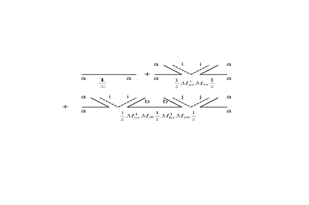
FIG. 1.: Diagrammatic representation of successive terms in the resolvent.

We use Wick’s theorem to take the average over $M$ with

$$\langle M_{ia}M_{jb}\rangle=\sigma^{2}\delta_{ij}\delta_{ab}$$ (15)

We have to concentrate only on the one-particle irreducible graphs, which give rise to the self-energy. The advantage of taking the large $p$,$q$ limit is that we have to consider only planar diagrams [3]. The diagrams contributing to self-energy, in the large $p$,$q$ limit are shown schematically in the Fig.2.

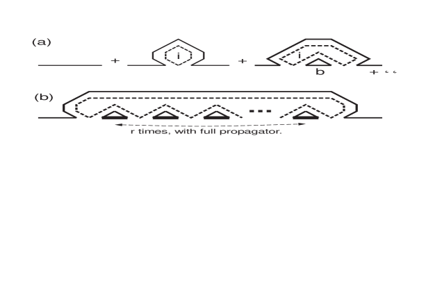
FIG. 2.: The diagrams that contribute to the self energy in large $p$, $q$ limit.

Summing the geometric series in this limit, we obtain

$$\Sigma(z)={p\tilde{\sigma}^{2}/q\over 1-\tilde{\sigma}^{2}G(z)/q}$$ (16)

$$G(z)={q\over z-\Sigma(z)}={q\over z-{p\tilde{\sigma}^{2}\over q-\tilde{\sigma}^{2}G(z)}}$$ (17)

The solution of this equation is

$$G(z)={1\over{\tilde{\sigma}}^{2}z}\bigl{[}-{\tilde{\sigma}}^{2}(p/q-1)+z\pm\sqrt{4p{\tilde{\sigma}}^{2}-(z-{\tilde{\sigma}}^{2}(p/q+1))^{2}}\bigr{]}$$ (18)

and

$$\rho(\lambda)={q^{1/2}\over\pi\lambda{\tilde{\sigma}}}\sqrt{(\lambda_{max}^{2}-\lambda^{2})(\lambda^{2}-\lambda_{min}^{2})}$$ (19)

for $\lambda_{min}<\lambda<\lambda_{max}$ and zero elsewhere.

$$\lambda_{max,min}={\tilde{\sigma}}\sqrt{(p/q+1)\pm 2\sqrt{p/q}}=\sqrt{2}\sigma\sqrt{(p+q)/2\pm\sqrt{pq}}$$ (20)

These results have been obtained by various authors (see for example [2]).

Generalising our methods, both the saddle point technique and the perturbative method, to the following cases is quite easy.

Case 1)

$$\langle M_{ia}\rangle=M_{ia}^{0}$$ (21)

The matrix $M^{0}$ has singular values $\lambda_{0a}$ where$a=1,\cdots,q$.

The covariance matrix is given as before by

$$\langle(M_{ia}-M_{ia}^{0})(M_{jb}-M_{jb}^{0})\rangle=\sigma^{2}\delta_{ij}\delta_{ab}$$ (22)

In this case we obtain

$$G(z)=\sum_{a=1}^{q}{1\over z-\lambda_{0a}^{2}-{p{\tilde{\sigma}}^{2}\over q-{\tilde{\sigma}}^{2}G(z)}}=G_{0}\Bigl{(}z-{p{\tilde{\sigma}}^{2}\over q-{\tilde{\sigma}}^{2}G(z)}\Bigr{)}$$ (23)

where

$$G_{0}(z)=Tr\Bigl{(}{1\over z-M^{0\dagger}M^{0}}\Bigr{)}$$ (24)

In case there are only few non-trivial $\lambda_{0a}$’s, $G(z)$ still satisfies a polynomial equation of order two or higher. Denby and Mallows [2] obtained similar results using a different method.

One of the simple consequences of eqn. 23 is the following. Consider a situation where there are only $r$ non-zero singular values of $M^{0}$, each of which is much bigger than the noise. Let the nonzero SV’s be $\{\lambda_{01},\ldots,\lambda_{0r}\}$. In the limit of zero noise,

$$G(z)=\frac{q-r}{z}+\sum_{a=1}^{r}\frac{1}{z-\lambda_{0a}^{2}}$$ (25)

In presense of finite small $\sigma$, the pole at zero broadens into a cut close to the origin, the other cuts develop around the nontrivial singular values which are far away from the origin.

Let us try to get the expression of $G(z)$ around the origin. For $z\sim{\tilde{\sigma}}$, ignoring terms of the order $({\tilde{\sigma}}/\lambda_{0a})^{2}$ for $a\leq r$, we find

$$G(z)\approx\sum_{a=r+1}^{q}{1\over z-{p{\tilde{\sigma}}^{2}\over q-{\tilde{\sigma}}^{2}G(z)}}=\frac{q-r}{z-{p\sigma^{2}\over 1-\sigma^{2}G(z)}}$$ (26)

which is just eqn. (17) with $q$ replaced by $q-r$, $\sigma$ (but not ${\tilde{\sigma}}$) remaining the same. Hence the smallest $q-r$ singular values have the same distribution as if they have come from a pure noise matrix which is of a smaller size, namely $p\times(q-r)$. This result is useful in fitting the formula to the tail of the singular value spectrum in a real data matrix, and is used in the fit displayed in Fig.3.

Case 2)

$$\langle M_{ia}\rangle=0$$ (27)

$$\langle M_{ia}M_{jb}\rangle=C_{ij}D_{ab}$$ (28)

$C$ and $D$ being $p\times p$ and $q\times q$ matrices. Such correlations may arise in imaging data when there is spatial inhomogeneity in the variance or spatial correlations due to filtering of an underlying uncorrelated spatial noise distribution, and/or when there is temporal filtering of data.

Here we consider

$$\tilde{G}(z)=\Bigl{\langle}{1\over z-M^{\dagger}M}\Bigr{\rangle}$$ (29)

Note that we did not take the trace, so that $\tilde{G}$ is a matrix.

We find that $\tilde{G}$ satisfies the equation

$$\tilde{G}(z)={1\over z-DTr{C\over 1-CTr(D\tilde{G}(z))}}$$ (30)

To the best of our knowledge, this is a new result. To see how to use it, let us consider two special cases.

a) When the noise variance differs from point to point in space.

$$\langle M_{ia}M_{jb}\rangle=\sigma_{a}^{2}\delta_{ij}\delta_{ab}$$ (31)

In this case,

$$\tilde{G}_{aa}(z)={1\over z-{\sigma_{a}^{2}\over 1-\sum_{b}\sigma_{b}^{2}\tilde{G}_{bb}(z)}}$$ (32)

which is a set of closed equations for$\tilde{G}_{aa}(z)$,$a=1,\cdots,q$.

b)There are non-trivial temporal correlations, introduced for example by linear filtering of an underlying uncorrelated process:

$$\langle M_{ia}M_{jb}\rangle=C_{ij}\delta_{ab}$$ (33)

Here

$$G(z)=Tr\tilde{G}(z)={q\over z-Tr{C\over 1-CG(z)}}$$ (34)

If the eigenvalues of $C$ are $\sigma_{i}^{2},i=1,\cdots,p$, then,

$$G(z)={q\over z-\sum_{i=1}^{p}{\sigma_{i}^{2}\over 1-\sigma_{i}^{2}G(z)}}$$ (35)

How do we obtain the singular value spectrum from Eq.35? One way is to rewrite it as

$$z=\frac{q}{G}-\sum_{i=1}^{p}\frac{1}{G-\frac{1}{\sigma_{i}^{2}}}$$ (36)

We want to know $G$ for real $z$. It is useful to first think of $z$ as a function of $G$ as defined in eqn.36 in the complex $G$ plane. We now look for level sets of $Im(z(G))$. By tracing the appropriate branch of the curve $Im(z(G))=0$, one can solve for $G(z)$ for real $z$. Taking the imaginary part of the function $G(z)$ thus found gives the density of singular values. The cumulative density of states, or equivalently the sorted singular values, can be found by integrating the singular value density.

Qualitative insight may be gained by realising that the real and the imaginary parts of z are the two components of the electric field in a $2$-dimensional electrostatic problem, with a charge $q$ at the origin, and point charges of strength $-1$ placed at each of the points $(1/\sigma_{i}^{2},0)$, $i=1,\ldots,p$ in the complex $z$ plane.

In addition to the density of singular values, one can try to compute the correlations between nearby singular values. It is well known in the theory of random matrices that the correlation functions of the eigenvalues of a random hermitian matrix has interesting universal features [4]. This is true for eigenvalues chosen from a small enough region, so that the eigenvalue density in that region is more or less constant. We find that the correlations of the singular values of a matrix, having each matrix element $iid$ distributed with mean zero and variance $\sigma^{2}$, are in the same universality class as the Gaussian Unitary Ensemble. The probability density $p(\Delta\lambda)$ of level spacings $\Delta\lambda$ goes as $\Delta\lambda^{2}$ for $\Delta\lambda<<\bar{\Delta\lambda}$. The probability density of $s=\Delta\lambda/\bar{\Delta\lambda}$ for the Gaussian Unitary Ensemble is well known in the Random Matrix literature [4]. It is possible that empirical level-spacing statistics can be used as a diagnostic to find out which singular values correspond mostly to ‘noise’ and which correspond mostly to ‘signal’.

So far, we have discussed what happens to the singular values. We would also like to estimate the errors made in reconstructing the matrix by keeping a small number terms in the left hand side of 1 which correspond to the biggest singular values. If we keep too few terms, we lose part of the signal. If we keep too many, we introduce back the noise. It would be useful to have expressions of the bias and the variance of the reconstruction. Unfortunately we do not have a simple extension of previous techniques to these calculations. Instead we compute these quanities for small sigma by doing a perturbative expansion.

Let us go back to case 1), namely when each element of the matrix $M$ is independently distributed with same variance $\sigma^{2}$ but different means. Let

$$M^{0}_{ia}=<M_{ia}>=\sum_{b}\lambda_{0b}u^{0b*}_{i}v^{0b}_{a}$$ (37)

and

$$M_{ia}=\sum_{b}\lambda_{b}u^{b*}_{i}v^{b}_{a}$$ (38)

We would like to calculate the mean and the variance of the variable $\hat{M}_{ia}=\sum_{b\in S}\lambda_{b}u^{b*}_{i}v^{b}_{a}$ where $S$ is a subset of $\{1,\ldots,q\}$.

For small $\sigma$,

$$<\hat{M}_{ia}> = \sum_{b\in S}\Bigg{[}\lambda_{0b}u^{0b*}_{i}v^{0b}_{a}+2\lambda_{0b}^{2}\sigma^{2}\sum_{c\neq b}\frac{\lambda_{0c}}{(\lambda^{2}_{0b}-\lambda^{2}_{0c})^{2}}u^{0c*}_{i}v^{0c}_{a}$$ (40)

$$-2\sigma^{2}\lambda_{0b}\sum_{c\neq b}\frac{\lambda^{2}_{0c}}{(\lambda^{2}_{0b}-\lambda^{2}_{0c})^{2}}u^{0b*}_{i}v^{0b}_{a}\Bigg{]}+o(\sigma^{4})$$

$$var(\hat{M}_{ia}) = \sigma^{2}\sum_{b\in S}\Bigg{[}|u^{0b*}_{i}v^{0b}_{a}|^{2}+\lambda^{2}_{0b}\sum_{j\neq b}\frac{(\lambda^{2}_{0b}+\lambda^{2}_{0j})}{(\lambda^{2}_{0b}-\lambda^{2}_{0j})^{2}}|u^{0j*}_{i}v^{0b}_{a}|^{2}$$ (42)

$$+\lambda^{2}_{0b}\sum_{c\neq b}\frac{(\lambda^{2}_{0b}+\lambda^{2}_{0c})}{(\lambda^{2}_{0b}-\lambda^{2}_{0c})^{2}}|u^{0b*}_{i}v^{0c}_{a}|^{2}-4\sum_{c\in S,c\neq b}\frac{(\lambda^{2}_{0b}\lambda^{2}_{0c})}{(\lambda^{2}_{0b}-\lambda^{2}_{0c})^{2}}|u^{0c*}_{i}v^{0b}_{a}|^{2}\Bigg{]}+o(\sigma^{4})$$

In this expression $j$ runs from $1$ to $p$ with $\lambda_{0j}=0,\mbox{for}j>q$.

To illustrate the utility of these results, we consider the SV distribution obtained from a space-time data set consisting of functional Magnetic Resonance Images (fMRI). The experimental details regarding the chosen data set can be found in [5]. For our purposes, the data constitutes a $1724\times 550$ matrix. The longer dimension corresponds to a subset of the pixels in a $64\times 64$ spatial image obtaining by discarding pixels which have intensity below a selected threshhold.

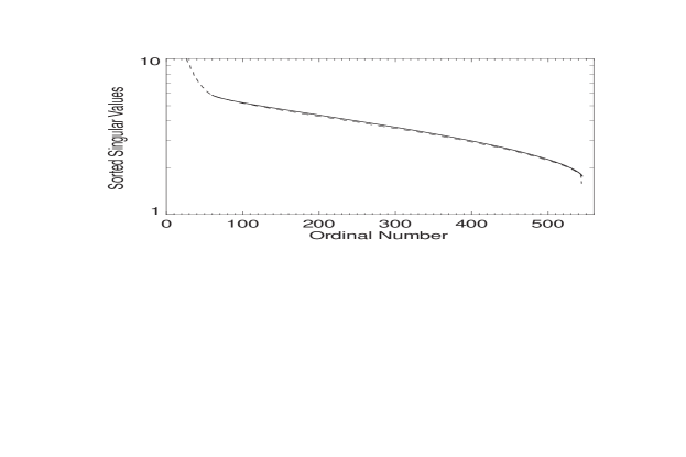
FIG. 3.: Comparison of singular values from a SVD of an fMRI data set with the theoretical formula for a noise only matrix.

In Fig.3, the tail of the SV distribution from this data is displayed along with a fit to a theoretical curve obtained from eqn.(19). The distribution has two adjustable parameters. One of them is the variance $\sigma$. A second adjustable parameter in the fit is the rank of the original matrix, which in this case has been assumed to be 60. We mentioned before that the effect of a few big singular values coming from the signal on the smaller singular values coming from the noise is an effective reduction of the dimensionality of the noise matrix. We fit the tail to the singular values of a $1724\times(550-60)$ pure-noise matrix. In fact, in the present case the uncorrelated noise can be estimated independently, and is therefore not really a free fitting parameter. We found that the fitted value of $\sigma$ is in close correspondence with the independently estimated value of the noise variance (data not shown).

In the example above, the good fit obtained between the theoretical curve and the tail in the SV distribution indicates that the noise entries in the original data were uniform and uncorrelated. It is easy to find experimental data where these conditions are violated, for example optical measurements of electrical activity in brain tissue [6] where the illumination is not fully uniform and the shot noise varies from point to point in space. Alternatively, the data may be spatially filtered and correlations may be introduced in space but not in time. Both of these cases produce SV distributions that cannot be fit by the procedure described above, but may be understood using eqn. (32). Details of these applications will be published elsewhere.

We acknowledge useful discussions with C. L. Mallows. One of us (AMS) was partly supported by the grant NSF DMR 96-32294.

REFERENCES

- [1] L. K. Hua, Harmonic Analysis of Functions of Several Complex Variables in the Classical Domains, American Mathematical Society, Providence, Rhode Island, 1963.
- [2] L. Denby and C. L. Mallows, “Computing Sciences and Statistics:Proceedings of the 23rd Symposium on the Interface”, E. M. Keramidas, Ed., 54-57, Interface Foundation, Fairfax Station, VA, 1991.
- [3] G. ’tHooft, Nucl. Phys. B72, 461 (1974).
- [4] M. L. Mehta, Random Matrices,Academic Press, New York,1991.
- [5] P. P. Mitra, S. Ogawa, X. Hu, K. Ugurbil, Mag. Res. Med. 37, 511 (1997).
- [6] J. C. Prechtl, L. B. Cohen, B. Pesaran, P. P. Mitra, D. Kleinfeld, PNAS 94, 7621 (1997).