Theoretical analysis of the experiments on the double-spin-chain compound – KCuCl₃

Abstract

We have analyzed the experimental susceptibility data of KCuCl₃ and found that the data are well-explained by the double-spin-chain models with strong antiferromagnetic dimerization. Large quantum Monte Carlo calculations were performed for the first time in the spin systems with frustration. This was made possible by removing the negative-sign problem with the use of the dimer basis that has the spin-reversal symmetry. The numerical data agree with the experimental data within 1% relative errors in the whole temperature region. We also present a theoretical estimate for the dispersion relation and compare it with the recent neutron-scattering experiment. Finally, the magnitude of each interaction bond is predicted.

The low-dimensional quantum systems with the excitation energy gap are now attracting much interest both experimentally and theoretically.[1] Possibility of the high-T_c superconductivity upon doping carriers to the gapped insulator lies as the background. The spin-ladder model and its realization in a real compound SrCu₂O₃ may be the most well-known substance for this scenario. [2] Of course, various other new compounds are also synthesized which can be explained by the low-dimensional quantum spin Hamiltonian. [3, 4, 5, 6, 7, 8] These experimental achievements now offer many data left for theoretical investigations.

Tanaka et al. [4] have measured the magnetic susceptibility of the KCuCl₃, and proposed that it can be explained by the double-spin-chain Hamiltonian. The susceptibility data show the spin-gap behavior. They estimated the amount of the excitation gap $\Delta$ by fitting the low-temperature data with its theoretical expression, $\chi(T)\propto T^{-1/2}\exp(-\Delta/T)$, given by Troyer et al.[9] The estimated gap, $\Delta/k_{\rm B}\sim 35$K, is consistent with their recent measurement of the magnetization process at low temperature, which gives $\Delta/k_{\rm B}\sim 31.1$K. [10]

For the thorough understandings of the system, we are necessary to determine the strength of each interaction bond of the model Hamiltonian which expresses the subject material. For frustrated systems, one usually calculates all the eigenvalues of a given model Hamiltonian on a finite lattice by the numerical diagonalization, and then compares the obtained physical quantities at finite temperatures with the experimental data. Since the numerical diagonalization technique is restricted to the very small sizes with sixteen $S=1/2$-spins or the less, the results suffer a severe finite size effect. The quantum Monte Carlo (QMC) method can handle much larger systems, but has not been applied to the frustrated systems because of the negative-sign problem. Recently, one of us (T. N.) has solved this problem in the double-spin-chain system.[11] It makes possible to treat large system sizes even at very low temperatures, and thus we are able to compare directly the numerical results to the experimental data without suffering the size effect.

In this Rapid Communication, we calculate the susceptibility of the double-spin-chain model with 162 spins, and aim at the determination of the interaction bonds that explain KCuCl₃. For this purpose, it is necessary to calculate the dispersion relation of the excited state to compare with the neutron-scattering experimental results. The susceptibility alone is not sufficient to discuss the details of the system, since it is the integrated quantity. We use our analytic expression for the dispersion relation obtained recently for general double-spin-chain models.[12] Our analysis partly disagrees with the experiments, which may be understood by possible two-dimensional couplings.

We consider the following spin Hamiltonian under the open boundary conditions:

$${\cal H}=\sum_{n=1}^{N-1}\Big{\{} J_{1} (\mbox{\boldmath$\sigma$}_{n}\cdot\mbox{\boldmath$\sigma$}_{n+1}+\mbox{\boldmath$\tau$}_{n}\cdot\mbox{\boldmath$\tau$}_{n+1})+J_{2}\mbox{\boldmath$\sigma$}_{n}\cdot\mbox{\boldmath$\tau$}_{n}$$ (1)

$$+ J_{3} \mbox{\boldmath$\tau$}_{n}\cdot\mbox{\boldmath$\sigma$}_{n+1}\Big{\}}+J_{2}\mbox{\boldmath$\sigma$}_{N}\cdot\mbox{\boldmath$\tau$}_{N}.$$ (2)

Here, $N$ is the linear size of the system, and $|\mbox{\boldmath$\sigma$}|=|\mbox{\boldmath$\tau$}|=1/2$. Figure 1 shows the shape of the lattice.

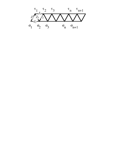
FIG. 1.: Shape of the general double spin-chain model.

Three cases of the above Hamiltonian, (i) $J_{1}=J_{3}$, (ii) $J_{3}=0$, and (iii) $J_{1}=0$, are especially investigated. In each case, $J_{2}$ is set variable ranging from $J_{2}=-8$ to $J_{2}=8$. The first one, $J_{1}=J_{3}$, is what we call here the ‘zig-zag’ or commonly called the railroad-trestle model. This model has frustration for $J_{2}>0$, and thus has not been analyzed on its thermodynamic properties yet. The second one is the ordinary two-leg ‘ladder’ model, and the third one is the ‘bond-alternation’ model. By changing the sign of the $J_{2}$-bond, the Hamiltonian can express both the dimer-gap system and the Haldane-gap system. Difference in the origin of the gap affects the structure of the excited states and thus the finite temperature behavior of various physical quantities. We also comment on this point at the end of this Rapid Communication.

Before the demonstration of the numerical evidences, we briefly summarize the simulational technique. We have done the ordinary world-line QMC simulations, but the choice of the representation basis is considered different from the conventional $s^{z}$ one. Two spins, $\mbox{\boldmath$\sigma$}_{n}$ and $\mbox{\boldmath$\tau$}_{n}$, are coupled and considered as a unit of update. This dimer unit takes four states associated with the $s^{z}$ eigenvalues of each spin, $|\sigma^{z},\tau^{z}\rangle$. We rearrange these four states so that they have the spin-reversal symmetry:

$$v_{1} = (|\uparrow,\uparrow\rangle+|\downarrow,\downarrow\rangle)/\sqrt{2},$$ (3)

$$v_{2} = (|\uparrow,\uparrow\rangle-|\downarrow,\downarrow\rangle)/\sqrt{2},$$ (4)

$$v_{3} = (|\uparrow,\downarrow\rangle+|\downarrow,\uparrow\rangle)/\sqrt{2},$$ (5)

$$v_{4} = (|\uparrow,\downarrow\rangle-|\downarrow,\uparrow\rangle)/\sqrt{2}.$$ (6)

Here, $\uparrow$ and $\downarrow$ denote the $s^{z}$ eigenstates. Now, two $J_{1}$-bonds and one $J_{3}$-bond just become a single effective bond connecting the neighboring dimer units, and a $J_{2}$-bond only contributes to the inner energy of a dimer unit. We can remove the negative-sign problem by using this representation basis. The Trotter number $m$ are chosen so that $\beta(2J_{1}+J_{3})/m$ varies from 0.35 to 0.15 at each temperature, and the extrapolations to the infinite $m$ are done. Typical number of the Monte Carlo steps is 500 000 divided into ten parts to see the statistical deviation. The first 50 000 steps are discarded for the equilibrium. The autocorrelation time of the susceptibility is less than an order of unity.

We have performed simulations for several values of $J_{2}$ in each choice of the $J_{1}$- and the $J_{3}$- bonds. First, we have set $J_{1}=J_{3}$ and done simulations thoroughly by changing a value of $J_{2}$ from $-8$ to $8$ in a step of 2. A rough estimate for the value of $J_{2}$ is made at this stage. Then, we have proceeded to the other cases, $J_{1}=0$ and $J_{3}=0$.

Figure 2(a) shows the QMC results of the susceptibility compared with the experimental data, and (b) is its low-temperature plot. The experimental data are the minimum susceptibility when the magnetic field is applied in the cleavage plane. The absolute value of the susceptibility depends upon the direction of the field, which can be understood by considering the anisotropy of the $g$-value.[4] Here, the $g$-value is determined by the comparison at high temperatures, $T>100$K. Error bars of the QMC data are almost negligible. Magnitude of each interaction bond is determined in order that the low-temperature data agree quantitatively with the experiment.

FIG. 2.: (a) The QMC results of the susceptibility (symbols) compared with the experimental data (line); (b) its low-temperature plot. The number of the spins is 162 and the open boundary conditions are used. The strength of each interaction bond is; ($\bigtriangleup$) Zig-zag: $J_{1}=J_{3}=8.35$K, $J_{2}=6J_{1}$, $g=2.05$, ($\circ$) Ladder: $J_{1}=12.3$K, $J_{3}=0$, $J_{2}=4J_{1}$, $g=2.05$, and ($\times$) Bond-alternation: $J_{3}=12.9$K, $J_{1}=0$, $J_{2}=4J_{3}$, $g=2.03$, respectively.

Triangles are the best fit to the experiment so far in the case of $J_{1}=J_{3}$, and the values of the interaction bonds are: $J_{1}=J_{3}=8.35$K, $J_{2}=6J_{1}$, i.e., all the interaction bonds are antiferromagnetic. The $g$-value $g=2.05$. Circles are those of the ordinary ladder case, and the values are: $J_{1}=12.3$K, $J_{3}=0$, $J_{2}=4J_{1}$, and $g=2.05$. Crosses are the case of the bond-alternation model: $J_{1}=0,J_{3}=12.9$K, $J_{2}=4J_{1}$, and $g=2.03$. All three data quantitatively agree with the experiment at all the temperatures. Our estimate for the $g$-value is also consistent with the ESR-measurement giving $g=2.05$.[10] Relative errors from the experiment are within $1\%$ in every case, and are smallest in the ‘ladder’ case. However, we are not sure the small deviations among three cases are relevant or not, because we have used a very-simplified model spin-Hamiltonian for a real compound. Systematic errors from an adoption of this model may be the most important one. Therefore, we cannot determine the strength of each interaction bond from the fitting of the susceptibility data alone. Only a common feature known from this plot is that the $J_{2}$-bond is strongly dimerized antiferromagnetically, and thus the origin of the gap is the dimer gap.

We try to determine the interaction bonds by the dispersion relation of the excitation energy now. This value is quite sensible to the details of the model. Recently, Kato et al. [13] applied the neutron-scattering analysis on this compound, and presented the dispersion relation. We compare our analytic dispersion relation with this experiment.

In our previous paper,[12] we have deduced an expression giving the dispersion of the general double-spin-chain systems as a function of the interaction bonds. There, we employed a single domain-wall variation after the non-local unitary transformation [14, 15] is applied. This approximation is quite excellent near $k=\pi$, checked with the numerical diagonalization results of finite systems, and with the exactly-known results. On the other hand, it becomes overestimated as the wave number $k$ approaches zero.

FIG. 3.: The dispersion relation of the excited states of the system. Zig-zag: $J_{1}=J_{3}=8.35$K and $J_{2}=6J_{1}$, Ladder: $J_{1}=12.3$K, $J_{3}=0$, and $J_{2}=4J_{1}$, and Bond-alternation: $J_{3}=12.9$K, $J_{1}=0$, and $J_{2}=4J_{3}$, respectively. The neutron-scattering experimental data are plotted by circles for the constant wave number perpendicular to the chain $k_{\perp}=0$, and by solid squares for $k_{\perp}=\pi$.

By using the values of the interaction bonds obtained from the susceptibility fitting, we give the dispersion of the excitation energy in Fig. 3. The first excitation is at $k=\pi$ in the ‘zig-zag’ and the ‘ladder’ models, and is at $k=0$ in the ‘bond-alternation’ model. Within our analysis, the first excitation is always at $k=\pi$ for $J_{1}>\min(J_{2},J_{3})/2$, and is otherwise at $k=0$, where $\min(J_{2},J_{3})$ stands for the minimum value of $J_{2}$ and $J_{3}$.

The dispersion of the ‘ladder’ case is consistent with the experimental dispersion parallel to the double chain when the constant wave number perpendicular to the chain $k_{\perp}$ is equal to zero. Our estimate of the gap is $\Delta/k_{\rm B}\sim 38$K, which is a little larger than the results of the magnetization process experiment. [10] So the ‘ladder’ model may be the most favorable candidate for explaining the KCuCl₃ at the present stage. However, it should be noticed that the experimental dispersion is dependent upon $k_{\perp}$. If a double-chain is isolated from each other, there should not be the $k_{\perp}$ dependences. Therefore, it might be an evidence of two-dimensional interaction couplings. This point is left for the future study.

Tanaka et al. [4] fitted their experimental data of the susceptibility to the theoretical expression $\chi(T)=(1/2\sqrt{\pi aT})\exp(-\Delta/T)$, given by Troyer et al. [9] supposing the form $\epsilon_{k}=\Delta+a|k-\pi|^{2}$ for the magnon dispersion. This expression is valid when $T\ll\Delta,D$, where $D$ is the band width of the magnon dispersion. If we take the effect of the band width into account, we obtain

$$\chi(T)={{\rm e}^{-\Delta/T}\over 2\pi\sqrt{aT}}\gamma\left({1\over 2},{D\over T}\right),$$ (7)

where $\gamma(x,p)$ is the incomplete gamma function defined by

$$\gamma(x,p)\equiv\int_{0}^{p}t^{x-1}{\rm e}^{-t}\,dt.$$ (8)

Since $D\ll\Delta$ from Fig. 3, $\chi(T)$ behaves as

$$\chi(T)\sim\cases{\displaystyle{{\rm e}^{-\Delta/T}\over 2\sqrt{\pi aT}}\left(1-\sqrt{T\over\pi D}{\rm e}^{-D/T}\right)&($T\ll D\ll\Delta$),\cr\displaystyle{1\over\pi}\sqrt{D\ \over a}{{\rm e}^{-\Delta/T}\over T}\left(1-{3D\over T}\right)&($D\ll T\ll\Delta$).\cr}$$ (9)

Thus, the expression of Troyer overestimates the susceptibility. In the fitting by Tanaka, the theoretical curve of Troyer severely deviates from the experimental curve for $T>20{\rm K}$, which is well-explained by $D=2.2\,{\rm meV}=25\,{\rm K}$ of the ‘ladder’ model.

In the last part of this Rapid Communication, we mention the difference of the susceptibility in the dimer-gap system and that in the Haldane-gap system. Only the ‘zig-zag’ case, $J_{1}=J_{3}$, is demonstrated as an example in Fig. 4. Product of the susceptibility and the temperature, $\chi T$, is plotted against the temperature, since this value is independent from the scale of the interaction bond. We use the logarithmic scale for the temperature axis, so that the rescaling of the temperature by changing the values of interaction bonds just causes a parallel shift along the temperature axis. Circles are the data of the dimer-gap system: $J_{1}=J_{3}=8.35$K, $J_{2}=6J_{1}$, $g=2.05$, and crosses are those of the Haldane-gap system: $J_{1}=J_{3}=45$K, $J_{2}=-4J_{1}$, $g=2.00$. These interactions are determined by fitting the low-temperature data, while the $g$-value is estimated at high temperatures. As seen from this figure, function form of $\chi T$ in the Haldane-gap system is obviously different from the experiment, so we cannot fit them by any parallel shift.

FIG. 4.: Product of the susceptibility and the temperature, $\chi T$, is plotted against the temperature. The QMC results of the dimer-gap system ($\circ$) and the Haldane-gap system ($\times$) are compared with the experimental data (line). The strength of each interaction bond is, ($\circ$) : $J_{1}=J_{3}=8.35$K, $J_{2}=6J_{1}$, $g=2.05$, and ($\times$): $J_{1}=J_{3}=45$K, $J_{2}=-4J_{1}$, $g=2.00$, respectively.

Let us consider the dimer limit, $J_{1}=J_{3}=0$, $J_{2}>0$, where the ground state is an array of independent singlet dimers and thus is non-degenerate. When the interactions between singlet dimers ($J_{1}$ and $J_{3}$) are introduced, the ground state is somewhat modified, but still has the nature of the singlet dimer. On the other hand, the ground state in the Haldane limit, $J_{1}=J_{3}=0$, $J_{2}<0$, is an array of independent triplet dimers and is highly degenerate. When $J_{1}$ and $J_{3}$ are switched on, the degeneracy is lifted up resulting in the unique ground state. The density of states of low-lying excited states are larger than the singlet dimer case, reflecting this high degeneracy of the ground state at $J_{1}=J_{3}=0$. Therefore, the susceptibility peak in the Haldane system becomes lower and broader than in the dimer system. We may determine the origin of the gap from the full width at half maximum of the susceptibility, or the function form of $\chi T$.

In summary, we have analyzed the susceptibility and the neutron-scattering measurements on the KCuCl₃ from the theoretical point of view. Large-scale quantum Monte Carlo simulations clarified this compound is well-explained by the double-spin-chain Hamiltonian with strong antiferromagnetic dimerization. Since the susceptibility alone is not sufficient to determine all the interaction-bond strengths, we also calculated the dispersion relation of the excited state to compare with the recent neutron-scattering experiment. As far as we restrict our theoretical analysis to the isolated double-spin-chain Hamiltonian, the best one to explain both measurements at present is the ladder model, which is defined by $J_{1}=12.3$K, $J_{2}=4J_{1}$, $J_{3}=0$, and $g=2.05$. This $g$-value agrees with the ESR-measurement.[10] However, the experimental dispersion relation has strong dependence on the constant wave number perpendicular to the chain, $k_{\perp}$, which cannot be explained by our theoretical analysis on the isolated double-spin-chain model. Thus, the system may have two-dimensional interactions that are not relevant at low temperatures.

The quantum Monte Carlo simulation has become the most realistic method to investigate the various quasi-one-dimensional compounds that can be expressed by the general double-spin-chain Hamiltonian even if the system has frustration. Present calculations can be extended to analyze other experiments easily. For example, we comment on that of Cu₂(1, 4-Diazacycloheptane)₂Cl₄ recently done by Hammar et al. [7] Their susceptibility data are consistent with our calculation down to the lowest temperature that could not be obtained by the numerical diagonalization. The choice of the interactions is $J_{1}=J_{3}=2.26$K, $J_{2}=6J_{1}$, and $g=2.04$.

Authors would like to thank H. Tanaka, T. Kato, and D. H. Reich for valuable discussions and for sending us the experimental data. They also acknowledge thanks to H. Nishimori for his diagonalization package Titpack Ver. 2, and to N. Ito and Y. Kanada for their random-number generator RNDTIK. A part of the computations were carried out on Facom VPP500 at the ISSP, University of Tokyo.

REFERENCES

- [1] For a review, E. Dagotto and T. M. Rice, Science 271, 618 (1996).
- [2] M. Azuma, Z. Hiroi, M. Takano, K. Ishida, and Y. Kitaoka, Phys. Rev. Lett. 73, 3463 (1994).
- [3] A. P. Ramirez, Ann. Rev. Mater. Sci. 24, 453 (1994).
- [4] H. Tanaka, K. Takatsu, W. Shiramura, and T. Ono, J. Phys. Soc. Jpn. 65, 1945 (1996).
- [5] M. Onoda and N. Nishiguchi, J. Solid State Chem. 127, 358 (1996).
- [6] K. Takatsu, W. Shiramura, and H. Tanaka, J. Phys. Soc. Jpn. 66, 1611 (1997).
- [7] P. R. Hammar, D. H. Reich, and C. Broholm, cond-mat/9708053.
- [8] D. A. Tennant, S. E. Nagler, T. Barnes, A. W. Garrett, J. Riera, and B. C. Sales, cond-mat/9708078.
- [9] M. Troyer, H. Tsunetsugu, and D. Würtz, Phys. Rev. B 50, 13515 (1994).
- [10] W. Shiramura, K. Takatsu, H. Tanaka, K. Kamishima, M. Takahashi, H. Mitamura, and T. Goto, J. Phys. Soc. Jpn. 66, 1900 (1997).
- [11] T. Nakamura, cond-mat/9707019.
- [12] T. Nakamura, S. Takada, K. Okamoto, and N. Kurosawa, J. Phys. Condens. Matter 9, 6401 (1997).
- [13] T. Kato, K. Takatsu, H. Tanaka, W. Shiramura, K. Nakajima, and K. Kakurai, preprint.
- [14] T. Kennedy and H. Tasaki, Phys. Rev. B 45, 304 (1992).
- [15] S. Takada and K. Kubo, J. Phys. Soc. Jpn. 60, 4026 (1991).