[

Simulations of Two-Dimensional Melting on the Surface of a Sphere

Abstract

We have simulated a system of classical particles confined on the surface of a sphere interacting with a repulsive $r^{-12}$ potential. The same system simulated on a plane with periodic boundary conditions has van der Waals loops in pressure-density plots which are usually interpreted as evidence for a first order melting transition, but on the sphere such loops are absent. We also investigated the structure factor and from the width of the first peak as a function of density we can show that the growth of the correlation length is consistent with KTHNY theory. This suggests that simulations of two dimensional melting phenomena are best performed on the surface of a sphere.

]

Halperin, Nelson [1] and Young [2] established several years ago a theory of defect–mediated melting of two dimensional (2D) crystals. It is based on ideas of Kosterlitz and Thouless [3]. It is envisaged that the transition from crystal to liquid takes place via two continuous transitions instead of the single first order melting transition of three dimensional crystals. A hexatic phase appears between ordered (solid) and isotropic (liquid) phases. We shall refer to this theory as KTHNY theory. The crystalline phase has both long-range crystalline order and bond orientational order, but the crystalline order is lost at the transition to the hexatic phase when according to KTHNY theory dislocation pairs unbind. As the temperature is raised further a second continuous transition occurs above which orientational order is lost when disclination pairs unbind and the isotropic liquid state forms. The correlation length $\xi$ over which there is short-range crystalline order diverges as $T$ approaches the melting temperature. It is given by the expression:

$$\xi(T)\propto\exp\left(\frac{b}{(T/T_{m}-1)^{\nu}}\right)$$ (1)

where $b$ is a numerical factor and $\nu=0.36963\ldots$

The KTHNY scenario is not the only mechanism possible for two-dimensional melting. It may happen that a single first order transition occurs before the defects unbind. Experimentally, there are systems to which the KTHNY theory applies and there are systems where just a single first order transition takes place. Electrons on the surface of helium [4], submicron polymer colloids confined between glass plates [5], structural order of two dimensional charge–density-waves in Nb_xTa_1-xS₂ [6] and colloidal particles confined to a monolayer with dipole interactions [7] are examples of the former while xenon on graphite [8] is a example of the latter.

However, Monte Carlo (MC) and molecular dynamics (MD) simulations of two dimensional melting almost always seem to indicate that melting takes place via a first order transition [9, 10, 11, 12]. Recently, there has been a very large scale simulation [13] of a system of particles interacting via a $r^{-12}$ potential with periodic boundary conditions. Systems of 4096, 16384 and 65536 particles were studied and as the number of particles increased the size of the van der Waals loops decreased implying that in the thermodynamic limit the melting transition might be continuous. It is the chief purpose of this paper to point out that it is much easier to get results valid in the thermodynamic limit by making the two-dimensional system live on the surface of a sphere.

Problems arise with MC and MD simulations when the relaxation times in the system become comparable with the timescale of the simulation. When plotting pressure versus density along an isotherm, a hysteresis loop can appear around the phase transition region. This is expected for systems with a first order transition but a system out of equilibrium can also show hysteresis. It has been found that deliberately introducing vacancies into the simulations with periodic boundary conditions decreases the jump at the first order transition [14]. This suggests that one of the problems of doing simulations with periodic boundary conditions is that the timescales employed in these simulations might be less than the timescale for nucleating defects such as vacancies, dislocation pairs etc. thus preventing the attainment of true equilibrium. Now on the surface of a sphere the crystalline state always contains at least 12 disclinations (i.e 5-fold coordinated sites) due to Euler’s theorem (see eg. [15]). Furthermore, dislocations appear even in the ground state to screen the 12 disclinations in order to reduce their elastic strain energy [15]. In other words, the topology of the sphere always forces a number of defects into the crystalline state. But instead of being a disadvantage as one might have first thought, the presence of the defects seems to allow the system to relax more readily and so explore more phase space on the timescale of the simulation. It is possible that this is the mechanism which makes simulations on the surface of a sphere closer to the thermodynamic limit than those done with periodic boundary conditions

Thermodynamic properties such as the free energy per particle for particles with short range interactions are the same on the flat plane and the sphere as $N\longrightarrow\infty$. When $N\longrightarrow\infty$ the local curvature vanishes ($R$, the radius of the sphere is varied with $N$ so as to keep the surface density $\rho$ constant) so that locally the system on the sphere appears flat.

We have studied by means of MD a system of $N$ particles constrained to move on the surface of a sphere. Particles interact with each other by the repulsive pair potential

$$v(r_{ij})=\epsilon(\sigma/r_{ij})^{12}$$ (2)

The distance $r_{ij}$ between particles $i,j$ is measured along the geodesic truncating at $r_{ij}=3\sigma$. $r_{ij}$ is given by the expression

$$r_{ij}=\vartheta_{ij}R$$ (3)

where $\vartheta_{ij}$ is the angle between particles $i$ and $j$.

$$\vartheta_{ij}=\arccos\left(\sin\theta_{i}\sin\theta_{j}\cos\left(\phi_{i}-\phi_{j}\right)+\cos\theta_{i}\cos\theta_{j}\right)$$ (4)

In this paper we will use reduced units ($\sigma=\epsilon=m=1$).

We employed a velocity Verlet algorithm. It was adapted to our particular case of polar coordinates $\theta_{i},\phi_{i}$ with $0\leq\theta_{i}\leq\pi$ and $0\leq\phi_{i}<2\pi$ for $i=1,2,\ldots N$;

$$\theta_{i}(t+\delta t) = \theta_{i}(t)+(v_{\theta_{i}}(t)\delta t+1/2a_{\theta_{i}}(t)\delta t^{2})R^{-1}$$ (5)

$$\phi_{i}(t+\delta t) = \phi_{i}(t)+\frac{2(v_{\phi_{i}}(t)\delta t+1/2a_{\phi_{i}}(t)\delta t^{2})}{\sin\theta_{i}(t+\delta t)+\sin\theta_{i}(t)}R^{-1}$$ (7)

where $a_{\phi_{i}}=\dot{v}_{\phi_{i}},a_{\theta_{i}}=\dot{v}_{\theta_{i}},v_{\phi_{i}}=R\sin\theta_{i}\dot{\phi_{i}},v_{\theta_{i}}=R\dot{\theta_{i}}$. Accelerations $a_{\phi_{i}},a_{\theta_{i}}$ for this problem are as follows

$$a_{\theta_{i}} = -\frac{12}{R^{13}}\sum_{j\neq i}^{N}\frac{\cos\left(\phi_{i}-\phi_{j}\right)\cos\theta_{i}\sin\theta_{j}-\cos\theta_{i}\cos\theta_{j}}{\vartheta_{ij}^{13}\sqrt{1-(\cos\vartheta_{ij}})^{2}}$$ (8)

$$a_{\phi_{i}} = \frac{12}{R^{13}}\sum_{j\neq i}^{N}\frac{\sin\left(\phi_{i}-\phi_{j}\right)\sin\theta_{j}}{\vartheta_{ij}^{13}\sqrt{1-(\cos\vartheta_{ij}})^{2}}$$ (10)

Temperature is introduced in the simulation by reselecting the velocities of all the particles at once according to a Boltzmann distribution. This reselection is done at equally spaced intervals of time[16].

It seems natural to choose values for $N$ such that the particles can be disposed on the sphere in a triangular–like lattice. This occurs when $N=10T+2$ where $T$ is equal to

$$T=h^{2}+hk+k^{2}$$ (11)

with $h$ and $k$ integers [17, 18]. For values of $N$’s satisfing Eq. (11) the particles can be arranged on the surface of the sphere into a state with full icosahedral symmetry. In this paper we study systems of 72, 122 and 272 particles.

It easy to see that the calculation of the accelerations from Eq. (LABEL:aceleraciones) is slower than the corresponding calculations on a flat plane as each element in the sum in (LABEL:aceleraciones) requires the (slow) computation of several trigonometric functions. This limits our simulation to rather small values of $N$, so it is fortunate that on the sphere results consistent with KTHNY theory can be seen with small values of $N$. The obvious idea of using look–up tables for the trigonometric functions led to considerable errors. We expect though that improvements in our numerical procedures can be found. This would allow us to study larger systems and so see the hexatic phase, which because it exists only in a narrow density region above the melting density, is hard to disentangle from finite size effects in small systems.

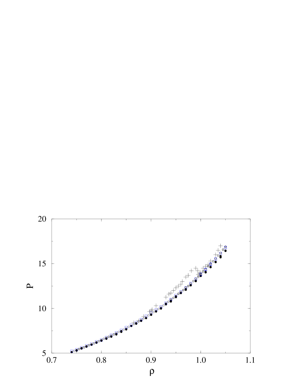
FIG. 1.: Pressure–density plot for 72 (solid circles), 122 (empty circles) and 272 (empty squares) particles on a sphere. Results from Broughton et al. (crosses) for the same potential on a flat plane are also plotted for comparison.

We have calculated the pressure $P$ and the structure factor along the isotherm $T=1$. A simulation time 400,000$\delta t$ was used for each value of the density, where $\delta t=0.005(m\sigma^{2}/\epsilon)^{1/2}$. The pressure was evaluated using the expression [19]

$$P=\rho k_{\rm B}T+\frac{6}{N}\sum_{i<j}^{N}\langle r_{ij}^{-12}\rangle$$ (12)

Fig. 1 shows the pressure–density isotherm for 72 (solid circles), 122 (empty circles) and 272 (empty squares). Crosses represent data obtained by Broughton et al.[9] for the same interacting potential on a flat plane. At low densities, the pressures are the same for the flat plane and for the sphere when both systems are closer to ideal gas behavior. As one can see in Fig. 1, there is no hysteresis loop on the sphere indicating that the solid phase does not melt by a first order transition.

If one concedes that there is no evidence for a first order melting transition then one might try to argue that what is happenning instead is that the topology of the sphere is preventing a solid phase forming and that the system is always liquid. However, by studying the structure factor we can see that a transition to a crystalline phase does indeed occur on the sphere.

The structure factor $S(k)$ is the Fourier transform of the pair correlation function $h(r)$. $h(r)$ is related to the pair distribution function $g(r)$ simply by $h(r)=g(r)-1$. Several authors have developed methods to calculate the structure factor in spherical geometries [20, 21]. We obtained it from the pair distribution function using the equation

$$S(k)=1+2\pi\rho R^{2}\int_{0}^{\pi}h(R\theta)\sin\theta J_{0}(kR\theta)d\theta$$ (13)

$J_{0}$ is the Bessel function of zeroth order. Fig. 2 shows the structure factor for $\rho=.9$. The dashed line is a Lorentzian fit to the first peak of the structure factor (which occurs at a wave-vector corresponding to the first reciprocal lattice vector of a triangular lattice). We define the inverse correlation length as the width of the first peak. Fig. 3 shows the behavior of the inverse width as a function of the density.

FIG. 2.: Structure factor for $\rho=0.9$ (solid circles). Dashed line is the Lorentzian fit used to obtain the width of the first peak. $a$ is a measure of the particle separation where $a=(\pi\rho)^{-1/2}$

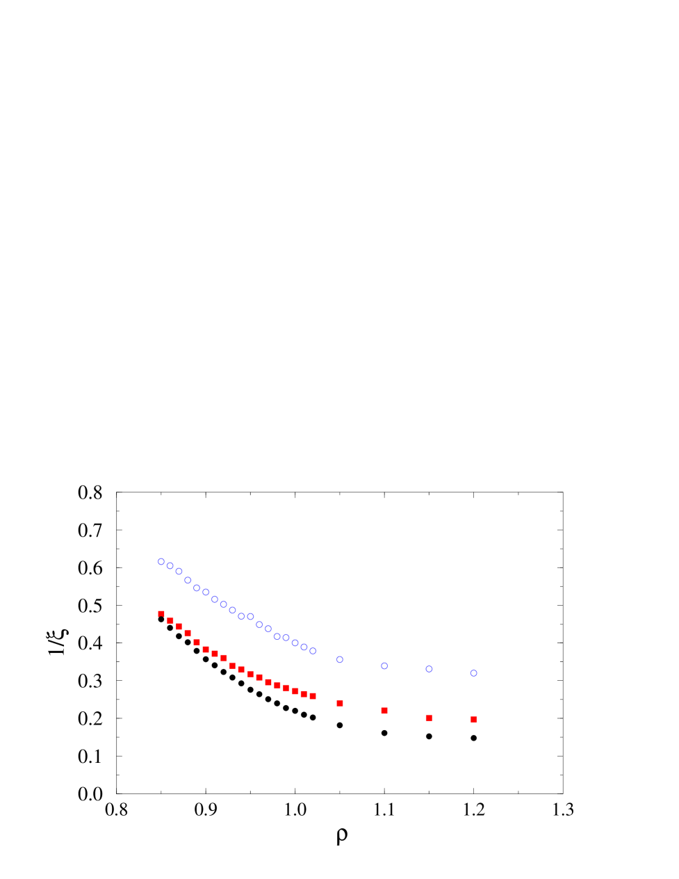
FIG. 3.: Width of the first peak of the structure factor, that is the inverse correlation length, as a function of density $\rho$. $N$ is equal to 72 (empty circles), 122 (solid squares) and 272 (solid circles)

$\xi$ saturates when $\rho\approx 1$ when $\xi$ is of the order of the radius $R$ of the sphere. This kind of behavior is as expected for a continuous phase transition.

Eq. (1) gives the dependence of $\xi$ in the liquid phase along an isochore. The dependence of $\xi$ along an isotherm is given by

$$\xi(\rho)\propto\exp\left(\frac{b}{\left((\rho_{m}/\rho)^{6}-1\right)^{\nu}}\right)$$ (14)

where $\nu=0.36963$ as before and $\rho_{m}$ is the melting density.

To obtain Eq. (14) from Eq. (1) we have used a scaling properties of the $r^{-12}$ potential [9]; viz that systems with different $T$’s and $\rho$’s share the same thermodynamic properties if they have the same value of $\Gamma$, where $\Gamma=(\pi\rho)^{6}/(k_{\rm B}T)$.

Fig. 4 shows a log–log plot of $\ln\xi$ as a function of $(1/\rho^{6}-1)^{0.36963}$. (We have taken $\rho_{m}=1$). A straight line of slope equal to -1 is also shown. This slope is the KTHNY prediction. The plot should thus should have a slope of -1 for densities approaching $\rho_{m}$ from below. (Very close to $\rho_{m}$ finite size effects will modify the behavior). The results obtained are clearly consistent with KTHNY theory, Eq. (14).

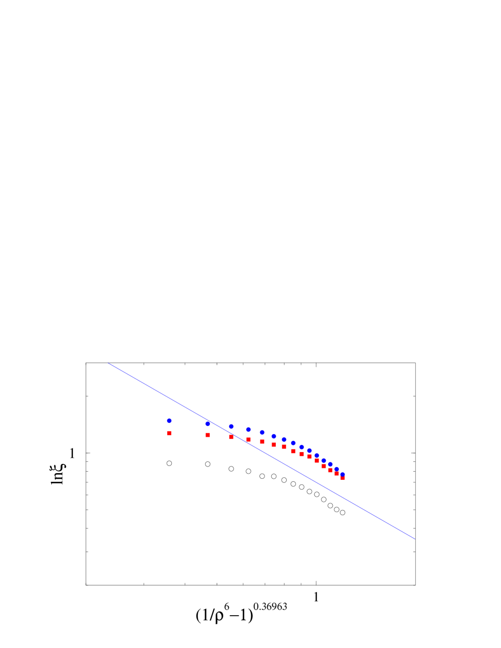
FIG. 4.: ln$\xi$ versus $(1/\rho^{6}-1)^{0.36963}$. The slope of the straight line is -1 which corresponds to KTHNY predictions. $N$ is equal to 72 (empty circles), 122 (solid squares) and 272 (solid circles)

To summarize, we have simulated a system of classical interacting particles on a sphere interacting via a short–range interaction. In this geometry there is no hysteresis loop as on a flat plane. By studying the structure factor, evidence of a continuous melting transition was found near $\rho=1$. The correlation length of short–range crystalline order in the liquid phase diverged on approaching the transition as predicted by KTHNY theory. We believe that this constitutes strong evidence that simulations of two dimensional melting phenomena are best performed on the surface of a sphere and implies that the first order transition so often reported in simulations on the flat plane is nothing but a numerical artifact.

We would like to acknowledge financial support from the Dirección General de Investigación Científica y Técnica, project number PB 93/1125, and a grant for APG. We also aknowledge useful discussions with A. Somoza and M. Ortuño.

REFERENCES

- [1] B. I. Halperin and D. R. Nelson, Phys. Rev. Lett. 41, 121 (1978)
- [2] A. P. Young, Phys. Rev. B 19, 1855 (1979)
- [3] J. M. Kosterlitz and D. J. Thouless, J. Phys. C, 6, 1181 (1973)
- [4] D. C. Glattli, E. Y. Andrei and F. I. B. Williams, Phys. Rev. Lett. 60, 1710 (1988)
- [5] C. A. Murray and D. H. Van Winkle, Phys. Rev. Lett. 58, 1200 (1987)
- [6] H. Dai C. M. Lieber, Phys. Rev. Lett. 69, 1576 (1992)
- [7] R. E. Kusner, J. A. Mann, J. Kerins and A. J. Dahm, Phys. Rev. Lett. 73, 3113 (1994)
- [8] A. J. Jin, M. R. Bjurstrom and M. H. W. Chan, Phys. Rev. Lett. 62 1372 (1989)
- [9] J. Q. Broughton, G. H. Gilmer and J. D. Weeks, Phys. Rev. B 25, 4651 (1982)
- [10] J. Tobochnik and G. V. Chester, Phys. Rev. B 25, 6778 (1982)
- [11] J. A. Zollweg and G. V. Chester, Phys. Rev. 46 11186 (1992)
- [12] J. Lee and K. J. Strandburg, Phys. Rev. B 46, 11 190 (1992)
- [13] K. Bagchi, H. C. Andersen and W. Swope, Phys. Rev. Lett. 76, 255 (1996)
- [14] K. J. Strandbourg, Rev. Mod. Phys. 60, 161 (1988)
- [15] A. Pérez–Garrido, M. J. W. Dodgson and M. A. Moore, Phys. Rev. B 56, 3640 (1997)
- [16] T. A. Andrea, W. C. Swope and H. C. Andersen, J. Chem. Phys. 79, 4576 (1983)
- [17] D. L. D. Caspar and A. Klug, Cold Spring Harbor Symp. Quant. Biol. 27, 1 (1962)
- [18] D. L. D. Caspar, Phil. Trans. R. Soc. Lond. A 343, 133 (1993)
- [19] M. P. Allen and D. J. Tildesley in Computer simulation of liquids, Oxford U. P., New York (1987)
- [20] J. A. O’Neill and M. A. Moore, Phys. Rev. B 48, 374 (1993)
- [21] J. P. Hansen, D. Levesque and J. J. Weis, Phys. Rev. Lett. 43, 979 (1979)