Ground state energy of the Hubbard model: cluster–perturbative results

Abstract

When electron correlations are important it is often necessary to use numerical methods to solve the Hamiltonian for a finite system (cluster) “exactly”. Unfortunately, such methods are restricted to small systems. We propose to combine the “exact” numerical diagonalization for small clusters with the perturbative calculations to take into account the intracluster as well as intercluster interactions.

I Introduction

Since the discovery of high–$T_{c}$ superconductivity [1], the behavior of strongly correlated electronic systems remains a central problem in contemporary condensed matter physics. In spite of considerable effort devoted to the analysis of these systems, it is clear that the necessary theoretical skills and tools to deal with strongly correlated fermion systems are lacking. There are no exact solutions except in one dimension (e.g., the $t-J$ model is exactly solved by the Bethe–ansatz method for $J=2t$ [2]) and approximate analytic techniques have been known to lead to qualitatively incorrect predictions. The fundamental obstacle which appears in the analytical approaches is the difficulty in handling the strong correlations in a satisfactory way. Moreover, in mean–field calculations it is necessary to make a priori assumptions about the ground–state properties.

Therefore, most work on models with strongly correlated electrons has been done using numerical techniques. Among others, variational calculations [3], various realization of quantum Monte Carlo simulations, [4] and an exact diagonalization of small systems [5] are used to obtain the properties of these models.

Unfortunately, numerical methods also meet some serious problems. The main difficulty in the quantum Monte Carlo calculations is the famous sign problem, which reduces the usage of this method at low temperatures and at the physically interesting densities. The minus sign problem does not arise in the diagonalization procedures, based on the Lanczös method [6] and its modifications [7], where all quantities (static and dynamical) can be computed from the ground state. Regretfully, the Lanczös technique is limited to small clusters by the rapid increase of the size of the Hilbert space with the number sites. Typically the calculations are performed on $4\times 4$ cluster with periodic boundary conditions for one hole, two holes, or an arbitrary number of holes. With respect to the infinite lattice this corresponds to an investigation of only a small number of points in the Brillouin zone. Therefore, the overall shapes of the energy bands cannot be determined precisely, and the influence of the cluster size on the eigenstates of the Hamiltonian can be important. The differences between results obtained for a finite cluster, and its values for an infinite lattice, are known as finite size corrections. It is often difficult to extrapolate the finite cluster data to the thermodynamic limit, and in certain cases it can lead to erroneous theoretical predictions. The corrections often do not decrease monotonically with the increase of the number of sites, mainly due to varying cluster geometries. Thus the estimation of finite size corrections by direct comparison of clusters of different sizes is difficult. Moreover, often one cannot compare different clusters with the same filling, as the number of sites as well as the number of electrons are integers.

There are various methods of minimizing the finite size corrections. The most obvious one, the increase of the size of the cluster, is strongly limited by the available time and memory of present–day computers. However, there have been some recent attempts to attack this problem, e.g., the diagonalization of the Hamiltonian in a reduced Hilbert space. [8] Another approach to finite size effects is based on a specific treatment of boundary conditions. Usually, when the hopping term in the Hamiltonian makes a particular jump out of the cluster, it is mapped back into the cluster through a translation without any change of the wave function. However, in order to reduce the finite size effects, twisted boundary conditions are sometimes used, i.e., the phase of the wave function is changed when the electron hops from one site to another. Then the properties of a larger system may be found by forming an average over smaller systems with different boundary boundary conditions [9]. In another method the boundary conditions are randomized by varying the magnitude rather then the phase of the “boundary” hopping.

The aim of the present work is to evaluate the ground state energy of the Hubbard Hamiltonian by employing yet another approach to the cluster calculations. Instead of applying some kind of boundary condition, we propose to mimic the infinite lattice by treating the electron hopping into or from a cluster as a small perturbation, and carrying out the summation of the perturbation series.

II Fundamentals of the Cluster–Perturbative (CP) Method

The idea of the present approach is to divide the infinite lattice into small exactly soluble clusters and consider the transfer between the clusters as a perturbation (see Fig. 1).

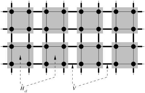
FIG. 1.: The lattice divided into clusters. $\hat{H}_{cl}$ are the cluster Hamiltonians and $\hat{V}$ is the terms describing the hopping between clusters.

The Hamiltonian of the system consists of two parts:

$$\hat{H}=\hat{H}_{cl}+\hat{V},$$ (1)

where

$$\hat{H}_{cl}=\sum_{I=1}^{\cal N}\hat{H}_{I}$$ (2)

is the sum of the cluster Hamiltonians, and

$$\hat{V}=\sum_{<IJ>}\hat{V}_{IJ}$$ (3)

describes the hopping between nearest neighboring clusters. ${\cal N}$ denotes the number of clusters.

The cluster Hamiltonian $\hat{H}_{I}\ (I=1,..,{\cal N})$ operates on the $I$th cluster’s Hilbert space ${\cal H}_{I}\ (\hat{H}_{I}:\ {\cal H}_{I}\rightarrow{\cal H}_{I})$ and the Hilbert space of the whole system is a direct product of the cluster’s Hilbert spaces ${\cal H}={\cal H}_{1}\otimes{\cal H}_{2}\otimes\ ...\otimes{\cal H}_{\cal N}$. Taking the size of the clusters relevant for numerical diagonalization, we are able to separately solve the cluster Hamiltonians. Now, in order to model the infinite lattice, we turn on the intercluster electronic transfer. The operator that moves electrons between clusters $I$ and $J$ ($I$ and $J$ are neighboring clusters) operates in a direct product of the Hilbert spaces of clusters $I$ and $J$:

$$\hat{V}_{IJ}:\ {\cal H}_{I}\otimes{\cal H}_{J}\rightarrow{\cal H}_{I}\otimes{\cal H}_{J}.$$ (4)

Assuming that the intercluster hopping energy is small compared to the distances between levels in the cluster’s spectrum, we can perform perturbation calculations, where the states of the Hamiltonian $\hat{H}_{cl}$ will be the zeroth-order approximation.

Let $\{|\phi^{I}_{i}\rangle\},\ i=0,1,...$ denote the set of states of $I$th cluster, and $\{\epsilon_{i}\}$ the corresponding energy levels $(\epsilon_{0}\leq\epsilon_{1}\leq\epsilon_{2}\leq...)$. Then

$$|\Phi_{\{i_{1},i_{2},..,i_{\cal N}\}}\rangle\,=\,|\phi^{1}_{i_{1}}\rangle\otimes|\phi^{2}_{i_{2}}\rangle\otimes...\otimes|\phi^{\cal N}_{i_{\cal N}}\rangle$$ (5)

is an eigenstate of $\hat{H}_{cl}$ corresponding to the energy

$$E_{\{i_{1},i_{2},..,i_{\cal N}\}}\,=\,\epsilon_{i_{1}}+\epsilon_{i_{2}}+..+\epsilon_{i_{\cal N}}.$$ (6)

The corrections to the ground-state energy $E_{0}$ in the $n$th order of the perturbation $\hat{V}$ are calculated summing the Goldstone diagrams

$$\Delta E_{n}\,=\,\langle\Phi_{0}|\,\hat{V}\left(\frac{1}{E_{0}-\hat{H}_{cl}}\hat{V}\right)^{n-1}|\Phi_{0}\rangle_{\rm conn},\ \ n=1,2,...\ ,$$ (7)

where $|\Phi_{0}\rangle\,\equiv\,|\phi^{1}_{0}\rangle\otimes|\phi^{2}_{0}\rangle\otimes...\otimes|\phi^{\cal N}_{0}\rangle$ is the ground state of the Hamiltonian $\hat{H}_{cl}$.

III Application of the CP formalism to Two-Dimensional Hubbard model.

On a simple square lattice, $\Delta E_{n}$ vanishes for odd $n$ since the perturbation $\hat{V}$ transfers an electron from one cluster to a neighboring one, and it needs an even number of jumps to return the electron to the outgoing cluster creating the ground state again.

The lowest-order nonvanishing contribution to the ground-state energy $\Delta E_{2}$ is given by:

$$\Delta E_{2}\,=\,{\sum_{i_{1},i_{2},..,i_{\cal N}}}^{\prime}\frac{{\bf|}\langle\Phi_{0}|\hat{V}|\Phi_{\{i_{1},i_{2},..,i_{\cal N}\}}\rangle{\bf|}^{2}}{E_{0}-E_{\{i_{1},i_{2},..,i_{\cal N}\}}},$$ (8)

where the prime means summing over all states excluding the ground state. In the case of simple square lattice the symmetry of the lattice allows to simplify this expression, leading to

$$\Delta E_{2}\,=\,2{\cal N}{\sum_{i_{1},i_{2}}}^{\prime}\frac{{\bf\mid}\langle\Phi_{\{0,0\}}|\hat{V}_{12}|\Phi_{\{i_{1},i_{2}\}}\rangle{\bf\mid}^{2}}{2\,\epsilon_{0}-\epsilon_{i_{1}}-\epsilon_{i_{2}}}.$$ (9)

The operator $\hat{V}_{12}$ is given by

$$\hat{V}_{12}=-t\sum_{\sigma}\left(a^{\dagger}_{3,1,\sigma}a_{4,2,\sigma}+a^{\dagger}_{2,1,\sigma}a_{1,2,\sigma}\right)+{\rm H.c.},$$ (10)

where we have used two indices for the creation and annihilation operators: the first indicates the position of a site within the cluster, and the second index is the number of the cluster. In Fig. 2 the solid lines connecting clusters 1 and 2 represent different terms of the operator $\hat{V}_{12}$ [Eq. (10)].

FIG. 2.: The hopping term which transfers electrons between clusters 1 and 2 ($\hat{V}_{12}$).

The matrix element $\langle\Phi_{\{0,0\}}|\hat{V}_{12}|\Phi_{\{i_{1},i_{2}\}}\rangle$ can be expressed in terms of $\langle\phi_{0}|a_{l,\sigma}|\phi_{i}\rangle$ and $\langle\phi_{0}|a^{\dagger}_{l,\sigma}|\phi_{i}\rangle$ ($\sigma=\uparrow,\downarrow;\ l=1,..,\cal{M}$, where $\cal{M}$ is the number of sites in the cluster), where $a_{l,\sigma}\ (a^{\dagger}_{l,\sigma})$ creates (annihilates) an electron with spin $\sigma$ on the $l$th site in the cluster. Thus all the calculations required to evaluate the second-order correction are performed within Hilbert space of a size equal to the size of Hilbert space of a single cluster.

In the same manner, we are able to take into account the fourth-order correction $\Delta E_{4}$. While the computational potential required to perform such calculations is much larger (mainly due to a summation over a large number of intermediate states), the Hilbert space is still the same as in the zeroth order. The general formula for the fourth-order correction is too complicated to be presented here. Instead, Fig. 3 shows all the diagrams that contribute to $\Delta E_{4}$ in the case of a simple square lattice.

FIG. 3.: The diagrams which contribute to the fourth order corrections.

The lines between clusters $I$ and $J$ represents a perturbation $\hat{V}_{IJ}$ that moves an electron between these clusters (in both directions, from $I$ to $J$ as well as from $J$ to $I$). The interaction in Eq. (7) operates on the ground state, and as a result also produces the ground state. Therefore, only diagrams of the forms of loops contribute to the ground-state energy and, for example, the following diagram does not appear in the fourth order: $\Box\!\rightarrow\!\Box\!\rightarrow\!\Box\!\rightarrow\!\Box\!\rightarrow\!\Box$. The simplest diagram (A) gives the contribution which can be written explicitly as

$$\Delta E^{A}_{4} = \Gamma_{A}\sum_{i_{1},i_{2}}\sum_{j_{1},j_{2}}\sum_{k_{1},k_{2}}\langle\Phi_{\{0,0\}}|\hat{V}_{12}|\Phi_{\{i_{1},i_{2}\}}\rangle$$ (11)

$$\times \langle\Phi_{\{i_{1},i_{2}\}}|\hat{V}_{12}|\Phi_{\{j_{1},j_{2}\}}\rangle$$ (12)

$$\times \frac{\langle\Phi_{\{j_{1},j_{2}\}}|\hat{V}_{12}|\Phi_{\{k_{1},k_{2}\}}\rangle\langle\Phi_{\{k_{1},k_{2}\}}|\hat{V}_{12}|\Phi_{\{0,0\}}\rangle}{(2\epsilon_{0}-\epsilon_{i_{1}}-\epsilon_{i_{2}})(2\epsilon_{0}-\epsilon_{j_{1}}-\epsilon_{j_{2}})(2\epsilon_{0}-\epsilon_{k_{1}}-\epsilon_{k_{2}})}.$$ (13)

A contribution from each diagram is multiplied by the factor which reflects the symmetry of the diagram and the lattice; for example there are four diagrams of type A (obtained by rotating diagram A around site 1 by $90^{\circ}$), and each one consists of two sites, so that $\Gamma_{A}=2$.

Equations for contributions from other diagrams are more complicated, for example diagram B includes the following processes:

$$1\rightarrow 2,2\rightarrow 3,3\rightarrow 2,2\rightarrow 1,\ \ \ 1\rightarrow 2,3\rightarrow 2,2\rightarrow 3,2\rightarrow 1,$$ (15)

$$2\rightarrow 1,2\rightarrow 3,3\rightarrow 2,1\rightarrow 2,\ \ \ 2\rightarrow 1,3\rightarrow 2,2\rightarrow 3,1\rightarrow 2,$$ (16)

$$1\rightarrow 2,2\rightarrow 3,2\rightarrow 1,3\rightarrow 2,\ \ \ 1\rightarrow 2,3\rightarrow 2,2\rightarrow 1,2\rightarrow 3,$$ (17)

$$2\rightarrow 1,2\rightarrow 3,1\rightarrow 2,3\rightarrow 2,\ \ \ 2\rightarrow 2,3\rightarrow 2,1\rightarrow 2,2\rightarrow 3,$$ (18)

where $I\rightarrow J$ describes the hopping from cluster $I$ to cluster $J$.

The summation over all intermediate states is a difficult, the most time–consuming task. In order to reduce the computational effort we have explicitly exploited various symmetries of the model. For example, calculating the matrix element $\langle\Phi_{\{i_{1},i_{2}\}}|\hat{V}_{12}|\Phi_{\{j_{1},j_{2}\}}\rangle$, conservation of the number of particles reduces the subspace of states $|\Phi_{\{j_{1},j_{2}\}}\rangle$ to $\left({\cal H}_{N(i_{1})+1}\otimes{\cal H}_{N(i_{2})-1}\right)\>\oplus\>\left({\cal H}_{N(i_{1})-1}\otimes{\cal H}_{N(i_{2})+1}\right)$ where ${\cal H}_{N}$ denotes a subspace of the cluster’s Hilbert space with $N$ electrons and $N(k_{m})$ is the number of electrons in the $k$th state on the $m$th cluster.

IV Results and Discussion

The second- and fourth-order corrections to the ground-state energy were calculated for different values of $U/t$ (for $n=1$). The results, presented in Fig. 4 and 5, are compared with the energies obtained by exact diagonalization of the Hamiltonian for $4\times 4$ system with periodic boundary conditions[10].

Generally, apart from the region of $U/t\leq 1$, where the perturbation series does not converge, the results from both these approaches are in agreement. The calculations were performed on IBM RS/6000 workstations, whereas diagonalization of $4\times 4$ clusters requires much larger computing facilities (see, e.g., Ref. [5]). The advantage of the CP approach, comparing to the exact diagonalization of larger systems is the lack of the memory limitations. With the increase of the order only the computational time increases, whereas the of size the diagonalized matrices is constant. Of course, this method, in contradiction to the standard Lanczös approach, does not allow a calculation of the dynamical properties of a given Hamiltonian. The formalism can be directly applied to systems described by other than Hubbard Hamiltonians, e.g., the $t-J$ model.

The most attractive application of the CP formalism is the study of the hole–hole effective interaction. Performing calculations for system with one and two holes in one cluster, while all the other clusters are with $n=1$, we can calculate the two–hole binding energy: $\Delta=E({\rm two\ holes})+E_{0}-2\,E({\rm one\ hole})$. Work in this direction is in progress. However, in the case of a doped cluster we have to perform the calculations for a degenerated spectrum, where the CPU and memory usage is much larger.

This scheme can be directly extended to a study of the nature of ground states of the undoped and doped systems.

FIG. 4.: The second and fourth order corrections to the ground state energy.

FIG. 5.: The comparison of ground state energy calculated using the CP approach with the result of Lanczös diagonalization of $4\times 4$ system.

REFERENCES

- [1] G.Bednorz, K.Müller, Z.Phys. B 64, 189 (1986)
-
[2]
P.Schlettmann, Phys.Rev. B 36, 5177 (1987)
P.–A.Bares, G.Blatter, M.Ogata, Phys.Rev. B 44, 130 (1991) -
[3]
H.Yokoyama, H.Shiba, J.Proc.Soc.Jpn. bf 57, 2483 (1988)
C.Gros, R.Joynt, T.M.Rice, Z.Phys. B 68, 425 (1987)
T.K.Lee, S.Feng, Phys.Rev. B 38, 11809 (1988)
R.R.P.Singh, M.Gelfand, D.A.Huse, Phys.Rev.Lett. 61, 2484 (1988) -
[4]
J.E.Hirsh, H.Q.Lin, Phys.Rev. B 37, 5070 (1988)
S.Sorella, S.Baroni, R.Car, M.Parinello, Europhys.Lett. 8, 663 (1989)
M.Imada, J.Phys.Soc.Jpn. 58, 2650 (1989)
S.R.White, D.J.Scalapino, R.L.Sugar, N.E.Bickers, R.T.Scaletter, Phys.Rev. B 39, 839 (1989) - [5] E.Dagotto, Rev.Mod.Phys. 66, 763 (1994)
- [6] J.K.Cullum, R.A.Willonghby, Lanczos Algorithms for Large Symmetric Eigenvalue Computation (Birkhauser, Boston 1985)
- [7] E.Dagotto, A.Moreo, Phys.Rev. D 31, 865 (1985)
-
[8]
J.Riera, E.Dagotto, Phys.Rev. B 48, 9515 (1993)
P.Prelovšek, X.Zotos, Phys.Rev. B 47, 5984 (1993) -
[9]
C.Gros, Z.Phys. B 86, 359 (1992)
C.Gros, Phys.Rev. B 53, 6865 (1996)
D.Poiblanc, Phys.Rev. B 44, 9562 (1991) -
[10]
E.Dagotto, A.Moreo, F.Ortolani, D.Poilblanc, J.Riera,
Phys.Rev. B 45, 10741 (1992)
G.Fano, F.Ortolani and A.Parola, Phys.Rev. B 42, 6877 (1992)