Abstract

Thermally activated escape of an over-damped particle from a metastable well under the action of a time-ramped force is studied. We express the mean first passage time (MFPT) as the solution to a partial differential equation, which we solve numerically for a model case. We discuss two approximations of the MFPT, one of which works remarkably well over a wide range of loading rates, while the second is easy to calculate and can provide a valuable first estimate.

Introduction – Thermally activated escape of a particle from a metastable well, has found numerous applications in a variety of systems[1]. Escape under the additional action of a time-dependent force constitutes a non-trivial generalization. Several studies [2, 3, 4, 5, 6] have been devoted to this problem for a sinusoidal force, which is particularly interesting since this system shows stochastic resonance [7]. The topic of the present paper is the effect of a time-ramped force on the escape rate. Apart from its fundamental significance, motivation to study this problem arises from recent work on the dynamical strength of molecular bonds [8, 9, 10]. The strength of a single bond can be measured experimentally using atomic force microscopy where one in practice applies a time-ramped force [8, 9, 11, 12, 13]. Evans and co-workers [8, 9] pointed out that the rupture strength of such a bond depends on the loading rate. This behavior has been seen not only in experiments but also in simulations of a Langevin equation [9, 10] and molecular dynamics simulations at very large loading rates [10, 14].

For the general problem of diffusive escape from a metastable well under a force that increases with time, we express the mean first passage time (MFPT) as the solution to a partial differential equation (pde). This exact approach differs from previous work that introduced an approximation based on instantaneous decay rates [9, 10]. The numerical solution of the exact equation is then compared with both this and another simple approximation. The first one works very well over a large range of loading rates. The second one can be calculated easily and still gives a reasonable estimate which is never off more than 30% over the entire range of loading rates.

MFPT as an exact solution to a pde – We consider the motion of an overdamped particle in a one-dimensional potential $V(x)$ under the action of a time-dependent force $f(t)$. The Langevin equation for this particle reads

$$\partial_{t}x=-V^{\prime}(x)+f(t)+\zeta,$$ (1)

where the stochastic noise obeys the usual correlations $<\zeta(t)\zeta(t^{\prime})>=2\delta(t-t^{\prime})$. Throughout the paper we measure energy in units of $k_{B}T$ and time and length such that the diffusion coefficient becomes 1. The potential $V(x)$ has a metastable well centered at $x=x_{m}$, a saddle point at $x_{s}$ and an activation energy $Q\equiv V(x_{s})-V(x_{m})$. While our approach holds for any $f(t)$, we will often specialize to a linear ramp

$$f(t)=\mu t$$ (2)

with loading rate $\mu$.

In the absence of the force ($f$=0), the MFPT $T(x)$ that a particle originally at $x$ needs to escape from this well obeys the equation [15]

$${\cal L}^{\dagger}T(x)\equiv(-V^{\prime}\partial_{x}+\partial_{x}^{2})T(x)=-1.$$ (3)

Here, ${\cal L}^{\dagger}$ is the backward Fokker-Planck operator. The boundary conditions are $T(x_{l})=T(x_{r})=0$, where for a metastable well $x_{l}$ is far to the left of the minimum and $x_{r}$ far to the right of the saddle point $x_{s}$. The explicit solution $T(x)$ as obtained by simple quadratures of (3) is well known [15, 16].

In the presence of a time-dependent force, relation (3) cannot be used without modification. To obtain an exact equation for the MFPT, one can get rid of the time dependence of the right hand side in (1) by writing this Langevin equation as a system of two equations

$$\partial_{t}x = -V^{\prime}(x)+f(\tau)+\zeta,$$ (4)

$$\partial_{t}\tau = 1.$$ (5)

In this form, the problem formally corresponds to a process homogeneous in time for the two variables $x(t)$ and $\tau(t)$. Therefore, one can apply the standard equation for the MFPT which becomes

$$(\partial_{\tau}+f(\tau)\partial_{x}+{\cal L}^{\dagger})T(x,\tau)=-1.$$ (6)

The boundary conditions in $x$ are as before $T(x_{l},\tau)=T(x_{r},\tau)=0$. Since the deterministic variable $\tau$ does not diffuse, the equation is first order in $\tau$. Therefore, one can specify only one boundary condition in $\tau$ which we choose as $T(x,\tau_{e})=0$. For these boundary conditions, the solution $T(x,\tau)$ gives the MFPT that the process (4) starting for $t=0$ at $x$ and $\tau$ needs to reach either one of the following boundaries: (i) the particle reaches the absorbing boundary at $x_{l}$ or $x_{r}$; or (ii) the variable $\tau$ becomes $\tau_{e}$. If $\tau_{e}$ is large enough, the number of events in which the particle has not reached the absorbing boundaries at $x_{l}$ or $x_{r}$ but rather that at $\tau=\tau_{e}$ are negligible compared to those in which it escapes over $x_{l}$ or $x_{r}$. Therefore, in the limit $\tau_{e}\to\infty$, the solution $T(x,\tau=0)$ gives the MFPT for the ramped problem. The argument $\tau=0$ arises from the fact that the ramping starts with $f(t=0)=0$ at $t=0$.

Escape rate for constant force – Before we present numerical solutions of (6), we discuss two approximations for the special case of a linearly ramped force $f(t)=\mu t$. To avoid a proliferation of symbols we use the same function symbol $T$ for all MFPT quantities under a time-varying force, it being unambiguous from the arguments which case is being discussed. Both approximations use the solution to the MFPT problem under constant force $f$, which we call $T_{0}(x,f)$, to construct approximate solutions for the MFPT under the time-varying force $f(t)=\mu t$. The MFPT $T_{0}(x,f)$ obeys

$$(f\partial_{x}+{\cal L}^{\dagger})T_{0}(x,f)=-1,$$ (7)

which is easily solved by quadratures as [15]

$$T_{0}(x,f)=[\int_{x_{l}}^{x}{dy\over\Psi(y)}\int_{x}^{x_{r}}{dy^{\prime}\over\Psi(y^{\prime})}\int_{x_{l}}^{y^{\prime}}dz\Psi(z)-\int_{x}^{x_{r}}{dy\over\Psi(y)}\int_{x_{l}}^{x}{dy^{\prime}\over\Psi(y^{\prime})}\int_{x_{l}}^{y^{\prime}}dz\Psi(z)]/\int_{x_{l}}^{x_{r}}{dy\over\Psi(y)},$$ (8)

with $\Psi(x)\equiv\exp(-V(x)+fx)$. These integrals will be calculated numerically.

A significant simplification occurs if one only requires the result (8) for large force-dependent activation barriers

$$Q(f)\equiv Q_{0}-f(x_{s}(f)-x_{m}(f))>>1.$$ (9)

A saddle point analysis of (8) then yields the well-known Kramers rate

$$T^{K}_{0}(f)=\tau_{0}(f)\exp[Q(f)].$$ (10)

The characteristic time

$$\tau_{0}(f)\equiv{2\pi\over[V^{\prime\prime}(x_{m}(f))V^{\prime\prime}(x_{s}(f))]^{1/2}},$$ (11)

is the inverse attempt frequency. $V^{\prime\prime}(x_{m,s}(f))$ is the curvature of the potential at the minimum and the saddle point, respectively, whose locations depend on the force $f$.

We use the numerical calculation of the MFPT under constant force (8), rather than the Kramers expression (10), to construct solutions for a time-varying force using two approximations. Both approximations thus obtained are valid for all applied forces even when $Q(f)>>1$ no longer holds.

Self-consistent constant force (SCCF) approximation – The idea of this crude approximation is that the escape is dominated by a typical force which is determied self-consistently. In the solution (8) for constant force we write $f=\mu T_{0}(x,f)$ which leads to the self-consistent relation $T=T_{0}(x,\mu T)$. Solving this equation yields the SCCF approximation $T_{s}(x,\mu)$. The main virtue of this simple approximation is that it can be calculated easily.

For large barriers, a further simplification can be achieved. Using the Kramers expression (10), the SCCF approximation $T_{s}^{K}(\mu)$ follows from solving the implicit equation

$$T^{K}_{s}(\mu)={2\pi\over(V^{\prime\prime}(x_{m})|V^{\prime\prime}(x_{s}))|^{1/2}}\exp(Q_{0}-\mu T^{K}_{s}(x_{s}-x_{m}))$$ (12)

where we notationally suppress the $f=\mu T^{K}_{s}$ dependence in $x_{m,s}=x_{m,s}(f)$.

Adiabatic approximation – A somewhat more refined approximation has been introduced previously within the context of stochastic resonance by Zhou et al [5] and for the ramped problem in Refs. [9, 10]. While the SCCF approximation focusses on the typical relevant force for the escape, the adiabatic approximation incorporates history dependence. It assumes a time-dependent escape rate $\nu(t)$. The probability that a given particle escapes at time $t$ is then given by

$$p(t)=\nu(t)\exp[-\int_{0}^{t}dt^{\prime}\nu(t^{\prime})].$$ (13)

Equation (13) says that the probability of rupture is the product of two terms: the instantaneous rupture rate $\nu(t)$ at a given time and the cumulative probability of survival up to that time. This approximation rests on the assumption that the escape process takes no time. In this limit it becomes exact. For the linear time-ramped process, one now replaces the time-dependence by a force-dependence via $f=\mu t$ which leads to the relation

$$p(f)=(1/\mu)\nu(f)\exp[-(1/\mu)\int_{0}^{f}df^{\prime}\nu(f^{\prime})].$$ (14)

Evans and Ritchie [9] discuss the conditions under which this probability has a peak at non-zero $f^{*}$, which is defined as the rupture force. Since within our approach, only the MFPT is available, we will discuss this quantity

$$T_{a}(x,\mu)=(1/\mu)\int_{0}^{\infty}df\exp-[(1/\mu)\int_{0}^{f}df^{\prime}\nu(f^{\prime})].$$ (15)

Since $\nu(f)=1/T_{0}(x,f)$ with $T_{0}(x,f)$ from (8), the MFPT $T_{a}(x,\mu)$ in the adiabatic approximation can be obtained by performing the two integrals numerically.

Numerical solution – In this section, we present numerical data which compare the MFPT obtained from the two approximations with the numerical solution of the exact equation (6).

Specifically, we use the potential

$$V(x)\equiv(27/4)Q_{0}x^{2}(1-x).$$ (16)

This potential exhibits a metastable minimum at $x_{m}=0$ with a saddle point at $x_{s}=2/3$ and an activation energy $Q_{0}$.

Fig. 1 shows the MFPT for two different values of the activation energy as a function of loading rate $\mu$ as calculated from (6). For $\mu=0$, the MFPT approaches the zero-force value as obtained from (3). The inset shows that over a large range $T\sim\mu^{-\alpha}$ where $\alpha\simeq 0.8$ is an effective exponent masking an extended crossover from $\alpha=1$ (with logarithmic corrections) to $\alpha=1/2$ as discussed below.

The quality of the two approximation is shown in Fig. 2, where we present the ratio of the MFPT

$$R_{a,s}(x,\mu)\equiv T_{a,s}(x,\mu)/T(x,\mu)$$ (17)

as calculated from either approximation to the exact value.

The gross features of these data can be understood by identifying three regimes [9, 10]. For small $\mu$, one expects naively that the MFPT deviates from the value at zero force if $\mu\raisebox{-3.22916pt}[-6.45831pt]{$\;\stackrel{{\scriptstyle>}}{{\sim}}\;$}\bar{\mu}$ where

$$\bar{\mu}\equiv Q(0)\exp[-Q(0)]/[\tau(0)(x_{s}-x_{m})].$$ (18)

While this (exponentially small!) loading rate also signifies the range where the SCCF starts to deviate from the exact data, the adiabatic approximation holds well even for larger loading rates. This is remarkable since as shown in the Appendix systematic perturbation theory reveals that both approximations fail to reproduce the $O(\mu)$ correction to the zero force result for a general potential. It seems that only in the additional limit of a large activation energy, $Q(0)>>1$, is good agreement between the exact result and the adiabatic approximation restored. A mathematical proof of this feature is beyond the scope of this paper.

For large $\mu$, both the potential and the diffusion can be ignored and then the ratio displayed in Fig. 2 can be calculated analytically. Even though the process in this regime is then no longer thermally-activated, we include it for two reasons. First, the MFPT is still mathematically well-defined and can even be calculated analytically in the limit $\mu\rightarrow\infty$. Second, for the bond rupture problem described in Refs. [9] and [10], this regime has some interest, where it has been called “ultrafast”. The time-ramped equation of motion becomes $\partial_{t}x=\mu t$ with the solution $x(t)=x+\mu t^{2}/2$. This leads to the exact asymptotic result

$$T(x,\mu)\approx\sqrt{2(x_{r}-x)/\mu}$$ (19)

and hence to $\alpha=1/2$ as mentioned above [17].

For the SCCF approximation, the equation of motion becomes $\partial_{t}x=f$, which leads to $T(x)=(x_{r}-x)/f$. Replacing $f$ by $\mu T(x)$ yields the relation

$$T_{s}(x,\mu)\approx\sqrt{(x_{r}-x)/\mu}$$ (20)

and hence $R_{s}(x,\mu)\approx\sqrt{2}/2$ for large $\mu$. In the same limit, the adiabatic approximation can be calculated by performing the integrals in (15). One obtains $R_{a}(x,\mu)\approx\sqrt{\pi}/2$ which is closer to the exact result than the SCCF approximation.

In an intermediate $\mu-$regime, the behavior can be extracted most easily from the SCCF approximation. From the relations $\ln T^{K}_{s}=\ln T^{K}(0)-\mu T^{K}_{s}(x_{s}-x_{m})$ one obtains $T_{s}^{K}\sim\ln\mu/\mu$ and thus $\alpha=1$ with logarithmic corrections. Expressed in terms of a mean rupture force $f^{*}\equiv T_{s}^{K}\mu$, this behavior corresponds to $f^{*}\sim\ln\mu$ [9]. As Fig. 1 shows, the data show a large crossover with an effective exponent $\alpha\simeq 0.8$.

Conclusions – In this paper, we have analysed diffusive escape over a barrier in the presence of a time-dependent force. We have derived an exact pde for the mean first passage time and solved it both by numerical integration and by use of two approximations. Comparison of the (numerically) exact solution with the adiabatic approximation introduced previously shows that this approximation holds remarkably well for a large range of loading rates. Formally, our exact equation for the MFPT can easily be generalized to include space-dependent diffusion coefficients. Likewise, both motion in higher dimensions and inclusion of inertia terms (for smaller friction) are amenable to the same treatment. The numerical solution of the corresponding equivalent of (6), however, will become quite time-consuming. It will then be helpful to explore the two approximations whose virtues we discussed for our model case.

Acknowledgments – U.S. thanks the Canadian Institute of Advanced Research and M. Bloom for the invitation to participate at a workshop where E. Evans gave a talk on this problem. Stimulating discussions with E. Evans, H. Gaub, M. Rief and M. Wortis are gratefully acknowledged.

A Small loading rates

For small $\mu$, perturbation theory of the SCCF approximation works out as follows. We first expand the solution of (7) as

$$T_{0}(x,f)=T^{(0)}(x)+fT^{(1)}(x)+O(f^{2}).$$ (A1)

The first order term obeys ${\cal L}^{\dagger}T^{(1)}(x)=-\partial_{x}T^{(0)}(x).$ We write its solution with the absorbing boundary conditions as $T^{(1)}(x)={\cal A}[-\partial_{x}T^{(0)}].$ The linear operator ${\cal A}$ can be expressed easily by quadratures and is formally the inverse to ${\cal L}^{\dagger}$. The final step consists in replacing $f$ by $\mu T^{(0)}(x)=\mu{\cal A}[-1]$. The first order result of the SCCF approximation thus reads

$$T_{s}(x,\mu)=T^{(0)}(x)+\mu{\cal A}[-1]\ {\cal A}[-\partial_{x}T^{(0)}]+O(\mu^{2}).$$ (A2)

A similar perturbative expansion for the adiabatic approximation shows that the term linear in $\mu$ coincides with the SCCF approximation whereas the terms $O(\mu^{2})$ differ in both approximations from each other.

Time (or rather $\tau$)-dependent perturbation theory in $\mu$ for the solution of the exact equation (6) can be set up as follows. Inserting the ansatz

$$T(x,\tau;\mu)=T^{(0)}(x)+\mu[T_{0}^{(1)}(x)+\tau T_{1}^{(1)}(x)]+O(\mu^{2})$$ (A3)

in (6), yields in $O(\mu,\tau^{1})$ the equation ${\cal L}^{\dagger}T_{1}^{(1)}=-\partial_{x}T^{(0)}(x)$ with the solution $T_{1}^{(1)}={\cal A}[-\partial_{x}T^{(0)}]$. Inserting this solution into the equation $O(\mu,\tau^{0})$ yields ${\cal L}^{\dagger}T_{0}^{(1)}=-T_{1}^{(1)}(x)$ with the solution $T_{0}^{(1)}(x)={\cal A}[-{\cal A}[-\partial_{x}T^{(0)}]]$. Thus, the full equation leads to the perturbative result

$$T(x,\mu)=T^{(0)}(x)-\mu{\cal A}[{\cal A}[-\partial_{x}T^{(0)}]].$$ (A4)

Since (A4) differs from (A2), neither approximation, perhaps somewhat surprisingly, reproduces the correct amplitude for the term linear in $\mu$. Note, however, that the $\mu=0$ value is reproduced by both approximations. We suspect that by considering the limit $Q\rightarrow\infty$ even the linear term shown in (A2) approaches the exact one shown in (A4), but we have not yet been able to show this mathematically.

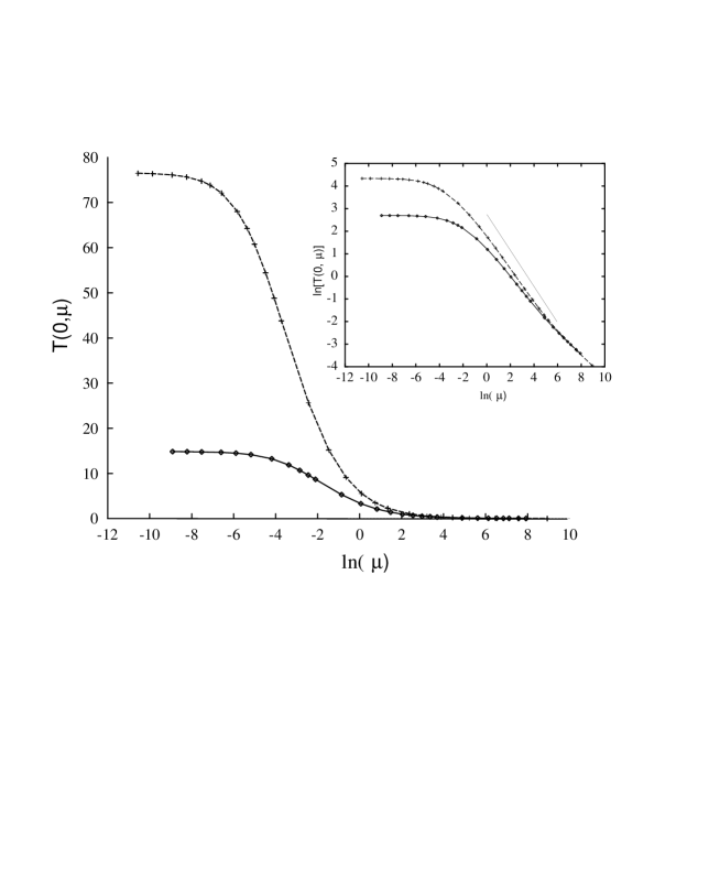
FIG. 1.: Mean first passage time $T(0,\mu)$ as a function of loading rate $\mu$ for $Q=7$ and $Q=5$ in the potential (16). Inset shows the same data logarithmically. For all $\mu$, the starting point has been chosen as $x=0$. The absorbing boundary is $x_{r}=1.6$ and the (quite irrelevant) left boundary is at $x_{l}=-1.6$.

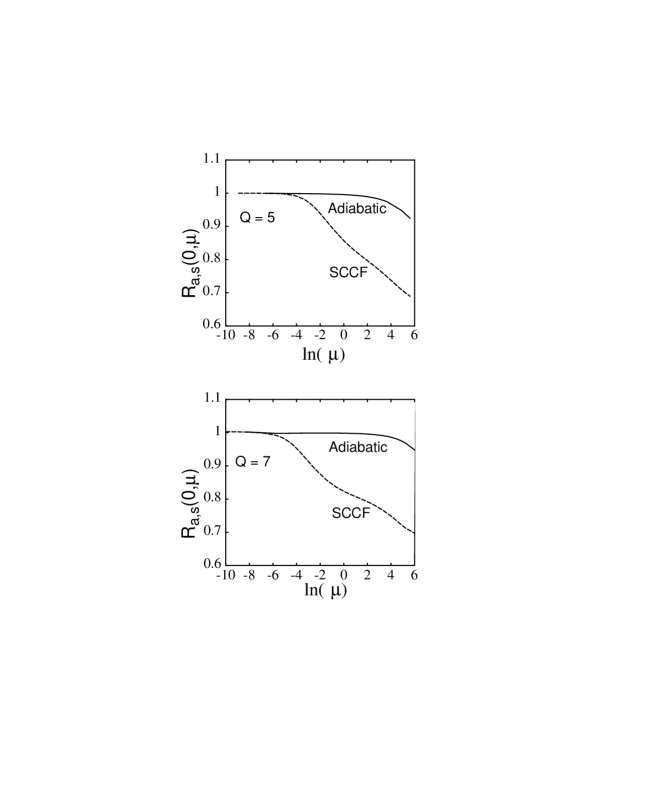
FIG. 2.: Mean first passage time $T(0,\mu)$ as a function of loading rate $\mu$ for $Q=7$ and $Q=5$ in the potential (16). Inset shows the same data logarithmically. For all $\mu$, the starting point has been chosen as $x=0$. The absorbing boundary is $x_{r}=1.6$ and the (quite irrelevant) left boundary is at $x_{l}=-1.6$.

REFERENCES

- [1] P. Hänggi, P. Talkner, and M. Borkovec, Rev. Mod. Phys. 62, 251 (1990).
- [2] R. F. Fox, Phys. Rev. A 39, 4148 (1989).
- [3] P. Jung and P. Hänggi, Europhys. Lett. 8, 505 (1989).
- [4] P. Jung, Z. Phys. B 76, 521 (1989).
- [5] T. Zhou, F. Moss, and P. Jung, Phys. Rev. A 42, 3161 (1990).
- [6] J. M. Casado and M. Morillo, Phys. Rev. E 49, 1136 (1994).
- [7] K. Wiesenfeld and F. Moss, Nature 373, 33 (1995).
- [8] E. Evans, D. Berk, and A. Leung, Biophys. J. 59, 838 (1991).
- [9] E. Evans and K. Ritchie, Biophys. J. 72, 1541 (1997).
- [10] S. Izrailev et al., Biophys. J. 72, 1568 (1997).
- [11] E.-L. Florin, V. T. Moy, and H. E. Gaub, Science 264, 415 (1994).
- [12] V. T. Moy, E.-L. Florin, and H. E. Gaub, Science 266, 257 (1994).
- [13] G. U. Lee, D. A. Kidwell, and R. J. Colton, Langmuir 10, 354 (1994).
- [14] H. Grubmüller, B. Heymann, and P. Tavan, Science 271, 997 (1996).
- [15] C. W. Gardiner, Handbook of stochastic methods for physics, chemistry and the natural sciences (Spinger, Berlin, 1994).
- [16] For a reflecting boundary at , some trivial modifications of subsequent formula will occur.
- [17] In this limit, the solution of Eq. 6 becomes , since formally . Setting then also leads to Eq. 19.