12 January 1998

Spin-spin correlation lengths of bilayer antiferromagnets

Abstract

The spin-spin correlation length and the static structure factor for bilayer antiferromagnets, such as YBa₂Cu₃O₆, are calculated using field theoretical and numerical methods. It is shown that these quantities can be directly measured in neutron scattering experiments using energy integrated two-axis scan despite the strong intensity modulation perpendicular to the layers. Our calculations show that the correlation length of the bilayer antiferromagnet diverges considerably more rapidly, as the temperature tends to zero, than the correlation length of the corresponding single layer antiferromagnet typified by La₂CuO₄. This rapid divergence may have important consequences with respect to magnetic fluctuations of the doped superconductors.

A powerful method to measure the spin-spin correlation length of a layered magnet is the neutron scattering method known as the energy integrated two-axis scan (TAS). In recent years, TAS has been successfully applied to La₂CuO₄[1], which is the parent compound of one of the high temperature superconductors. This experimental technique is not readily extendable, however, to a wide class of high temperature superconductors with close magnetic bilayers or triple layers within the unit cell; a particularly important example is ${\rm YBa_{2}Cu_{3}O_{6}}$, which has a close pair of magnetic planes within the unit cell, but it is otherwise a square lattice spin $S=1/2$ Heisenberg antiferromagnet. The reason for the difficulty is an intensity modulation[2] with the momentum transfer perpendicular to the planes. Thus, there have been no direct measurements of the correlation length despite considerable discussion of the importance of antiferromagnetic fluctuations in these materials.

In the present paper, we use both the field theoretical approach[3] and the numerical quantum Monte Carlo (QMC) loop algorithm[4] to obtain the low temperature properties of bilayer antiferromagnets. We also show that in the experimentally relevant regime TAS can be extended to such antiferromagnets. Thus, it is hoped that the antiferromagnetic fluctuations can be explored more thoroughly in future measurements. This is likely to be important in understanding the magnetic properties of the superconductors obtained by doping these antferromagnetic parent compounds.

The Heisenberg model for a spin-$S$ bilayer antiferromagnet is

$$H=J_{\parallel}\sum_{\langle ij\rangle,p}{\bf S}_{i}^{(p)}\cdot{\bf S}_{j}^{(p)}+J_{\perp}\sum_{i}{\bf S}_{i}^{(1)}\cdot{\bf S}_{i}^{(2)}.$$ (1)

The sum in the first term is over the nearest neighbor pairs on a square lattice in each plane, where the plane index $p$ takes two values 1 and 2. The second term represents the coupling between the planes. The exchange constants $J_{\parallel}$ and $J_{\perp}$ are both positive.

The low energy, long wavelength properties of the two dimensional Heisenberg model is well-described by the quantum $O(3)$ nonlinear $\sigma$-model[3]. Here, we shall consider its generalization to coupled bilayers. The Euclidean action for this system can be written down on general symmetry grounds[3], but it can also be derived from a $(1/S)$ expansion[5]. The action is

$$S = \int^{u}_{0}dx_{0}\int d^{2}x\Bigg{[}\sum_{p=1}^{2}\left({1\over 2g_{0}}|\partial_{\mu}\hat{{\bf\Omega}}^{(p)}|^{2}-h_{0}\sigma^{(p)}\right)$$ (2)

$$+ {1\over 2g_{\perp}^{0}}|\hat{{\bf\Omega}}^{(1)}-\hat{{\bf\Omega}}^{(2)}|^{2}-{1\over 2g_{t}^{0}}(\hat{{\bf\Omega}}^{(1)}\times\partial_{0}\hat{{\bf\Omega}}^{(1)})\cdot(\hat{{\bf\Omega}}^{(2)}\times\partial_{0}\hat{{\bf\Omega}}^{(2)})\Bigg{]},$$

where $\sigma^{(p)}$ is the component of the staggered field $\hat{{\bf\Omega}}^{(p)}$ in the direction of the staggered magnetic field $h_{0}$. Here, all the coupling constants and dimensional variables have been scaled to their dimensionless forms. We shall work directly at $d=2$; the label $\mu=1,2$ denotes the spatial directions, and $\mu=0$ denotes the imaginary time direction of extent $u$.

The relations between the $\sigma$-model parameters and the Heisenberg model parameters are known in the large-$S$ limit[5, 6], but we shall not need them in the present papper. The momentum cutoff of the $\sigma$-model, $\Lambda$, is chosen to be $\sqrt{2\pi}/a$, where $a$ is the lattice constant of the Heisenberg model, to conserve the number of degrees of freedom. The bare dimensional bilayer gap is given by $\Delta_{\perp}^{0}\equiv\hbar c_{0}\Lambda\sqrt{2g_{0}/g_{\perp}^{0}}$, where $c_{0}$ is the bare spin wave velocity at the scale $\Lambda^{-1}$.

It can be seen from explicit calculations[7] that the angular momentum coupling between the layers is irrelevant for weakly coupled bilayer systems. Moreover, this coupling reduces to a higher gradient coupling when the number of layers tends to infinity. Therefore, we shall omit this term even though its presence breaks the “Lorentz invariace” and slightly renormalizes the spin-wave velocity.

For notational simplicity, it is useful to define $\tilde{h}_{0}=h_{0}g_{0}$ and $\tilde{\gamma}_{\perp}^{0}=(2g_{0})/g_{\perp}^{0}$. The one-loop momentum-shell calculations similar to those of Ref. [3] yields

$${dg\over dl} = -g+{g^{2}\over 8\pi}\left[F_{1}(g/2t,\tilde{h})+F_{2}(g/2t,\tilde{h},\tilde{\gamma}_{\perp})\right],$$ (3)

$${dt\over dl} = {gt\over 8\pi}\left[F_{1}(g/2t,\tilde{h})+F_{2}(g/2t,\tilde{h},\tilde{\gamma}_{\perp})\right],$$ (4)

$${d\tilde{\gamma}_{\perp}\over dl} = 2\tilde{\gamma}_{\perp}-{g\tilde{\gamma}_{\perp}\over 4\pi}F_{2}(g/2t,\tilde{h},\tilde{\gamma}_{\perp}),$$ (5)

$${d\tilde{h}\over dl} = 2\tilde{h},$$ (6)

where $e^{l}$ is the length rescaling factor, $F_{1}(g/2t,\tilde{h})=\coth(g\sqrt{1+\tilde{h}}/2t)/\sqrt{1+\tilde{h}}$, and $F_{2}(g/2t,\tilde{h},\tilde{\gamma}_{\perp})=\coth(g\sqrt{1+\tilde{h}+\tilde{\gamma}_{\perp}}/2t)/\sqrt{1+\tilde{h}+\tilde{\gamma}_{\perp}}$. The variable $t$ is the dimensionless temperature variable. The dimensionless thickness of the slab in the imaginary time direction $u=g/t$ satisfies a simple scaling relation given by $(g/t)=(g_{0}/t_{0})e^{-l}$.

The zero temperature flows of the renormalization group equations are shown in Fig. 12. There are two phases, separated by a separatrix between the two unstable fixed points $(g=4\pi,g_{\perp}=\infty)$ and $(g=8\pi,g_{\perp}=0)$; the former is the fixed point of the single layer case[3]. There are two stable fixed points. The ordered-phase fixed point is located at $(0,0)$, where both the in- and the inter-plane couplings are infinitely strong. The disordered-phase fixed point is located at $(\infty,\infty)$, where the system becomes totally disordered. Although quantum nonlinear $\sigma$-model is a very accurate description of the low energy physics in or near the ordered phase, far into the disordered phase, such a continuum theory can not be expected to be valid.

From experiments on ${\rm YBa_{2}Cu_{3}O_{6+x}}$, it is known that the ground state is an ordered Néel state and that $J_{\perp}\sim 0.1J_{\parallel}$[9]. Thus, the parameters are such that $\tilde{\gamma}_{\perp}^{0}\sim(J_{\perp}/J_{\parallel})\ll 1$, and $g$ is well below the critical value required for the phase transition to the quantum disordered phase at $T=0$. Therefore, the system is in the renormalized classical regime[3].

To proceed further, we need an analytical solution of the renormalization group equations. We have obtained a good appoximation to the solution based on the following observations. In the renormalized classical regime, the bilayer gap $\sqrt{\tilde{\gamma}_{\perp}}$ is initially much smaller than unity, but increases as $\sqrt{\tilde{\gamma}_{\perp}}\propto e^{\alpha(l)l/2}$, where $\alpha(l)<2$, but tends to 2 for large $l$. We can therefore consider two regions, $\tilde{\gamma}_{\perp}\ll 1$ in region (I), and ${d\tilde{\gamma}_{\perp}\over dl}\simeq 2\tilde{\gamma}_{\perp}$ in the region (II). We solve the renormalization group equations separately in regions (I) and (II), and then join the two solutions together to get the final answer. The result is

$${1\over t_{0}}-{1\over t}={1\over 4\pi}\ln\left[{\sinh^{2}({g_{0}\over 2t_{0}})\over\sinh({g_{0}\over 2t_{0}}e^{-l})\sinh\left({g_{0}\over 2t_{0}}\sqrt{e^{-2l}+\tilde{\gamma}_{\perp}^{0}(1-{g_{0}\over 4\pi})}\right)}\right].$$ (7)

The isolated single layer result is trivially recovered when the bilayer gap is much smaller than the inverse correlation length, that is, $\sqrt{\tilde{\gamma}_{\perp}^{0}}\ll e^{-l}$. In the limit of large $l$, Eq. (7) has the asymptotic form $2/t=2/t_{\rm eff}-l/2\pi$, where

$${1\over t_{\rm eff}}={1\over T}\left[\rho_{s}^{0}(1-{g_{0}\over 4\pi})+{\Delta_{\perp}(0)\over 8\pi}\right]+{1\over 4\pi}\ln\left[{\hbar c\Lambda\over T}\left(1-e^{-{\Delta_{\perp}(0)/T}}\right)\right].$$ (8)

From the solution of the renormalization group equations at $T=0$, the quantity inside the first square parenthesis on the right hand side of Eq. (8) can be shown to be the one-loop renormalized zero temperature bilayer spin stiffness constant. Similarly, one can show that $\Delta_{\perp}(0)=\hbar c\Lambda\sqrt{{\tilde{\gamma}}_{\perp}^{0}(1-{g_{0}\over 4\pi})}$ is the one-loop renormalized bilayer gap at $T=0$. We assume that these renormalizations hold to all orders. Thus, we can express $t_{\rm eff}$ in terms of the physical bilayer parameters, denoted by the superscript $b$, as

$${1\over t_{\rm eff}}={\rho_{s}^{b}(0)\over T}+{1\over 4\pi}\ln\left[{\hbar c\Lambda\over T}\left(1-e^{-{\Delta_{\perp}^{b}(0)/T}}\right)\right]$$ (9)

The problem is now mapped onto an effective classical $\sigma$-model if we identify $2/t_{\rm eff}=1/t^{\rm cl}_{0}$ and $2/t=1/t^{\rm cl}$. One can then show[3] that

$$\xi={e\over 8}\Lambda^{-1}{t_{\rm eff}\over 4\pi}e^{4\pi\over t_{\rm eff}}\left[1-0.5{t_{\rm eff}\over 4\pi}\right]$$ (10)

with the exact prefactor determined in Ref. [8].

The physical parameters can be calculated from the spin wave theory of the antiferromagnetic bilayer Heisenberg model in Eq. (1). For $S=1/2$, the spin wave velocity of the bilayer complex calculated to order $(1/S)$ is given by $\hbar c=\sqrt{2}J_{\parallel}Z_{c}a(1+{J_{\perp}\over 4J_{\parallel}})^{1/2}$; similarly, $\Delta_{\perp}^{b}(0)=2\sqrt{J_{\parallel}J_{\perp}}Z_{\Delta}$. For $J_{\perp}=0.08J_{\parallel}$[9], $Z_{\Delta}=0.95$ and $Z_{c}=1.15$. The bilayer spin stiffness constant can be calculated from the hydrodynamical relation[3] $\rho_{s}^{b}(0)={1\over 4}J_{\parallel}Z_{c}^{2}Z_{\chi}$, where the renormalization factor for the uniform susceptibility $Z_{\chi}=0.53$ for the same set of parameters.

The static structure factor contains two pieces, one for the symmetric combination of the unit vectors from each layer and the other for the antisymmetric combination. The notation in the $\sigma$-model is exactly the opposite to the notation in the Heisenberg model, since the unit vector field $\hat{{\bf\Omega}}^{(p)}$ in the $\sigma$-model is the continuum limit of the direction vector of the staggered spin operator $(-1)^{i+p}{\bf S}_{i}^{(p)}$ in the Heisenberg model. For the symmetric piece, we find that $S_{\rm s}(k,t_{0})=t_{0}^{2}\xi^{2}f(x)/(2\pi),$ where $x=k\xi$ and $f(x)=[1+{1\over 2}\ln(1+x^{2})](1+x^{2})^{-1}$. Similarly, the antisymmetric piece is $S_{\rm a}(k,t_{0})\simeq t_{0}(2-{g_{0}\over 2\pi})(k^{2}+\xi_{\perp}^{-2})^{-1}.$ where $\xi_{\perp}$ is the length scale associated with the bilayer gap; approximately, we have $\xi_{\perp}=\hbar c/\Delta_{\perp}^{b}(0)$. The symmetric piece is clearly dominant in the long-wavelength limit.

In TAS, the wavevector of the incoming neutron ${\bf q}_{i}$ is fixed, while the outgoing neutrons in a direction perpendicular to the layers are collected, regardless of their energies. The transferred wavevector is given by ${\bf q}={\bf q}_{f}-{\bf q}_{i}$. Its in-plane component ${\bf q}_{\parallel}$ is a constant, ${\bf q}_{\parallel}=-{\bf q}_{i\parallel}$, while its perpendicular component is a variable, $q_{\perp}=q_{f}-q_{i\perp}$. For ${\bf q}_{\parallel}$ near the reciprocal lattice vectors, the form factor is approximately a constant, and the intensity is an integral over the 3D dynamic structure factor, which is related to the 2D dynamic structure factors by $S^{3\rm D}({\bf q},\omega)=\sin^{2}({q_{\perp}h\over 2})S_{\rm a}^{2\rm D}({\bf q}_{\parallel},\omega)+\cos^{2}({q_{\perp}h\over 2})S_{\rm s}^{2\rm D}({\bf q}_{\parallel},\omega)$, where $h$ is the distance between the two layers. The quantity $S_{\rm a}^{2\rm D}({\bf q}_{\parallel},\omega)$ corresponds to the antisymmetric spin combination with respect to the layers, symmetric in the $\sigma$-model sense, and $S_{\rm s}^{2\rm D}({\bf q}_{\parallel},\omega)$ to the corresponding symmetric spin combination, antisymmetric in the $\sigma$-model sense.

In experiments one probes the region ${\bf q}_{\parallel}\approx{\bf G}$, where $\bf G$ is the nearest antiferromagnetic reciprocal lattice vector. Defining ${\bf k}={\bf q}_{\parallel}-{\bf G}$, we can rewrite the intensity in terms of the $\sigma$-model structure factors. The intensity consists of two parts, $I({\bf k})=I_{\rm s}({\bf k})+I_{\rm a}({\bf k})$, where

$$I_{\rm s}({\bf k}) \sim \int_{0}^{\infty}dq_{f}\sin^{2}\left[{(q_{f}-q_{i\perp})h\over 2}\right]S_{\rm s}^{2\rm D{\sigma}}({\bf k},{\hbar^{2}\over 2m}(q_{f}^{2}-q_{i}^{2})),$$ (11)

$$I_{\rm a}({\bf k}) \sim \int_{0}^{\infty}dq_{f}\cos^{2}\left[{(q_{f}-q_{i\perp})h\over 2}\right]S_{\rm a}^{2\rm D{\sigma}}({\bf k},{\hbar^{2}\over 2m}(q_{f}^{2}-q_{i}^{2})).$$ (12)

The $q_{\perp}$-modulation is unimportant in the critical region. The reason is that $S_{\rm s}^{2\rm D{\sigma}}({\bf k},\omega)$ is dominated by the critical fluctuations near $\omega=0$, where both $\sin^{2}\left({(q_{f}-q_{i\perp})h\over 2}\right)$ and ${d\omega\over dq_{f}}={\hbar^{2}\over m}q_{f}$ are essentially constants. Therefore, we can pull these factors out of the integal and obtain the intensity approximately proportional to the static structure factor, $I_{\rm s}({\bf k})\sim{m\over\hbar^{2}q_{i}}\sin^{2}\left({(q_{i}-q_{i\perp})\over 2}h\right)\int_{-E_{i}}^{\infty}d\omega S_{\rm s}^{2\rm D{\sigma}}({\bf k},\omega)\sim S_{\rm s}({\bf k},t_{0})$, where we have reverted to the previous notation by dropping the superscripts. The quantity $E_{i}$ is the incident neutron energy. For the antisymetric piece, we get an upper bound by neglecting the factor $\cos^{2}({q_{\perp}h\over 2}$), which is $\int_{0}^{\infty}dq_{f}S_{\rm a}^{2\rm D{\sigma}}({\bf k},{\hbar^{2}\over 2m}(q_{f}^{2}-q_{i}^{2}))\sim{m\over\hbar^{2}\langle q_{f}\rangle}S_{\rm a}({\bf k},t_{0})$, where $\langle q_{f}\rangle$ is some average of the wavevector. Because $S_{\rm s}(0,t_{0})\gg S_{\rm a}(0,t_{0})$, the intensity is dominated by the contribution from the symmetric piece. Therefore TAS for a bilayer should yield information about the symmetric piece, hence the correlation length. The contribution of the antisymmetric piece should result in a small broad background.

The NMR relaxation rate for the in-plane Cu site will be given by[10] ${1\over T_{1}}\propto T^{3\over 2}\xi$, because the symmetric structure factor will dominate when the correlation length $\xi$ is large. Thus, the formula for the correlation length can also be tested in NMR experiments, as for the single layer La₂CuO₄[11].

For single layer antiferromagnets, QMC simulations have shown that the field theoretical expression for the correlation length is accurate for only very large correlation lengths, often larger than those accessible in experiments[12]. To obtain results that are also reliable at intermediate and high temperatures we use QMC[4] to calculate the correlation length defined from the second moment of the structure factor. As a function of the system size, the results converge within our statistical errors for systems of linear dimension $L$ larger than $7\xi$. We take this into account in estimating the infinite volume correlation length.

The definition of the correlation length from the second moment of the static structure factor is not equivalent to that used in the field theoretical approach. The reason is the logarithmic correction $1+{1\over 2}B_{f}\ln(1+x^{2})$ to the Lorentzian form, where $B_{f}=1$ in one loop order. However, from previous simulations, it is known that $B_{f}$ is strongly renormalized and that the actual correction is an order of magnitude smaller[13]. The two definitions of the correlation length thus differ by only a few percent.

In Table 1 we present our results for an inter layer coupling of $J_{\perp}=0.08J_{\parallel}$ and plot them in Fig. 2 together with the field theoretical results.

Table 1: Second moment correlation length of the bilayer antiferromagnet at an inter layer coupling $J_{\perp}=0.08J_{\parallel}$ calculated in quantum Monte Carlo simulations.

$T/J_{\parallel}$	0.35	0.36	0.38	0.4	0.45	0.5	0.6	0.7	1
$\xi$	59.7(4)	43.3(3)	24.5(2)	15.6(1)	7.14(7)	4.37(4)	2.46(2)	1.73(1)	0.96(1)

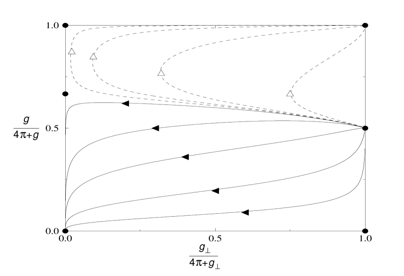
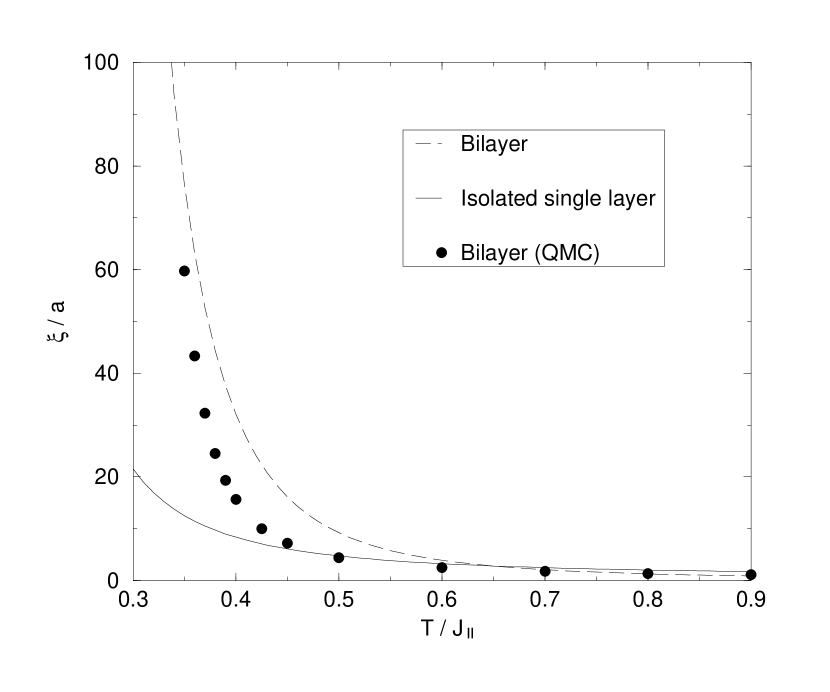
Figure 1: Left: Zero temperature flow diagram.

Figure 2: Right: Correlation lengths of the bilayer antiferromagnet compared to those of the isolated single layer. The solid circles are the Monte Carlo results.

Not unexpectedly there are differences at intermediate temperatures, but the correlation length rapidly approaches Eq. (10) at lower temperatures. We find it surprising that at temperatures as high as $5J_{\perp}(=0.4J_{\parallel})$ the correlation length of the bilayer antiferromagnet is already significantly higher than the correlation length of the single layer antiferromagnet[14].

In summary, the theoretical results obtained here should be important in understanding the magnetic fluctuations of bilayer high temperature superconductors, as they can be explored in neutron scattering experiments using the energy integrated two axis scan. The applicability of this technique is due to the fact that the spin-spin correlation length at low temperatures is exceedingly long in bilayer antiferromagnets[15], and nearly critical fluctuations dominate for the parameter regime that is of experimental interest. The energy integration is thus correctly carried out. The present work shows that the bilayer complex in high temperatures such as YBCO are effectively strongly coupled despite the fact that $J_{\perp}\sim 0.1J_{\parallel}$.

We thank O. Syljuåsen for interesting discussions. This work was supported by the National Science Foundation, Grant. No. DMR-9531575. The QMC calculations were performed on the Hitachi SR2201 massively parallel computer of the computer center at the University of Tokyo.

References

- [1] For a brief review, see \NameChakravarty S. in \BookHigh temperature superconductivity edited \NameBedell K. S. et al. (Addison-Wesley, Redwood City) \Year1990.
- [2] \NameShamoto S. et al. \ReviewPhys. Rev. B \Vol48 \Year1993\Page13817.
- [3] \NameChakravarty S., Halperin B. I., and Nelson D. R. \ReviewPhys. Rev. B \Vol39 \Year1989\Page2344.
- [4] \NameEvertz H. G., Lana G. and Marcu M. \ReviewPhys. Rev. Lett. \Vol70, \Year1993 \Page875; \NameBeard B. B. and Wiese U.-J. \ReviewPhys. Rev. Lett. \Vol77 \Year1996 \Page5130.
- [5] \NameDotsenko A. V. \ReviewPhys. Rev. B \Vol52 \Year1995 \Page9170. There are minor errors in this paper. For large-, is smaller by a factor of 2, and is smaller by a factor of 4.
- [6] \NameChubukov A. V. and Morr D. K. \ReviewPhys. Rev. B \Vol52 \Year1995\Page3521.
- [7] Defining , the renormalization group equation for the angular momentum coupling is given by Since always decreases and its initial value is very small, , it is irrelevant.
- [8] \NameHasenfratz P. and Niedermayer F. \NamePhys. Lett. B \Vol268 \Year1991 \Page231.
- [9] \NameReznik D. et al. \ReviewPhys. Rev. B \Vol54 \Year1996\Page14741; \NameHayden S. M. et al. \NamePhys. Rev. B \Vol54 \Year1996 \Page6905.
- [10] \NameChakravarty S. and Orbach R. \ReviewPhys. Rev. Lett. \Vol64 \Year1990 \Page224.
- [11] \NameImai T. et al. \ReviewPhys. Rev. Lett. \Vol70 \Year1993\Page1002.
- [12] \NameKim J.-K., Landau D.P. and Troyer M. \ReviewPhys. Rev. Lett. \Vol79 \Year1997 \Page1583; \NameBeard B.B., Birgeneau R. J., Greven M. and Wiese U.-J. cond-mat/9709110 Preprint, \Year1997; \NameKim J.-K. and Troyer M. cond-mat/9709333 Preprint, \Year1997; \NameHarada K. , Troyer M. and Kawashima N. cond-mat/9712292 Preprint, \Year1997.
- [13] \NameTyč, S. et al \ReviewPhys. Rev. Lett. \Vol62\Year1989\Page835.
- [14] Numerical simulations were also performed by \NameSandvik A. and Scalapino D. J. \ReviewPhs. Rev. B \Vol53 \Year1996 \PageR526. The present simulations are more accurate and extend to lower temperatures necessary to compare with the analytical results. At higher temperatures where the data can be compared the results are similar.
- [15] The application of the same field theoretical method to -layer antiferromagnet shows that the infinite layer limit is approached exponentially fast, similar to the crossover observed in gapped spin ladders [\NameChakrvarty S. \ReviewPhys. Rev. Lett. \Vol77 \Year1996 \Page4446]—\NameYin L. to be published.