Capacitively coupled Josephson-junction chains: straight and slanted coupling

Abstract

Two chains of ultrasmall Josephson junctions, coupled capacitively with each other in the two different ways, straight and slanted coupling, are considered. As the coupling capacitance increases, regardless of the coupling scheme, the transport of particle-hole pairs in the system is found to drive the quantum-phase transition at zero temperature, which is a insulator-to-superfluid transition of the pairs and belongs to the Berezinskii-Kosterlitz-Thouless universal class. The different underlying transport mechanisms for the two coupling schemes are reflected in the difference between the transition points.

I Introduction

Systems of ultrasmall tunnel junctions composed of metallic or superconducting electrodes have attracted considerable interest owing to the significant roles of the Coulomb interaction in them. First of all, a sufficiently large charging energy leads to the Coulomb blockade effect which exhibits single charge (electron or Cooper pair) tunneling [1]. In order for this tunneling to occur, however, it should be energetically favorable with respect to the electrostatic energy of the system. Otherwise, more complex elementary processes that involve several charge-tunneling events become dominant. In particular, a recent theoretical prediction [2] and an experimental demonstration [3] have revealed the cotunneling of electron-hole pairs in two one-dimensional (1D) metallic tunnel-junction arrays coupled by large inter-array capacitances (see Fig. 1). Such cotunneling of electron-hole pairs results in the remarkable effect of current drag: The current fed through either of the chains induces a secondary current in the other chain. The primary and the secondary currents are comparable in magnitude, but opposite in direction.

A similar current drag effect has also been observed in a slightly different configuration of the system, in which each electrode in one array is coupled aslant to two adjacent electrodes in the other array (slanted coupling; see Fig. 2) [4]. Unlike the case mentioned above (straight coupling; see Fig. 1), where the low-energy state can be preserved only if the electron and the hole tunnel simultaneously (cotunneling), in this case the low-energy state can be preserved for sequential tunneling of the electron and the hole. It has been suggested that this correlated sequential tunneling might be more likely than the second-order process of cotunneling via a quantum-mechanical virtual state.

More interestingly, when the tunneling junctions are composed of ultrasmall superconducting grains, the counter part of the electron-hole pair becomes the pair of an excess and a deficit Cooper pair, which will be simply called a particle-hole pair. Furthermore, in such ultrasmall Josephson-junction systems, the competition between the charging energy and the Josephson coupling energy is well known to bring about the noble effects of quantum fluctuations [5, 6, 7, 8]. In a previous work [9], it was proposed that, combined with these quantum-fluctuation effects, the cotunneling of particle-hole pairs in capacitively coupled 1D Josephson junction arrays (JJAs) drives the insulator-to-superfluid transition of the pairs [9].

In this paper, the previous work [9] on two capacitively coupled 1D JJAs is extended to consider both straight and slanted couplings. The focus will be on the similarities and differences between the two coupling schemes. It is shown that on long-time and long-length scales, the two cases are indistinguishable; as the coupling capacitance increases, both of them exhibits Berezinskii-Kosterlitz-Thouless (BKT)-type insulator-to-superfluid transition, whose superfluid phase is uniquely characterized by the condensation of particle-hole pairs and by perfect drag of supercurrents along the two chains. The correlated tunneling nature of the elementary process in the slanted case is reflected by its lower transition point.

Capacitively coupled JJAs can presumably be realized in experiment, even by current techniques. Recent advances in microfabrication techniques have already made it possible to create large arrays of ultrasmall Josephson junctions [10]. Furthermore, the experimental realization of the capacitively coupled submicron metal-junction arrays [3, 4] illustrates that large interarray capacitances can also be fabricated between two JJAs. In passing, capacitive coupling should be distinguished from Josephson coupling (allowing interarray Cooper-pair tunneling). The quantum-fluctuation effects in the latter case, as in the case of quantum Josephson ladders, have been studied in the literature [11].

The paper is organized as follows: In Section II, the models for the systems with straight or slanted couplings and the regions of interest in parameter space are defined. Section III is devoted to the transformation of the models into equivalent 2D systems of classical vortices. In Section IV, the conductivity of the system is examined in the vortex representation. The results from Sections III and IV provide the bases of this work on which the phase transition and the current-drag effect are discussed in Section V. Section V constitutes the main part of this paper and present a thorough discussion of the role of particle-hole pairs in the quantum-phase transition and the transport in the system. Finally, the paper is concluded in Section VI.

II Models

Each of the two chains ($\ell=1,2$) of Josephson junctions considered here is characterized by the Josephson coupling energy $E_{J}$ and the charging energies $E_{0}{\equiv}e^{2}/2C_{0}$ and $E_{1}{\equiv}e^{2}/2C_{1}$ associated with the self-capacitance $C_{0}$ and the junction capacitance $C_{1}$, respectively (see Fig. 1 and Fig. 2). The two chains are coupled with each other by the capacitance $C_{I}$, with which the electrostatic energy $E_{I}{\equiv}e^{2}/2C_{I}$ is associated. Two different ways of coupling are considered: Each island in one array is coupled one-to-one to one island (straight coupling; Fig. 1) or aslant to two islands (slanted coupling; Fig. 2) in the other array. There is no Cooper-pair tunneling between the chains. The intra-chain capacitances are assumed to be so small ($E_{0},E_{1}\gg{}E_{J}$) that, without the coupling, both chains would each be in the insulating phase [6]. It is also assumed that the coupling capacitance is sufficiently large compared with the intra-array capacitances: $C_{I}\gg{}C_{0},C_{1}$. In that case, the electrostatic energy of the particle-hole pair ($\sim{}E_{I}$) is much smaller than that of an unpaired charge ($\sim{}E_{0},E_{1}$). For the most part, this work is devoted to the case of identical chains, but non-identical chains will also be briefly discussed.

In the specified region of parameter space, the time scale of the relevant dynamics is determined by the coupling capacitance ($C_{I}$) and the corresponding Josephson plasma frequency (${\sim}\sqrt{8E_{I}E_{J}}/\hbar$). To be explicit, for straight coupling, it is convenient to rescale the capacitances by $2C_{I}$ (i.e., $C_{0}/2C_{I}{\to}C_{0},C_{1}/2C_{I}{\to}C_{1}$), the energies by $\hbar\omega_{p}\equiv\sqrt{4E_{I}E_{J}}$, and the times by $1/\omega_{p}$. For slanted coupling, on the other hand, a more convenient choice is a capacitance scale of $4C_{I}$ and a frequency scale of $\hbar\omega_{p}\equiv\sqrt{2E_{I}E_{J}}$. Although it is not essential, throughout this paper, I adopt these normalizations of the physical quantities for simplicity of notation.

Then, the system with straight coupling can be well described by the Hamiltonian (in units of $\hbar\omega_{p}$)

$$H = \frac{1}{2\sqrt{2}K}\sum_{\ell,\ell^{\prime}}\sum_{x,x^{\prime}}n(\ell;x){\mathbb{C}}^{-1}(\ell,\ell^{\prime};x,x^{\prime})n(\ell;x^{\prime})$$ (2)

$$\mbox{}-\sqrt{2}K\sum_{\ell}\sum_{<xx^{\prime}>}\cos\left[\phi(\ell;x)-\phi(\ell;x^{\prime})\right],$$

where the coupling constant has been defined by $K{\equiv}\sqrt{E_{J}/8E_{I}}$. The number $n(\ell;x)$ of excess Cooper pairs and the phase $\phi(\ell;x)$ of the superconducting order parameter on the grain at $x$ in the chain $\ell$ are quantum-mechanically conjugate variables: $[n(\ell;x),\phi(\ell^{\prime};x^{\prime})]{=}i\delta_{xx^{\prime}}\delta_{\ell\ell^{\prime}}$. The Fourier transform of the capacitance matrix in Eq. (2) takes the following form (in units of $2C_{I}$):

$$\widetilde{\mathbb{C}}(q)=\widetilde{C}(q)\left(\begin{array}[]{cc}1&0\\ 0&1\end{array}\right)+\frac{1}{2}\left(\begin{array}[]{rr}1&-1\\ -1&1\end{array}\right),$$ (3)

where $\widetilde{C}(q)\equiv{}C_{0}{+}C_{1}\Delta(q)$, with $\Delta(q)\equiv{}2(1{-}\cos{q})$, is the Fourier transform of the submatrix $C(x,x^{\prime})$ within either of the chains. For slanted coupling, on the other hand, the appropriate Hamiltonian reads as

$$H = \frac{1}{4K}\sum_{\ell,\ell^{\prime}}\sum_{x,x^{\prime}}n(\ell;x){\mathbb{C}}^{-1}(\ell,\ell^{\prime};x,x^{\prime})n(\ell;x^{\prime})$$ (5)

$$\mbox{}-2K\sum_{\ell}\sum_{<xx^{\prime}>}\cos\left[\phi(\ell;x)-\phi(\ell;x^{\prime})\right].$$

In this case, the capacitance matrix (in units of $4C_{I}$) is given by

$$\widetilde{\mathbb{C}}(q) = \widetilde{C}(q)\left(\begin{array}[]{cc}1&0\\ 0&1\end{array}\right)+\frac{1}{4}\left(\begin{array}[]{rr}1&-1\\ -1&1\end{array}\right)$$ (13)

$$\mbox{}+\frac{1}{4}\left(\begin{array}[]{cc}1&-e^{+iq}\\ -e^{-iq}&1\end{array}\right).$$

III 2D Classical Vortex Representations

In this section, I transform each of the models in Eq. (2) and Eq. (5) into equivalent 2D classical system of vortices. The resulting system reveals clearly the nature of the phase transition that will be discussed in Section V.

A Straight Coupling

It is convenient to write the partition function of the system in the imaginary-time path-integral representation as

$$Z=\prod_{\ell,x,\tau}\sum_{n(\ell;x,\tau)}\int_{0}^{2\pi}d\phi(\ell;x,\tau)\;\exp\left[-{\cal S}\right]$$ (14)

with the Euclidean action

$${\cal S} = \frac{1}{2\sqrt{2}K}\sum_{\ell,\ell^{\prime}}\sum_{x,x^{\prime},\tau}n(\ell;x,\tau){\mathbb{C}}^{-1}(\ell,\ell^{\prime};x,x^{\prime})n(\ell;x^{\prime},\tau)$$ (17)

$$\mbox{}-\sqrt{2}K\sum_{\ell}\sum_{x,\tau}\cos\nabla_{x}\phi(\ell;x,\tau)$$

$$\mbox{}+i\sum_{\ell}\sum_{x}n(\ell;x,\tau)\nabla_{\tau}\phi(\ell;x,\tau),$$

where $\nabla_{x}$ and $\nabla_{\tau}$ denote the difference operators with respect to $x$ and $\tau$, respectively, and the (imaginary-)time slice $\delta\tau$ has been chosen to be unity (in units of $1/\omega_{p}$) [12]. The highly symmetric form of Eq. (17) with respect to space and (imaginary) time makes it useful to introduce the space-time 2-vector notation ${\bf r}\equiv(x,\tau)$ and analogous notations for all other vector variables. We then apply the Villain approximation [13] to rewrite the cosine term as summation over an integer field $\{m_{x}(\ell;{\bf r})\}$. Further, with the aid of the Poisson resummation formula [13] and Gaussian integration, we also rewrite the charging energy term as a summation over another integer field $\{m_{\tau}(\ell;{\bf r})\}$ to obtain the partition function

$$Z\sim\prod_{\ell;{\bf r}}\sum_{{\bf m}(\ell;{\bf r})}\int_{-\infty}^{\infty}d\phi(\ell;{\bf r})\;\exp\left\{-{\cal S}\right\}$$ (18)

with

$${\cal S} = \frac{K}{\sqrt{2}}\sum_{\ell,\ell^{\prime};{\bf r},{\bf r}^{\prime}}{\mathbb{C}}(\ell,\ell^{\prime};x,x^{\prime})\delta_{\tau\tau^{\prime}}\;\left[\nabla_{\tau}\phi(\ell;{\bf r})-2\pi m_{\tau}(\ell;{\bf r})\right]\left[\nabla_{\tau}\phi(\ell^{\prime};{\bf r}^{\prime})-2\pi m_{\tau}(\ell^{\prime};{\bf r}^{\prime})\right]$$ (20)

$$\mbox{}+\frac{K}{\sqrt{2}}\sum_{\ell;{\bf r}}\left[\nabla_{x}\phi(\ell;{\bf r})-2\pi m_{x}(\ell;{\bf r})\right]^{2}.$$

The variables $\phi(\ell;{\bf r})$ and ${\bf m}(\ell;{\bf r})$ can be conveniently replaced by $\phi^{\pm}({\bf r})\equiv\phi(1;{\bf r})\pm\phi(2;{\bf r})$ and ${\bf m}^{\pm}({\bf r})\equiv{\bf m}(1;{\bf r})\pm{\bf m}(2;{\bf r})$, respectively. In this way, one decomposes the Euclidean action in Eq. (20) into the sum ${\cal S}={\cal S}^{+}+{\cal S}^{-}$ with ${\cal S}^{\pm}$ defined by

$${\cal S}^{\pm} = +\frac{K}{2\sqrt{2}}\sum_{{\bf r},{\bf r}^{\prime}}C^{\pm}(x,x^{\prime})\delta(\tau,\tau^{\prime})\;\left[\nabla_{\tau}\phi^{\pm}({\bf r})-2\pi m_{\tau}^{\pm}({\bf r})\right]\left[\nabla_{\tau}\phi^{\pm}({\bf r}^{\prime})-2\pi m_{\tau}^{\pm}({\bf r}^{\prime})\right]$$ (22)

$$\mbox{}+\frac{K}{2\sqrt{2}}\sum_{{\bf r}}\left[\nabla_{x}\phi^{\pm}({\bf r})-2\pi m_{x}^{\pm}({\bf r})\right]^{2}.$$

Here, the new capacitance matrices $C^{\pm}(x,x^{\prime})$ have been defined by $\widetilde{C}^{+}(q)=\widetilde{C}(q)$ and $\widetilde{C}^{-}(q)=1+\widetilde{C}(q)$. Now, one follows the standard procedures [14, 6] to integrate out $\{\phi^{\pm}({\bf r})\}$. Apart from the irrelevant spin wave part, one can finally obtain the 2D system of classical vortices, which is also decomposed into two subsystems $H_{V}=H_{V}^{+}+H_{V}^{-}$ with

$$H_{V}^{\pm}=\sqrt{2}\pi^{2}K\sum_{{\bf r},{\bf r}^{\prime}}v^{\pm}({\bf r})\;U^{\pm}({\bf r}-{\bf r}^{\prime})\;v^{\pm}({\bf r}^{\prime}).$$ (23)

where the interactions between vortices are defined via their Fourier transforms

$$\widetilde{U}^{\pm}({\bf q})=\frac{\widetilde{C}^{\pm}(q)}{\Delta(q)+\widetilde{C}^{\pm}(q)\Delta(\omega)}.$$ (24)

It is instructive to notice that the vortices $v^{\pm}$ represent some sorts of correlations between the two chains in the system. In Fig. 3 is represented a configuration of two vortices, $v(1;{\bf r})=+1$ and $v(2;{\bf r}^{\prime})=+1$ (${\bf r}\neq{\bf r}^{\prime}$). This configuration gives a pair of a vortex $v^{-}({\bf r})=+1$ and an antivortex $v^{-}({\bf r}^{\prime})=-1$, which tend to be bound to each other. At the same time, for $v^{+}$, it gives two vortices ($v^{+}({\bf r})=v^{+}({\bf r}^{\prime})=+1$) which are inclined to repel each other. For the configuration with a vortex on one space-time layer and an antivortex on the other, we have opposite tendencies for $v^{+}$ and $v^{-}$. As I will show in Section V, it is the vortices $v^{-}$ that play major roles in the quantum phase transition of the system. Furthermore, the vortices $v^{-}$ will be shown to be manifestations of the particle-hole pairs.

In Eq. (23), $U^{-}(0)$ always diverges and gives rise to the vortex number equality condition $\sum_{\bf r}{}v(1;{\bf r})=\sum_{\bf r}{}v(2;{\bf r})$, or equivalently, the vorticity neutrality condition $\sum_{\bf r}{}v^{-}({\bf r})=0$ for $v^{-}$. A similar neutrality condition, $\sum_{\bf r}{}v^{+}=0$, should be satisfied unless $C_{0}=0$ (see Ref. [8]). More importantly, it should be noticed that the two fields $v^{+}$ and $v^{-}$ actually are not independent of each other since $m_{\mu}(1;{\bf r})$ and $m_{\mu}(2;{\bf r})$ in Eq. (22), and hence $v(1;{\bf r})=[v^{+}({\bf r})+v^{-}({\bf r})]/2$ and $v(2;{\bf r})=[v^{+}({\bf r})-v^{-}({\bf r})]/2$, can take only integer values. As depicted with open circles in Fig. 4, $(v^{+},v^{-})$ at each ${\bf r}$ can take only half of the elements in the product set of integers ${\bf{}Z{\times}Z}$; $v^{+}$ and $v^{-}$ are topologically coupled with each other. However, this topological coupling is irrelevant and can be safely neglected, which will be discussed in more detail in Section V.

B Slanted Coupling

In the same manner as that leading to Eq. (20), from the path-integral representation of the partition function Eq. (14), one can obtain the partition function for slanted coupling:

$$Z\sim\prod_{\ell;{\bf r}}\sum_{{\bf m}(\ell;{\bf r})}\int_{-\infty}^{\infty}d\phi(\ell;{\bf r})\;\exp\left\{-{\cal S}\right\}$$ (25)

with

$${\cal S} = K\sum_{\ell,\ell^{\prime};{\bf r},{\bf r}^{\prime}}{\mathbb{C}}(\ell,\ell^{\prime};x,x^{\prime})\delta_{\tau\tau^{\prime}}\;\left[\nabla_{\tau}\phi(\ell;{\bf r})-2\pi m_{\tau}(\ell;{\bf r})\right]\left[\nabla_{\tau}\phi(\ell^{\prime};{\bf r}^{\prime})-2\pi m_{\tau}(\ell^{\prime};{\bf r}^{\prime})\right]$$ (27)

$$\mbox{}+K\sum_{\ell;{\bf r}}\left[\nabla_{x}\phi(\ell;{\bf r})-2\pi m_{x}(\ell;{\bf r})\right]^{2}.$$

Unlike the previous case, owing to the last term in the capacitance matrix ${\mathbb{C}}$ in Eq. (3), the replacement of the variables $\phi(\ell;{\bf r})$ and ${\bf m}(\ell;{\bf r})$ by $\phi^{\pm}({\bf r})$ and ${\bf m}^{\pm}({\bf r})$, respectively, provides no help at this stage. Instead, we directly integrate out $\phi(\ell;{\bf r})$ to get the Hamiltonian for 2D classical vortices:

$$H_{V} = 4\pi^{2}K\sum_{\ell;{\bf r},{\bf r}^{\prime}}v(\ell;{\bf r})U_{0}({\bf r},{\bf r}^{\prime})v(\ell;{\bf r}^{\prime})$$ (28)

$$+ 4\pi^{2}K\sum_{{\bf r},{\bf r}^{\prime}}v^{-}({\bf r})U_{I}({\bf r},{\bf r}^{\prime})v^{-}({\bf r}^{\prime})$$ (29)

$$+ 4\pi^{2}K\sum_{{\bf r},{\bf r}^{\prime}}v^{-}_{\it sl}({\bf r})U_{I}({\bf r},{\bf r}^{\prime})v^{-}_{\it sl}({\bf r}^{\prime}),$$ (30)

where the vortex interactions are given via the Fourier transforms

$$\widetilde{U}_{0}({\bf q}) = \frac{1}{T({\bf q})}\left[\widetilde{C}(q)\left[\Delta(q)+\left\{1+\widetilde{C}(q)\right\}\Delta(\omega)\right]+\frac{1}{16}\Delta(q)\Delta(\omega)\right],$$ (31)

$$\widetilde{U}_{I}({\bf q}) = \frac{1}{T({\bf q})}\frac{\Delta(q)}{4}$$ (32)

with

$$T({\bf q})=\left[\Delta(q)+\widetilde{C}(q)\Delta(\omega)\right]\left[\Delta(q)+\left\{1+\widetilde{C}(q)\right\}\Delta(\omega)\right]+\frac{1}{16}\Delta(q)\Delta^{2}(\omega).$$ (33)

In Eq. (30), the vortices $v^{-}$ and $v^{-}_{\it{}sl}$ are defined by the direct differences $v^{-}\equiv\left[v(1;{\bf r})-v(2;{\bf r})\right]$ and by the slanted differences $v^{-}_{\it{}sl}\equiv\left[v(1;{\bf r})-v(2;{\bf r}{+}\hat{e}_{x})\right]$ (see Fig. 5). The appearance of the additional term in $v^{-}_{\it{}sl}$ in Eq. (30) is no surprise since with a vortex on one space-time layer the correspondent vortex has two alternative nearest-neighbor sites to sit on on the other space-time layer. However, at the long times and lengths that we are interested in, any configuration of $v^{-}_{\it{}sl}$ gives the same energy as the corresponding configuration of $v^{-}$, which can be seen in Fig. 5. Thus, $v^{-}_{\it{}sl}$ in the last additional term in Eq. (30) can be replaced simply by $v^{-}$, leading to

$$H_{V} \simeq 4\pi^{2}K\sum_{\ell;{\bf r},{\bf r}^{\prime}}v(\ell;{\bf r})U_{0}({\bf r},{\bf r}^{\prime})v(\ell;{\bf r}^{\prime})$$ (34)

$$+ 8\pi^{2}K\sum_{{\bf r},{\bf r}^{\prime}}v^{-}({\bf r})U_{I}({\bf r},{\bf r}^{\prime})v^{-}({\bf r}^{\prime}).$$ (35)

This point can also be seen in a more rigorous way by rewriting the Hamiltonian in Eq. (30) in terms of $v^{\pm}({\bf r})$; i.e., $H_{V}=H_{V}^{+}+H_{V}^{-}+\delta{H}_{V}$, where $H_{V}^{\pm}$ has the anticipated form

$$H_{V}^{\pm}=2\pi^{2}K\sum_{{\bf r},{\bf r}^{\prime}}v^{\pm}({\bf r})\>U^{\pm}({\bf r},{\bf r}^{\prime})\>v^{\pm}({\bf r}^{\prime})$$ (36)

with the vortex interactions

$$\widetilde{U}^{+}({\bf q}) = \frac{1}{T({\bf q})}\left[\widetilde{C}(q)\left[\Delta(q)+\left\{1+\widetilde{C}(q)\right\}\Delta(\omega)\right]+\frac{1}{16}\Delta(q)\Delta(\omega)\right]$$ (37)

$$\widetilde{U}^{-}({\bf q}) = \frac{1}{T({\bf q})}\left[\left\{1+\widetilde{C}(q)\right\}\left\{\Delta(q)+\widetilde{C}(q)\Delta(\omega)\right\}+\frac{1}{16}\Delta(q)\Delta(\omega)\right].$$ (38)

The term $\delta{H}_{V}$, defined by

$$\delta{H}_{V}=\frac{\pi^{2}}{4}K\sum_{\alpha,\beta=\pm}\sum_{{\bf r},{\bf r}^{\prime}}v^{\alpha}({\bf r})\>\delta{U}^{\alpha\beta}\>v^{\beta}({\bf r}^{\prime})$$ (39)

with

$$\delta\tilde{U}^{\alpha\beta}({\bf q})=\frac{\Delta(q)}{T({\bf q})}\left(\begin{array}[]{cc}+\Delta(q)&+2i\sin{q}\\ -2i\sin{q}&-\Delta(q)\end{array}\right),$$ (40)

describes the interaction between $v^{+}$ and $v^{-}$. Since the numerator in the interaction $\delta\widetilde{U}^{\alpha\beta}({\bf q})$ is the third order in ${\bf q}$, at long times and lengths (${\bf q}\to 0$), $\delta{H}_{V}$ can be ignored compared with $H_{V}^{\pm}$. Moreover, in the low frequency and momentum limit (neglecting the terms of order ${\cal{}O}({\bf q}^{4})$ or higher, the vortex interactions in Eqs. (37) and (38) are simply reduced to those in Eq. (24) for straight coupling. For this reason, it is concluded that, at long times and lengths, the 2D vortex representation for slanted coupling is equal to that for straight coupling except for the different coupling constant: $K/\sqrt{2}$ for straight coupling and $K$ for slanted coupling.

IV Linear Response

The mathematical mapping in the previous section enables us to examine the existence and the universal class of the phase transition, and yet we need to identify and characterize the phases on both sides of the transition (see Section V). A common method is to measure the response of the system to an external perturbation. In this section, I consider the conductivity, specifically, the linear response $\sigma_{\ell_{1}\ell_{2}}(\omega)$ of the current in chain $\ell_{1}$ to the voltage applied across chain $\ell_{2}$ (see Fig. 1 and Fig. 2) and rewrite it in the vortex representation in accordance with the previous section.

The response function $\sigma_{\ell_{1}\ell_{2}}(\omega)$ can be obtained via the analytic continuation

$$\sigma_{\ell_{1}\ell_{2}}(\omega)=\frac{1}{i\omega}\lim_{q\to 0}\widetilde{\cal G}_{\ell_{1}\ell_{2}}(q,i\omega^{\prime}\to\omega+i0^{+}),$$ (41)

where $\widetilde{\cal G}_{\ell_{1}\ell_{2}}$ is the Fourier transform of the imaginary-time Green’s function

$${\cal G}_{\ell_{1}\ell_{2}}(x,\tau)=\left\langle T_{\tau}[I(\ell_{1};x,\tau)I(\ell_{2};0,0)]\right\rangle$$ (42)

with the time-ordered product $T_{\tau}$ and the current operators $I(\ell;x)\equiv\sin\nabla_{x}\phi(\ell;x)$. Owing to the symmetry between the two chains, the conductivities $\sigma_{11}$ and $\sigma_{21}$ can be written as

$$\sigma_{11}(\omega) = \frac{1}{4}\left[\sigma_{+}(\omega)+\sigma_{-}(\omega)\right],$$ (43)

$$\sigma_{21}(\omega) = \frac{1}{4}\left[\sigma_{+}(\omega)-\sigma_{-}(\omega)\right]$$ (44)

in terms of $\sigma_{\pm}$ defined in a manner analogous to Eqs. (41) and (42) with $I^{\pm}(x)\equiv{}I(1;x)\pm{}I(2;x)$. In the same manner as in Section II, one can get the vortex representation of the corresponding Green’s functions ${\cal G}_{\pm}$ (see Appendix A):

$${\cal G}_{\pm}({\bf r}_{1},{\bf r}_{2})=\nabla_{\tau_{1}}\nabla_{\tau_{2}}\left\{-\frac{\gamma}{K}U^{\pm}({\bf r}_{1},{\bf r}_{2})+4\pi^{2}\sum_{{\bf r}_{1}^{\prime},{\bf r}_{2}^{\prime}}U^{\pm}({\bf r}_{1},{\bf r}_{1}^{\prime})U^{\pm}({\bf r}_{2},{\bf r}_{2}^{\prime})\left\langle v^{\pm}({\bf r}_{1}^{\prime})v^{\pm}({\bf r}_{2}^{\prime})\right\rangle_{V}\right\},$$ (45)

where $\gamma=\sqrt{2}$ for straight coupling or $\gamma=1$ for slanted coupling, and the average $\left\langle\cdots\right\rangle_{V}$ is with respect to the total vortex Hamiltonian $H_{V}=H_{V}^{+}+H_{V}^{-}$. In Eq. (45), the same Hamiltonians $H_{V}^{\pm}$ as in Eq. (23) and the same interactions $U^{\pm}$ as in Eq. (24) are used both for straight and slanted coupling. This should be valid at the long times and lengths we are interested in, as discussed in the previous section. One of the benefits of the representation in Eq. 45 is that the vortex contribution of the second term in Eq. 45 can be estimated in the standard renormalization group (RG) approach for 2D classical vortices [5, 15].

V Quantum Phase Transitions

Now, I turn to the main subjects of this work, the quantum-phase transition and the current-drag effect in the system based on the 2D classical-vortex representations of the partition functions in Eq. (23) and in Eq. (36) and the response functions in Eq. 41. In Section II, it was established that, aside from the differences in the coupling constant, the two coupling schemes are equivalentat at long times and lengths. First, the discussion will focuse on straight coupling, the results of which can be applied in full to slanted coupling with the coupling constant properly replaced. Some important differences between the two coupling schemes will be discussed at the end of the section.

It is not difficult to understand separately the physics described by each of the Hamiltonians $H_{V}^{\pm}$ in Eq. (23). Unless $C_{0}=0$, the length-dependent anisotropy due to $\widetilde{C}^{+}(q)=\widetilde{C}(q)\ll 1$ in $\widetilde{U}^{+}({\bf q})$ in Eq. (24) fades out on (space-time) length scales larger than $\sqrt{C_{1}/C_{0}}$, and thereby $\widehat{U}^{+}({\bf r})\equiv{}2\pi[U^{+}(0)-U^{+}({\bf r})]$ is simply reduced to the isotropic logarithmic interaction

$$\widehat{U}^{+}({\bf r})\simeq\sqrt{C_{0}}\log{r},\quad(r\gg 1).$$ (46)

This results in the usual vortex Hamiltonian

$$H_{V}^{+}\simeq-\pi K_{\it eff}^{+}\sum_{{\bf r},{\bf r}^{\prime}}v^{+}({\bf r})\log|{\bf r}-{\bf r}^{\prime}|v^{+}({\bf r})$$ (47)

with the effective coupling constant $K_{\it{}eff}^{+}\equiv\sqrt{E_{J}/16E_{0}}$. Because we assumed at the beginning of the paper that $E_{0},E_{1}\gg{}E_{J}$, $K_{\it{}eff}$ is substantially smaller than the BKT transition point $K_{\it{}BKT}\simeq{}2/\pi$; the vortices $v^{+}$ always form a neutral plasma of free vortices regardless of $K$ (i.e., regardless of $C_{I}$). In the case of $C_{0}=0$, $U^{+}({\bf r})$ is only short ranged: $U^{+}({\bf r})\sim\sqrt{C_{1}}\exp(-r/\sqrt{C_{1}})$. In this case, the vortices $v^{+}$ even form a non-neutral plasma of free vortices. In any case, the system of vortices $v^{+}$ always forms a plasma of free vortices, regardless of the value of $K$. On the other hand, neglecting the short-distance anisotropy, $\widehat{U}^{-}({\bf r})$ is isotropic in space-time and logarithmic in distance: $\widetilde{U}^{-}({\bf q})\simeq{}1/[\Delta(q)+\Delta(\omega)]$ and $\widehat{U}({\bf r})\simeq\log{r}$ leading to the 2D Coulomb gas Hamiltonian for $v^{-}$

$$H_{V}^{-}\simeq-\sqrt{2}\pi^{2}K\sum_{{\bf r},{\bf r}^{\prime}}v^{-}({\bf r})\log|{\bf r}-{\bf r}^{\prime}|v^{-}({\bf r}^{\prime}).$$ (48)

It follows that the system of vortices $v^{-}$ exhibits a BKT-type phase transition at $K=K_{c}^{-}$ such that $K_{c}^{-}/\sqrt{2}=K_{\it{}BKT}\simeq{}2/\pi$.

At this point, one might be tempted to conclude that, as $K$ is decreased, the total system $H_{V}$ goes through a BKT-type transition at $\sqrt{2}K_{\it{}BKT}$ which is entirely driven by the vortices $v^{-}$, with $v^{+}$ playing no role. This scenario, however, should be carefully tested against the topological coupling between $v^{+}$ and $v^{-}$ discussed in the previous section.

For this goal, it is convenient to consider the subsystem $\{v^{*}_{\mu}\}$ of $\{v^{+}_{\mu}\}$ satisfying $v^{-}({\bf r})=0$ for all ${\bf r}$. In this subsystem, $v^{*}({\bf r})$ can take only even numbers, and hence the Hamiltonian can be written as

$$H_{V}^{*}\simeq-\pi(4K_{\it{}eff}^{+})\sum_{{\bf r},{\bf r}^{\prime}}[v^{*}({\bf r})/2]\log|{\bf r}-{\bf r}^{\prime}|[v^{*}({\bf r}^{\prime})/2]$$ (49)

unless $C_{0}=0$. Under the assumption $E_{0},E_{1}\gg{}E_{J}$ ($4K_{\it{}eff}^{+}\ll{}K_{\it{}BKT}$), there are a significant number of free vortices of $v^{*}$. Obviously, it is also true in the case of $C_{0}=0$. These free vortices of $v^{*}$ substantially affect the topological coupling and eventually make it irrelevant: As illustrated in Fig. 6, the vortex-antivortex pair of $v^{-}$ is always accompanied by two vortices of $v^{+}$ (enclosed in dotted ellipses). The interaction between these two vortices of $v^{+}$ is completely screened out by the free vortices of $v^{*}$ (indicated by double arrows in the figure). The two vortices of $v^{+}$, therefore, cannot affect the interaction energy of the vortex-antivortex pair of $v^{-}$; they can only slightly change the fugacity of $v^{-}$. It is concluded that, as $K$ is increased, the system exhibits a BKT-type transition at $K_{c}^{\it{}st}\simeq{}\sqrt{2}K_{\it{}BKT}\simeq{}2\sqrt{2}/\pi$, which is exclusively attributed to the vortices $v^{-}$.

To examine the states of the system on both sides of $K_{c}^{\it{}st}$, it is first noted that the vortices $v^{\pm}({\bf r})$ are topological singularities in the 2D space-time configurations of the phases $\phi^{\pm}({\bf r})\equiv\phi(1;{\bf r})\pm\phi(2;{\bf r})$. The plasma of free vortices of $v^{+}$ leads to complete disorder of $\phi^{+}$. Accordingly to the uncertainly relation between $\phi^{+}$ and the conjugate variable $n^{+}(x)\equiv[n(1;x)+n(2;x)]/2$, i.e., $\Delta\phi^{+}\Delta{}n^{+}\geq{}1$, this means that $n^{+}(x)$ for each $x$ takes well-defined value, which should be zero due to the large single-charge(Cooper pair) excitation energy of order of $E_{0}$ or $E_{1}$: $n^{+}(x)=0$. Consequently, the variable $n^{-}(x)\equiv[n(1;x)-n(2;x)]/2$ conjugate to $\phi^{-}$ represents the number of pairs of excess and deficit Cooper pairs (i.e., particle-hole pairs). Further, it is also noted that the effective model in Eq. (23) or Eq. (48) is a vortex representation of the quantum phase model [5, 8]

$$H_{\it QPM}=\frac{1}{\sqrt{2}K}\sum_{x}\left[n^{-}(x)\right]^{2}+\frac{K}{\sqrt{2}}\sum_{x}\cos\nabla_{x}\phi^{-}(x).$$ (50)

Therefore, the BKT-type phase transition at $K_{c}^{\it{}st}$ driven by $v^{-}$ is nothing but an insulator-to-superfluid transition of the particle-hole pairs: Although particle-hole pairs are always the lowest excitations, below $K_{c}^{\it{}st}$, they cannot move along the system without external bias due to the Coulomb blockade associated with the charging energy $E_{I}$. For $K>K_{c}^{\it{}st}$, on the other hand, the particle-hole pairs condensate to form a superfluid and can move free along the system (see Fig. 7). The formation of bound dipoles of vortices $v^{-}$ is an effective manifestation of the condensation of the particle-hole pairs.

Such particle-hole transport can be confirmed by examining the current responses the two chains given by Eq. (41). Due to the free vortices of $v^{+}$, it follows directly from Eq. (45) that $\sigma_{+}(\omega)$ vanishes ($\omega\ll{}1$). On the other hand, the tightly bound vortex-antivortex pairs of $v^{-}$ above $K_{c}^{\it{}st}$ result in the response function

$$\sigma_{-}(\omega)=\frac{2\pi}{\sqrt{2}K}\left(2-\frac{K}{K_{R}}\right)\delta(\omega)\quad(\omega\ll 1),$$ (51)

and hence

$$\sigma_{11}(\omega)=-\sigma_{21}(\omega)=\frac{\pi}{2\sqrt{2}K}\left(2-\frac{K}{K_{R}}\right)\delta(\omega),$$ (52)

where the renormalized coupling constant $K_{R}$ is defined by

$$\frac{\sqrt{2}}{K_{R}}\equiv\frac{\sqrt{2}}{K}-\frac{\pi^{2}}{2}\sum_{\bf r}|{\bf r}|^{2}\left\langle v^{-}({\bf r})v^{-}({\bf 0})\right\rangle.$$ (53)

Thus the system exhibits superconductivity and carries currents along the two chains equally large in magnitude but opposite in direction. This perfect drag of supercurrents reveals that the charges indeed transport in the form of particle-hole pairs, which are bound by the electrostatic energy $E_{I}$ associated with $C_{I}$. For $K<K_{c}^{\it{}st}$, on the other hand, the system displays insulating particle-hole $I$-$V$ characteristics, qualitatively the same as those in Refs. [2, 3, 4].

The argument so far also holds for slanted coupling if only one replaces $K/\sqrt{2}$ by $K$; the system with slanted coupling exhibits a BKT-type transition at $K_{c}^{\it{}sl}\simeq{}K_{\it{}BKT}$, and the superfluid state is characterized by the response functions

$$\sigma_{11}(\omega)=-\sigma_{21}(\omega)=\frac{\pi}{4K}\left(2-\frac{K}{K_{R}}\right)\delta(\omega),$$ (54)

where

$$\frac{1}{K_{R}}\equiv\frac{1}{K}-\frac{\pi^{2}}{2}\sum_{\bf r}|{\bf r}|^{2}\left\langle v^{-}({\bf r})v^{-}({\bf 0})\right\rangle.$$ (55)

It is interesting, however, to notice that $K_{c}^{\it{}sl}$ is quite a bit smaller than $K_{c}^{\it{}st}$ (see Fig. 7). This reflects the difference between the two coupling scheme in the underlying transport mechanism: The correlated sequential tunneling of particle-hole pairs, a first-order process, is more likely than cotunneling, a second-order process.

VI Conclusion

In conclusion, the properties associated with particle-hole pairs in two capacitively coupled Josephson-junction chains, considering both the straight and the slanted couplings have been investigated. In particular, the transport of particle-hole pairs was found to drive the BKT-type insulator-to-superfluid transition with respect to the coupling capacitance, regardless of the coupling scheme. The superfluid phase ($K>K_{c}$) is uniquely characterized by the absolute drag of supercurrents along the two chains.

A

In this appendix, the vortex-representation of the imaginary-time Green’s function in Eq. (45) is derived. For simplicity, only the ${\cal G}_{-}$ for straight coupling is derived here. The application of the same approach to ${\cal G}_{+}$ should be straightforward, though. In addition, at long times and lengths, the derivation should also hold for slanted coupling if one replace $K/\sqrt{2}$ by $K$ (see Section III).

In the imaginary-time path-integral representation, the Green’s function ${\cal G}_{-}({\bf r}_{1},{\bf r}_{2})\equiv\left\langle{I_{-}({\bf r}_{1})I_{-}({\bf r}_{2})}\right\rangle$ can be written as

$${\cal G}_{-}({\bf r}_{1},{\bf r}_{2}) = \frac{1}{2K^{2}Z}\prod_{\ell;{\bf r}}\sum_{n(\ell;{\bf r})}\int_{0}^{2\pi}d\phi(\ell;{\bf r})\;\left\{\frac{\partial}{\partial\nabla_{x}\phi(1;{\bf r}_{1})}-\frac{\partial}{\partial\nabla_{x}\phi(2;{\bf r}_{1})}\right\}$$ (A2)

$$\mbox{}\times\left\{\frac{\partial}{\partial\nabla_{x}\phi(1;{\bf r}_{2})}-\frac{\partial}{\partial\nabla_{x}\phi(2;{\bf r}_{2})}\right\}\exp\left\{-{\cal S}[n,\phi]\right\},$$

where the Euclidean action ${\cal S}$ is given by Eq. (17). By changing the variables from $\phi(\ell;{\bf r})$ and ${\bf m}(\ell;{\bf r})$ to $\phi^{\pm}({\bf r})$ and ${\bf m}^{\pm}({\bf r})$, respectively, one obtains

$${\cal G}_{-}({\bf r}_{1},{\bf r}_{2})=\frac{2}{K^{2}Z}\prod_{\alpha=\pm}\prod_{\bf r}\sum_{{\bf m}^{\alpha}({\bf r})}\int d\phi^{\alpha}({\bf r})\;\frac{\partial}{\partial\nabla_{x}\phi^{-}({\bf r}_{1})}\frac{\partial}{\partial\nabla_{x}\phi^{-}({\bf r}_{2})}\exp\left\{-{\cal S}^{+}-{\cal S}^{-}\right\}.$$ (A3)

${\cal S}^{\pm}$ has been given in Eq. (22). The $\phi^{\pm}$-integration can be performed easier by first introducing an auxiliary field as follows:

$${\cal G}_{-}({\bf r}_{1},{\bf r}_{2})=-\frac{2}{K^{2}Z}\prod_{\alpha;{\bf r}}\sum_{{\bf m}^{\alpha}({\bf r})}\int d\phi^{\alpha}({\bf r})\int d^{2}{\bf J}^{\alpha}({\bf r})\;J^{-}_{x}({\bf r}_{1})J^{-}_{x}({\bf r}_{2})\exp\left\{-{\cal S}^{+}-{\cal S}^{-}\right\},$$ (A4)

where

$${\cal S}^{\pm} = \frac{1}{\sqrt{2}K}\sum_{{\bf r},{\bf r}^{\prime}}J_{\tau}^{\pm}({\bf r})\>\left[C^{\pm}({\bf r},{\bf r}^{\prime})\right]^{-1}J_{\tau}^{\pm}({\bf r}^{\prime})+\frac{1}{\sqrt{2}K}\sum_{{\bf r},{\bf r}^{\prime}}\left[J_{x}^{\pm}({\bf r})\right]^{2}$$ (A6)

$$\mbox{}+i\sum_{\bf r}{\bf J}({\bf r})\cdot\left[\nabla\phi^{\pm}({\bf r})-2\pi{\bf m}^{\pm}({\bf r})\right].$$

Now, integrating out $\phi^{\pm}({\bf r})$, one finally gets the vortex-representation of the Green’s function ${\cal G}_{-}$:

$${\cal G}_{-}({\bf r}_{1},{\bf r}_{2})=\nabla_{\tau_{1}}\nabla_{\tau_{2}}\left\{-\frac{\sqrt{2}}{K}U^{-}({\bf r}_{1},{\bf r}_{2})+4\pi^{2}\sum_{{\bf r}_{1}^{\prime},{\bf r}_{2}^{\prime}}U^{-}({\bf r}_{1},{\bf r}_{1}^{\prime})U^{-}({\bf r}_{2},{\bf r}_{2}^{\prime})\left\langle v^{-}({\bf r}_{1}^{\prime})v^{-}({\bf r}_{2}^{\prime})\right\rangle_{V}\right\},$$ (A7)

where the average $\left\langle\cdots\right\rangle_{V}$ is with respect to the total vortex Hamiltonian $H_{V}=H_{V}^{+}+H_{V}^{-}$.

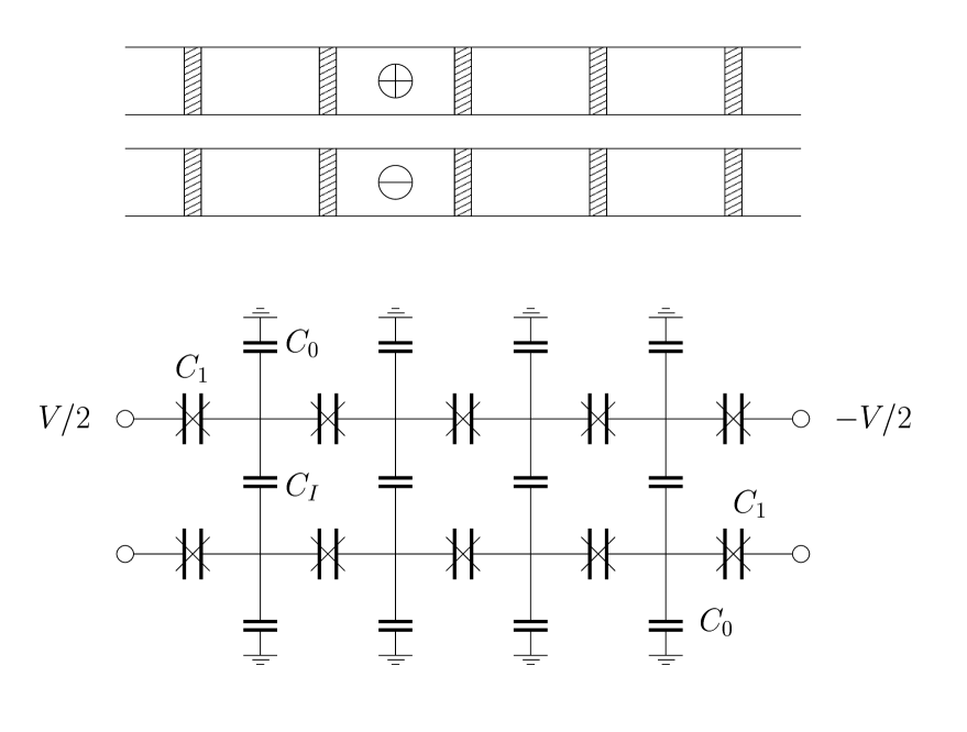
FIG. 1.: Schematic picture and equivalent circuit of the system with straight inter-chain coupling. After Averin, Korotkov, and Nazarov, Phys. Rev. Lett. 66, 2818 (1991).

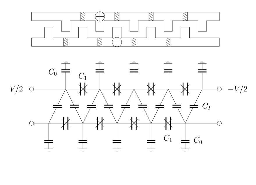
FIG. 2.: Schematic picture and equivalent circuit of the system with slanted inter-chain coupling. After Delsing, Haviland, and Davidsson, Czech. J. Phys. 46, 2359 (1996).

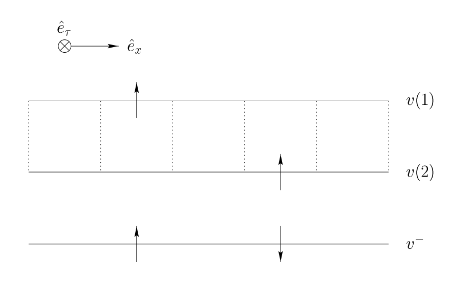
FIG. 3.: Displacement vortex $v^{-}$. The configuration of one vortex $v(1;{\bf r}){=}{+}1$ on space-time layer $1$ and another $v(2;{\bf r}^{\prime}){=}{+}1$ on layer $2$ (${\bf r}\neq{\bf r}^{\prime}$) corresponds to a pair of displacement vortices, a vortex $v^{-}({\bf r}){=}{+}1$ and an antivortex $v^{-}({\bf r}^{\prime}){=}{-}1$.

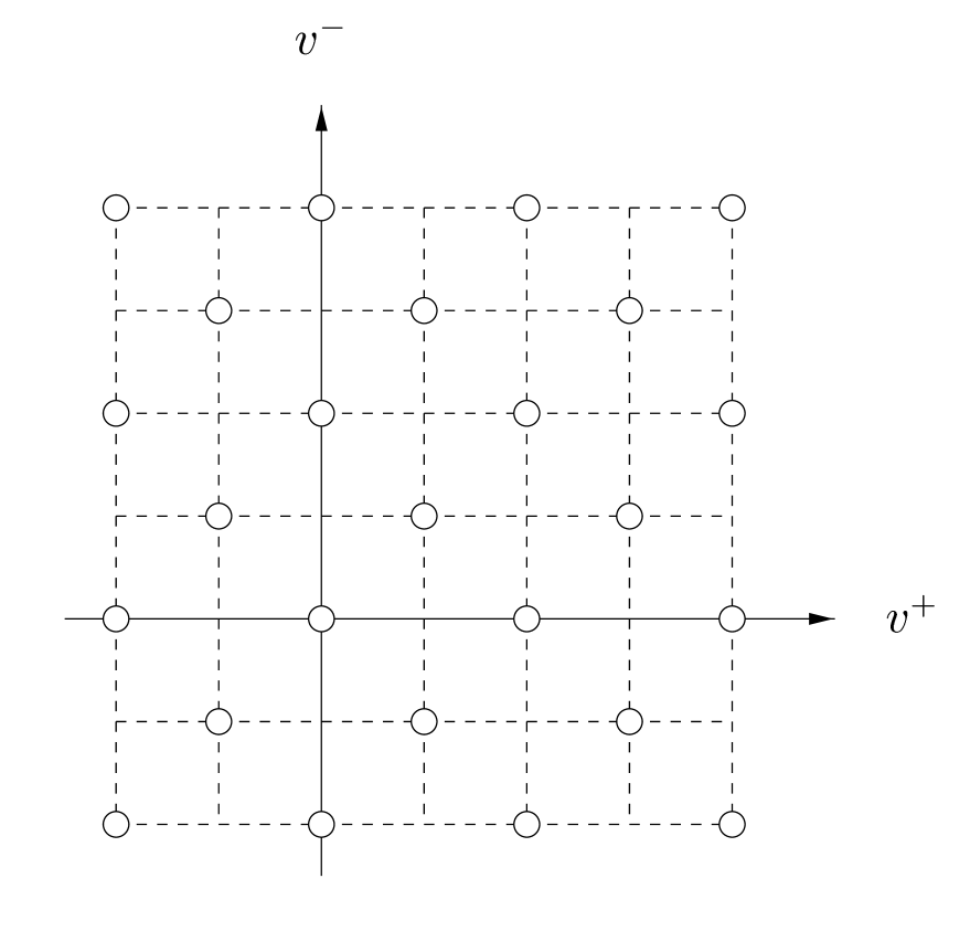
FIG. 4.: Topological coupling of $v^{+}$ and $v^{-}$. At each space-time position $\vec{\bf r}$, $(v^{+},v^{-})$ can take only half of the elements in ${\bf{}Z{\times}Z}$ as depicted with the open circles in the figure.

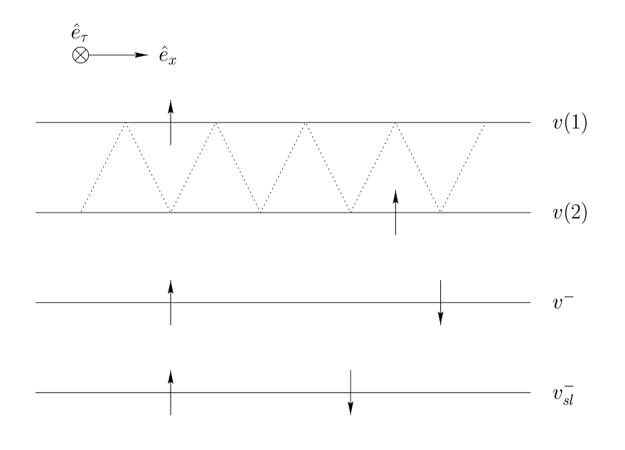
FIG. 5.: Displacement vortex for slanted coupling. At long (space-time) lengths, the vortex-antivortex pair of $v^{-}_{\it{}sl}$ gives the same energy as that of $v^{-}$.

FIG. 6.: Due to the topological coupling, the vortex-antivortex pair of the displacement vortices $v^{-}$ (indicated by dotted ellipses) induces two vortices of $v^{+}$. The interaction between these two vortices is, however, completely screened out by the free vortices of $v^{+}$ with $\pm 2$ (indicated by the douple arrows).

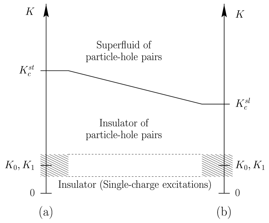
FIG. 7.: Phase diagrams of capacitively coupled Josephson-junction chains (a) with straight coupling and (b) with slanted coupling. The intra-chain coupling constants $K_{0}$ and $K_{1}$ are defined by $K_{0}\equiv\sqrt{E_{J}/8E_{0}}\propto\sqrt{C_{0}}$ and by $K_{1}\equiv\sqrt{E_{J}/8E_{1}}\propto\sqrt{C_{1}}$, respectively. In the text, only the region of $K\gg{}K_{0},K_{1}$, where particle-hole pairs are relevant, is considered.

REFERENCES

• [1] Single Charge Tunneling: Coulomb Blockade Phenomena in Nanostructures, edited by H. Grabert and M. Devoret (Plenum Press, New York, 1992); D. V. Averin and K. K. Likharev, in Mesoscopic Phenomena in Solids, edited by B. L. Al’tshuler, P. A. Lee, and R. A. Webb (Elsvier Science, Amsterdam, 1991), p. 167; G. Schön, and A. D. Zaikin, Phys. Rep. 198, 237 (1990).
• [2] D. V. Averin, A. N. Korotkov, and Y. V. Nazarov, Phys. Rev. Lett. 66, 2818 (1991).
• [3] M. Matters, J. J. Versluys, and J. E. Mooij, Phys. Rev. Lett. 78, 2469 (1997).
• [4] P. Delsing, D. B. Haviland, and P. Davidsson, Czech. J. Phys. 46, 2359 (1996).
• [5] R. M. Bradley and S. Doniach, Phys. Rev. B 30, 1138 (1984).
• [6] R. Fazio and G. Schön, Phys. Rev. B 43, 5307 (1991); A. van Otterlo, K.-H. Wagenblast, R. Fazio, and G. Schön, ibid. 48, 3316 (1993).
• [7] B. J. Kim and M. Y. Choi, Phys. Rev. B 52 (5), 3624 (1995); ibid. 56, 395 (1997).
• [8] M.-S. Choi et al., Phys. Rev. B 57, R716 (1998).
• [9] M.-S. Choi, M. Y. Choi, and S.-I. Lee, preprint (submitted to Phys. Rev. Lett.).
• [10] See, e.g., G. Schön, and A. D. Zaikin, Phys. Rep. 198, 237 (1990), and references therein.
• [11] See, e.g., E. Granato, Phys. Rev. B 42, 4797 (1990); ibid. 45, 2557 (1992); ibid. 48, 7727 (1993).
• [12] The critical behavior of the system should not be affected by the choice of $\delta\tau$. See, e.g., S. L. Sondhi, S. M. Girvin, J. P. Carini and D. Shahar, Rev. Mod. Phys. 69, 315 (1997). Here, all the dynamics of the system occurs over the time scale $\omega_{p}^{-1}$, making it proper to choose $\delta\tau\sim\omega_{p}^{-1}$.
• [13] J. V. José, L. P. Kadanoff, S. Kirkpatrick, and D. R. Nelson, Phys. Rev. B 16, 1217 (1977).
• [14] S. E. Korshunov, Europhys. Lett. 11, 757 (1990).
• [15] J. M. Kosterlitz, J. Phys. C 7, 1047 (1974).
Refer to caption