Phase Separation and Coarsening in One-Dimensional Driven Diffusive Systems: Local Dynamics Leading to Long-Range Hamiltonians

Abstract

A driven system of three species of particle diffusing on a ring is studied in detail. The dynamics is local and conserves the three densities. A simple argument suggesting that the model should phase separate and break the translational symmetry is given. We show that for the special case where the three densities are equal the model obeys detailed balance and the steady-state distribution is governed by a Hamiltonian with asymmetric long-range interactions. This provides an explicit demonstration of a simple mechanism for breaking of ergodicity in one dimension. The steady state of finite-size systems is studied using a generalized matrix product ansatz. The coarsening process leading to phase separation is studied numerically and in a mean-field model. The system exhibits slow dynamics due to trapping in metastable states whose number is exponentially large in the system size. The typical domain size is shown to grow logarithmically in time. Generalizations to a larger number of species are discussed.

I Introduction

Collective phenomena in systems far from thermal equilibrium have been of considerable interest in recent years [1]. Unlike systems in thermal equilibrium where the Gibbs picture provides a theoretical framework within which such phenomena can be studied, here no such framework exists and one has to resort to studies of specific models in order to gain some understanding of the phenomena involved.

One class of such models is driven diffusive systems (DDS) [2, 3]. Driven by an external field these systems do not generically obey detailed balance so that the steady state has non-vanishing currents. Theoretical studies of DDS have revealed basic differences between systems in thermal equilibrium and systems far from thermal equilibrium. For example, it is well known that one dimensional ($1d$) systems in thermal equilibrium with short-range interactions do not exhibit phenomena such as phase transitions, spontaneous symmetry breaking (SSB) and phase separation (except in the limit of zero temperature or in the context of long-range interactions) [4]. In contrast, some examples of noisy $1d$ DDS with local dynamics have been found to exhibit such phenomena.

One example of a noisy system which exhibits SSB in $1d$ is the asymmetric exclusion model of two types of charge studied in [5, 6]. In this model, two types of charge are biased to move in opposite directions on a $1d$ lattice with open ends. The charges interact via a hard-core interaction, and are injected at one end of the lattice and ejected at the other end. This model is symmetric under the combined operations of charge conjugation and parity (PC symmetry). However, this symmetry is broken in the steady state, where the currents of the two charges are not equal. The reason for symmetry breaking in this model lies to some extent in the open boundaries. Other examples of models in which there is SSB in $1d$ have also been found in the context of cellular automata [7] and surface growth [8, 9]. In the latter, SSB was due to the fact that one of the rates for a local dynamical move in the models is zero. Once this zero rate changes to a non-zero rate SSB disappears.

A closely related problem to spontaneous symmetry breaking, is that of phase separation in $1d$ noisy systems. This has been observed in driven diffusive models with inhomogeneities, such as defect sites [10] or particles [11]. In these models it has been found that macroscopic regions of high densities are formed near the defect, much like a high density of cars behind a slow car in a traffic jam [12, 13]. Here the phase separation is triggered by the defects. It is of interest to study whether phase separation can occur in $1d$ noisy homogeneous systems such as on a ring geometry with no defects, where all possible local transition rates which are consistent with the symmetry and conservation laws of the model are non vanishing. Recently, Lahiri and Ramaswamy have introduced a lattice model in the context of sedimenting colloidal crystals, where phase separation is found to take place without any inhomogeneities [14]. In this model, there are two rings coupled to each other and particles on each ring undergo an asymmetric exclusion process. The hopping rate between sites $i$ and $i+1$ on each ring depends on the occupation at the $i$th site on the other ring. However, this model is studied mainly using Monte Carlo simulations and no analytical results are available so far.

In a recent Letter [15] we introduced a simple three-species driven diffusive model exhibiting phase separation and spontaneous breaking of the translational symmetry on a ring. In the model nearest-neighbor particles exchange with given rates and the numbers of each species are conserved under the dynamics. The rates of all local dynamical moves that obey the conservation laws are non zero. An argument indicating that generically the system phase separates, thus breaking the translational invariance, was given for the case when none of the species of particle has zero density. In the special case of equal number of particles of each type, it was shown that the local dynamics obeys detailed balance with respect to a long-range asymmetric (chiral) Hamiltonian. In this special case, using the Hamiltonian, we have found the steady state of the model exactly and have been able to prove the existence of phase separation analytically.

The existence of a Hamiltonian for this special case is of interest in the light of speculation that non-equilibrium systems exhibiting generic long-range correlations might be described by effective Hamiltonians containing long-range interactions [16, 17]. Here we explicitly demonstrate that for the special case where the three densities are equal the model is exactly described by a long-range asymmetric Hamiltonian. The model not only has long-range correlations but has generic long-range order. The mechanism found in this study suggests that systems with dynamical rules defined completely locally and a priori without respect to any Hamiltonian, may have a steady state where the configuration space is sampled according to a measure that is intrinsically global. The Hamiltonian also allows us to identify the analog of a temperature in the microscopic dynamics as related to the drive of the system; for zero drive, that is symmetric diffusion of the particles, the effective temperature is infinite and phase separation is lost.

We note that a related but distinct three-species model has recently been introduced by Arndt et al. This model also exhibits phase separation[18].

In the present work we analyze in detail the $M=3$ species model which was introduced in [15] and then generalize it to larger $M$. We provide the complete proof of phase separation which follows from the exact calculation of the partition sum in the thermodynamic limit. We also provide numerical evidence of phase separation in the general case where the densities of the three particles are not equal.

In order to study the coarsening process Monte-Carlo simulations are performed. However, simulation of the microscopic model is hampered by slow dynamics which makes it difficult to access the scaling regime. The system becomes trapped in metastable states comprising several domains of each type of particle. The number of metastable states is exponentially large in the system size. The lifetimes of the metastable states increase exponentially with the average domain size as the fully phase separated state is approached. Thus the model provides an example of slow dynamics in a system without any quenched disorder [19].

To ameliorate the difficulty of numerically studying such slow dynamics we employ a toy model wherein it is the domains that are updated rather than the individual particles. This allows the long-time scaling behavior of the domain size to be investigated and to confirm a logarithmic growth of the average domain size with time. The toy model also affords a mean-field solution for the long-time dynamical behavior, that again confirms the scaling behavior.

Returning to the case of equal numbers of particles of different species it is of interest to investigate the steady-state behavior in finite-size systems. We have found it convenient to do this by employing a matrix product technique previously used to solve the steady state of asymmetric exclusion processes [20]. However, in the case of three species the simplest form of this technique [11, 20, 12] is applicable only to a limited class of systems [21]. For the present model we generalize the matrix product to a product of rank 6 tensors and write the steady state by taking an appropriate contraction. The partition sum and steady-state correlation functions can be conveniently computed numerically using this tensor product ansatz.

The paper is organized as follows: in section II we define the model introduced in [15] and we present an argument which indicates that the system should phase separate as long as none of the species of particles has zero density. In section III we study the special case where the model satisfies detailed balance and explicitly write down the steady-state weight for the three-species model. The existence of phase separation in the model for any non-infinite temperature is proved analytically by calculating some bounds on the two-point correlation functions. Section IV contains numerical evidence for phase separation in the general case where the densities of the three species of particles are not equal. The toy model, which facilitates efficient Monte Carlo simulations, is used to study the dynamics of phase separation. A mean-field analysis of this toy model is presented, the details being left to Appendix A. In Section V we present results for finite systems obtained via the tensor product ansatz. Using these results we study finite-size scaling in the system. In section VI we address phase separation in systems with more than three species of particle and a proof of detailed balance for special cases is given in Appendix B. We conclude in section VII and discuss some open questions.

II Definition of the model

We start by defining a three-species model which exhibits phase separation in $1d$. Consider a one-dimensional, ring-like (periodic) lattice of length $N$ where each site is occupied by one of the three types of particles, $A$, $B$, or $C$. The model evolves under a random sequential update procedure which is defined as follows: at each time step two neighboring sites are chosen randomly and the particles at these sites are exchanged according to the following rates

(1)

The particles thus diffuse asymmetrically around the ring. The dynamics conserves the number of particles, $N_{A},N_{B}$ and $N_{C}$ of the three species.

The $q=1$ case is special. Here the diffusion is symmetric and every local exchange of particles takes place with the same rate as the reverse move. The system thus obeys detailed balance reaching a steady state in which all microscopic configurations (compatible with the number of particles $N_{A},N_{B}$ and $N_{C}$) are equally probable. This state is homogeneous, and no phase separation takes place. We now present a simple argument suggesting that for $q\neq 1$ the steady state of the system is not homogeneous in the thermodynamic limit. For simplicity the case $q<1$ is examined. As a result of the bias in the exchange rates an $A$ particle prefers to move to the left inside a $B$ domain and to the right inside a $C$ domain. Similarly the motion of $B$ and $C$ particles in foreign domains is biased. Consider the dynamics starting from a random initial configuration. The configuration is composed of a random sequence of domains of $A$, $B$, and $C$ particles. Due to the bias a local configuration in which an $A$ domain is placed to the right of a $B$ domain is unstable and the two domains exchange places on a relatively short time scale which is linear in the domain size. Similarly, $AC$ and $CB$ domains are unstable too. On the other hand $AB$, $BC$ and $CA$ configurations are stable and long lived. Thus after a relatively short time the system reaches a state of the type $\ldots AAABBCCAABBBCCC\ldots$ in which $A,B$ and $C$ domains are located to the right of $C,A$ and $B$ domains, respectively. The evolution of this state takes place via a slow diffusion process in which, for example, the time scale for an $A$ particle to cross an adjacent $B$ domain is $q^{-l}$, where $l$ is the size of the $B$ domain. The system therefore coarsens and the average domain size increases with time as $\ln t/|\ln q|$ [22]. Eventually the system phase separates into three domains of the three species of the form $A\ldots AB\ldots BC\ldots C$.

In a finite system the phase separated state may further evolve and become disordered due to fluctuations. However, the time scale for this to happen grows exponentially with the system size. For example it would take a time of order of $q^{-min\{N_{B},N_{C}\}}$ for the $A$ domain in the totally phase separated state to break up into smaller domains. Hence in the thermodynamic limit, this time scale diverges and the phase separated state remains stable provided the density of each species is non-zero. Note that there are always small fluctuations about a totally phase separated state. However, these fluctuations affect the densities only near the domain boundaries. They result in a finite width for the domain walls. The fact that any phase separated state is stable for a time exponentially long in the system size amounts to a breaking of the translational symmetry.

Since the exchange rates are asymmetric, the system generically supports a particle current in the steady state. To see this, consider the $A$ domain in the phase separated state. An $A$ particle near the $\ldots AB\ldots$ boundary can traverse the entire $B$ domain to the right with an effective rate proportional to $q^{N_{B}}$. Once it crosses the $B$ domain it will move through the $C$ domain with rate $1-q$. Similarly an $A$ particle near the $\ldots CA\ldots$ boundary can traverse the entire $C$ domain to the left with a rate proportional to $q^{N_{C}}$. Once the domain is crossed it moves through the $B$ domain with rate $1-q$. Hence the net $A$ particle current is of the order of $q^{N_{B}}-q^{N_{C}}$. Since this current is exponentially small in system size, it vanishes in the thermodynamic limit. For the case of $N_{A}=N_{B}=N_{C}$, this argument suggests that the current is strictly zero for any $N$. In sections III and V we study this case in detail.

The arguments presented above suggesting phase separation for $q<1$ may be easily extended to $q>1$. In this case, however, the phase separated state is $BAC$ rather than $ABC$. This may be seen by noting that the dynamical rules are invariant under the transformation $q\rightarrow 1/q$ together with $A\leftrightarrow B$.

III Special Case $N_{A}=N_{B}=N_{C}$

In this section we show that the dynamics (1), for the special case $N_{A}=N_{B}=N_{C}$, satisfies detailed balance. The corresponding Hamiltonian, which determines the steady-state distribution, is found to have long-range asymmetric interactions. Using this Hamiltonian, we calculate analytically the partition sum and bounds on the correlation functions in the thermodynamic limit. These are then used to prove the existence of phase separation in the model. Later, in section V we study finite systems for this case and the approach to the thermodynamic limit.

A Detailed Balance

The general argument presented in the previous section suggests that for the special case $N_{A}=N_{B}=N_{C}$, the steady state carries no current for any system size. We demonstrate this explicitly by showing that the local dynamics of the model satisfies detailed balance with respect to a long-range asymmetric Hamiltonian ${\cal H}$.

We define the occupation variables $A_{i},B_{i}$ and $C_{i}$ as follows:

$$A_{i}=\left\{\begin{array}[]{ll}1&\text{if site $i$ is occupied by an $A$ particle}\\ 0&\text{otherwise. }\end{array}\right.$$ (4)

The variables $B_{i}$ and $C_{i}$ are defined similarly. Clearly the relation $A_{i}+B_{i}+C_{i}=1$ is satisfied. A microscopic configuration is thus described by a set $\{X_{i}\}=\{A_{i},B_{i},C_{i}\}$. Using these variables, we will show that the Hamiltonian ${\cal H}$ and the steady-state distribution $W_{N}$ corresponding to the dynamics (1) for the case $N_{A}=N_{B}=N_{C}=N/3$ are given by

$${\cal H}(\{X_{i}\})=\sum_{i=1}^{N-1}\sum_{j=i+1}^{N}[C_{i}B_{j}-C_{i}A_{j}+B_{i}A_{j}]\;,$$ (5)

$$W_{N}(\{X_{i}\})=Z_{N}^{-1}q^{{\cal H}(\{X_{i}\})}\;.$$ (6)

Here $Z_{N}$ is the partition sum given by $\sum q^{{\cal H}(\{X_{i}\})}$, where the sum is over all configurations in which $N_{A}=N_{B}=N_{C}$. Note that the Hamiltonian ${\cal H}$ does not determine the dynamics of the system, it just governs the steady-state distribution as given in (5) and (6). Eq. (6) suggests that $q$ serves as a temperature variable with $kT=-1/\ln q$. Thus, $q\to 1$ is the infinite-temperature limit. The Hamiltonian (5) is written in a form which is not manifestly translationally invariant. However, careful examination reveals that when the relation $N_{A}=N_{B}=N_{C}$ is taken into account, the Hamiltonian as given by (5) is indeed translationally invariant (see Appendix B). Therefore site $1$ may be chosen arbitrarily. An expression for ${\cal H}$ which is manifestly translationally invariant will be derived at the end of this section.

Note that

$$\sum_{i=1}^{N-1}\sum_{j=i+1}^{N}(C_{i}A_{j}+A_{i}C_{j})=(N/3)^{2}$$ (7)

since the LHS yields the number of $CA$ (and $AC$) pairs in the system. Using this relation the Hamiltonian may also be written in a form where the cyclic symmetry is more apparent:

$${\cal H}(\{X_{i}\})=\sum_{i=1}^{N-1}\sum_{j=i+1}^{N}[C_{i}B_{j}+A_{i}C_{j}+B_{i}A_{j}]-(N/3)^{2}\;.$$ (8)

The proof of Eqs. (5,6) is straightforward. This is done by considering a nearest-neighbor particle exchange and verifying that detailed balance is satisfied with respect to (6). We start by considering nearest-neighbor sites in the interior of the lattice, namely pairs other than $(1,N)$. For example consider the exchange $AB\rightarrow BA$ taking place at two adjacent sites $k$ and $k+1$, where $k\neq N$. This exchange results in the contribution of one more $B_{i}A_{j}$ term in $\cal H$ and hence the energy of the resulting configuration is higher by $1$. It is easy to see using Eq. (6) that $qW_{N}(\ldots AB\ldots)=W_{N}(\ldots BA\ldots)$, as required by detailed balance. Similar relations are easily derived for exchange of $BC$ and $CA$ pairs. Now consider an exchange taking place between sites $N$ and $1$, say $CA\rightarrow AC$. According to (5) this exchange costs an energy of $2N_{B}-N_{A}-N_{C}+1$. Therefore the exchange satisfies the detailed balance condition $qW_{N}(A\ldots C)=W_{N}(C\ldots A)$ only when $2N_{B}=N_{A}+N_{C}$. Similarly, by considering the exchanges $AB\rightarrow BA$ and $BC\rightarrow CB$, one deduces that the detailed balance condition is satisfied for any exchange at sites $N$ and $1$ as long as $N_{A}=N_{B}=N_{C}$. In Appendix B we consider the most general nearest-neighbor exchange rates for $M$ species and arbitrary densities and derive conditions (B7) for exchange rates which satisfy detailed balance.

To write ${\cal H}$ in a manifestly translationally invariant form we define ${\cal H}_{i_{0}}(\{X_{i}\})$ as the Hamiltonian in which site $i_{0}$ is the origin. Namely,

$${\cal H}_{i_{0}}(\{X_{i}\})=\sum_{i=i_{0}}^{N+i_{0}-2}\sum_{j=i+1}^{N+i_{0}-1}[C_{i}B_{j}-C_{i}A_{j}+B_{i}A_{j}]\;,$$ (9)

where the summation over $i$ and $j$ is modulo $N$. Summing (9) over all $i_{0}$ and dividing by $N$, one obtains,

$${\cal H}(\{X_{i}\}) = \sum_{i=1}^{N}\sum_{k=1}^{N-1}(1-\frac{k}{N})(C_{i}B_{i+k}-C_{i}A_{i+k}+B_{i}A_{i+k})$$ (10)

$$= \sum_{i=1}^{N}\sum_{k=1}^{N-1}(1-\frac{k}{N})(C_{i}B_{i+k}+A_{i}C_{i+k}+B_{i}A_{i+k})-(N/3)^{2}\;,$$ (11)

where in the summation the value of the site index $(i+k)$ is modulo $N$. In the Hamiltonian (10) the interaction is linear in the distance between the particles, and thus is long-ranged. The distance is measured in a preferred direction from site $i$ to site $i+k$. Moreover it is asymmetric in the sense that $\cal H$ is not invariant under the parity operation. It is also related to chiral Hamiltonians [23].

B Ground States and Metastable States

Before proceeding further to evaluate the partition sum and some correlation functions associated with the Hamiltonian (5) let us make a few observations. The ground state of the Hamiltonian is given by the fully separated state $A\ldots AB\ldots BC\ldots C$ and its translationally related states. The degeneracy of the ground state is thus $N$ and its energy is zero. A simple way of evaluating the energy of an arbitrary configuration is obtained by noting that nearest-neighbor (nn) exchanges $AB\rightarrow BA,BC\rightarrow CB$ and $CA\rightarrow AC$ cost one unit of energy each while the reverse exchanges result in an energy gain of one unit. The energy of an arbitrary configuration may thus be evaluated by starting with the ground state and performing nn exchanges until the configuration is reached, keeping track of the energy changes at each step of the way. The highest energy is $N^{2}/9$ and it corresponds to the totally phase separated configuration $A\ldots AC\ldots CB\ldots B$ and its $N$ translations.

In considering the excited states of the Hamiltonian (5) we note that the model exhibits a set of metastable states which correspond to local minima of the energy: any exchange of nn particles results in an increase of the energy. In these states no $BA,CB$ and $AC$ nn pairs exist; only $AB,BC$ and $CA$ nn pairs may be found in addition to $AA$, $BB$, and $CC$. Any metastable state is thus composed of a sequence of domains in which $A,B$ and $C$ domains follow $C,A$ and $B$ domains, respectively. Therefore each metastable state has an equal number of domains, $s$, of each type with $s=1,...,N/3$. The $s=1$ case corresponds to the ground state while $s=N/3$ corresponds to the $ABCABC\ldots ABC$ state, composed of a total of $N$ domains each of length $1$. (The total number of domains in an $s$-state is $3s$.)

For calculating the free energy and some correlation functions corresponding to the Hamiltonian (5) we find it useful to first derive some bounds for the number ${\cal N}(s)$ of $s$-states and their energies. In the following such bounds are presented. They are then used, in the next section, to evaluate the free energy and correlation functions of the model.

To obtain a bound for ${\cal N}(s)$ we note that the number of ways of dividing $N/3$ $A$ particles into $s$ domains is ${{N/3-1}\choose{s-1}}$. The number of ways of combining $s$ divisions of each of the three types of particles is clearly $\left[{N/3-1}\choose{s-1}\right]^{3}$. There are at most $N$ ways of placing this string of domains on a lattice to obtain a metastable state (the number of ways need not be equal to $N$ since the string may possess some translational symmetry). One therefore has

$$\left[{N/3-1}\choose{s-1}\right]^{3}\leq{\cal N}(s)\leq N\left[{N/3-1}\choose{s-1}\right]^{3}\;.$$ (12)

Thus, the total number of metastable states is exponential in $N$.

We now consider the energy of the metastable states. It is easy to convince oneself that among all $s$-states, none has energy lower than the following configuration,

$$A\ldots AB\ldots BC\ldots CABCABC\ldots ABC\;,$$ (13)

where the $3(s-1)$ rightmost domains are of size $1$ and the three leftmost domains are of size $(N/3-s+1)$ each. The energy of this state, $E_{s}$ satisfies the following recursion relation

$$E_{s}=E_{s-1}+N/3-s$$ (14)

with $E_{1}=0$. To see this one notes that the $s$-state may be created from the $(s-1)$-state by first moving a $B$ particle from the leftmost $B$ domain across $(N/3-s)$ $C$ particles to the right and then moving an $A$ particle from the leftmost $A$ domain to the right across the adjacent $B$ and $C$ domains. The energy cost of these moves is $(N/3-s)$, yielding (14). The recursion relation (14), together with $E_{1}=0$, is then readily solved to give

$$E_{s}=(s-1)\frac{N}{3}-\frac{s(s-1)}{2}\;.$$ (15)

The energy of all metastable $s$-states is larger or equal to $E_{s}$ as given by Eq.(15). In the following Section we use the bounds (12) and (15) to calculate the partition sum and some correlation functions corresponding to the Hamiltonian (5).

C Partition Sum

In this section we prove that, in the large $N$ limit and for all $q<1$, the partition sum is given by

$$Z_{N}=N/[(q)_{\infty}]^{3}\;,$$ (16)

where

$$(q)_{\infty}=\lim_{n\rightarrow\infty}(1-q)(1-q^{2})\ldots(1-q^{n})\;.$$ (17)

The partition sum for $q>1$ may be obtained by replacing $q$ by $1/q$ in (16). Note that the partition sum is linear and not exponential in $N$, meaning that the free energy is not extensive. This is a result of the long-range interaction in the Hamiltonian and the fact that the energy excitations are localized near the domain boundaries, as will be shown in the following.

For $q$ close to $1$, $(q)_{\infty}$ has an essential singularity,

$$(q)_{\infty}=e^{-\frac{1}{\ln q}\left[\pi^{2}/6+{\cal O}(1-q)\right]}\;.$$ (18)

This suggests that extensivity of the free energy could be restored in the double limit $q\rightarrow 1$ and $N\rightarrow\infty$ with $N\ln q$ finite. This scaling behavior is only suggestive since expression (16) may not be valid in this limit. For $q=1$ all configurations with $N_{A}=N_{B}=N_{C}$ are equally probable, so that the partition sum is given by $Z_{N}={{N}\choose{N/3}}{{2N/3}\choose{N/3}}$ which goes like $3^{N}$ for large $N$.

It is instructive to first present the proof of (16) for small values of $q$. This proof will then serve as the basis for the proof for any $q<1$.

We start by noting that in calculating the partition sum (16), configurations with energy larger then $aN$ ($a>0$) may be neglected in the thermodynamic limit. For simplicity we first demonstrate this for $q<(1/3)^{1/a}$, although later we show it for any $q<1$. The contribution to the partition sum from these energy states, $Z_{m>aN}$, is given by

$$Z_{m>aN}=\sum_{m=aN+1}^{N^{2}/9}D(m)q^{m}\;,$$ (19)

where $D(m)$ is the number of configurations of energy $m$. Clearly, the number of possible configurations in the system is bounded crudely from above by $3^{N}$. This bound implies

$$Z_{m>aN}<\sum_{m=aN+1}^{N^{2}/9}3^{N}q^{m}\;.$$ (20)

Thus, for $q<(1/3)^{1/a}$, the contribution to the partition sum arising from energies larger than $aN$ is exponentially small in $N$ and may be neglected in the thermodynamic limit.

The calculation of $Z_{N}$ is thus reduced to calculating a truncated partition sum in which only energies up to $aN$ are summed over. To proceed we consider $a\leq 1/3$ and take into account configurations with energy less than $N/3-1$. This simplifies the calculations considerably since all configurations with energy $m<N/3-1$ may be decomposed into $N$ disjoint sets of states, each corresponding to a unique ground state (see previous section for a discussion of ground states). We label the sets by $l=1\ldots N$, the position of the rightmost $A$ particle in the $A$ domain of the ground state belonging to the set (see Fig. 1 for an example of an $l=5$ ground state). Each state in a specific set can be obtained from the corresponding ground state by exchanging nearest neighbors so that the energy always increases along the intermediate states. Note that this is correct only if excitations of energy less than $N/3-1$ are considered. This is because not all higher energy states can be reached by uphill steps from a ground state.

Thus, using translational invariance, the partition sum can be written as

$$Z_{N}=N{\cal Z}_{N}+e^{-{\cal O}(N)}\;,$$ (21)

where ${\cal Z}_{N}$ is the truncated partition sum of one of the $N$ sets of configurations.

FIG. 1.: The $l=5$ ground state for an $N=21$ system.

We proceed to calculate ${\cal Z}_{N}$. This is done by considering all the possible energy excitations with energy less than $N/3-1$ above one ground state. Consider a specific domain boundary, say $AB$. Excitations of energy $m$ at this boundary can be created by moving one or more $A$ particles into the $B$ domain (this is equivalent to moving $B$ particles into the $A$ domain). An $A$ particle moving into the $B$ domain is considered as a walker. The excitation energy increases linearly with the distance the walker has moved. Thus, in this picture an excitation of energy $m$ is created by $1\leq j\leq m$ walkers, traveling a total distance $m$. The number of excitations of energy $m$ is then given by the number of ways, $P(m)$, of partitioning an integer $m$ into the sum of a sequence of non-increasing positive integers. Taking into account excitations at all three boundaries, an excitation of energy $m$ in the system is created by three independent excitations of energy $m_{1},m_{2}$ and $m_{3}$ at the different domain boundaries such that $m_{1}+m_{2}+m_{3}=m$. The number of excitations of this form is just given by $P(m_{1})P(m_{2})P(m_{3})$. Thus, ${\cal Z}_{N}$ is given by

$${\cal Z}_{N}=\sum_{m=0}^{N/3-2}q^{m}\sum_{m_{i}=0}^{m}P(m_{1})P(m_{2})P(m_{3})\delta_{m_{1}+m_{2}+m_{3},m}\;.$$ (22)

Taking the thermodynamic limit we obtain

$$\lim_{N\rightarrow\infty}{\cal Z}_{N}=(\sum_{m=0}^{\infty}q^{m}P(m))^{3}\;.$$ (23)

Using a well known result from number theory, attributed to Euler, for the generating function of $P(m)$ [24],

$$\sum_{m=0}^{\infty}q^{m}P(m)=\frac{1}{(q)_{\infty}}$$ (24)

and using (23) and (21), Eq.(16) is obtained.

So far we have proved that for $q\leq(1/3)^{3}$, Eq.(16) is exact in the thermodynamic limit. We now extend these results for any $q<1$. First we have to show that the states ignored in the previous calculation for $q\leq(1/3)^{3}$ may be ignored for all $q<1$. To do this we calculate upper and lower bounds on $Z_{N}$ and show they converge for large enough $N$.

For this we have to consider the entire energy spectrum of the Hamiltonian. Any configuration of the system which is neither a ground state nor a metastable state can be obtained from at least one ground state ($s=1$) or a metastable state ($s>1$) as follows: starting from this $s$-state exchange nearest neighbors such that the energy always increases along the path until the configuration is reached. In what follows it is demonstrated that none of the configurations which can be obtained from $s$-states, with $s>1$, by the above procedure of particle exchange, contributes to the partition sum in the thermodynamic limit.

An upper bound on the partition sum may be calculated as follows: using the same steps of derivation used for computing ${\cal Z}_{N}$, it is straightforward to show that the contribution to the partition sum from an $s$-state and associated configurations is at most $q^{(s-1)N/3-s(s-1)/2}[(q)_{\infty}]^{-3s}$. The prefactor $q^{(s-1)N/3-s(s-1)/2}$ arises from the minimum energy (15) of this metastable state. Therefore by considering the contributions from all the $s$-states and using (12) the following bound is found

$${\cal Z}_{N}<N/[(q)_{\infty}]^{3}+\sum_{s=2}^{N/3}N{N/3-1\choose s-1}q^{(s-1)N/3-s(s-1)/2}[(q_{\infty})]^{-3s}\;.$$ (25)

The second term on the RHS represents the contribution from excitations around the metastable states. Replacing $q^{(s-1)N/3-s(s-1)/2}$ by an upper bound $q^{(s-1)N/6}$ one can sum the binomial series. The resulting expression is exponentially small in $N$ for any $q<1$.

A lower bound on $Z_{N}$ can be calculated by neglecting configurations with energy greater than $N/3-1$ as follows,

$$Z_{N} > N\sum_{m=0}^{N/3-2}q^{m}\sum_{m_{i}=0}^{m}P(m_{1})P(m_{2})P(m_{3})\delta_{m_{1}+m_{2}+m_{3},m}$$ (26)

$$= N/[(q)_{\infty}]^{3}-N\sum_{m=N/3-1}^{\infty}q^{m}\sum_{m_{i}=0}^{m}P(m_{1})P(m_{2})P(m_{3})\delta_{m_{1}+m_{2}+m_{3},m}$$ (27)

$$> N/[(q)_{\infty}]^{3}-N\sum_{m=N/3-1}^{\infty}q^{m}(mP(m))^{3}\;.$$ (28)

The asymptotic behavior of $P(m)$ [24] is given by

$$P(m)\simeq\frac{1}{4m\sqrt{3}}\exp{(\pi(2/3)^{1/2}\ m^{1/2})}\;.$$ (29)

Thus, for large $N$ the lower bound (28) converges to (16) as does the upper bound (25).

D Correlation Functions

Whether or not a system has long-range order in the steady state can be found by studying the decay of two-point density correlation functions. For example the probability of finding an $A$ particle at site $i$ and a $B$ particle at site $j$ is,

$$\langle A_{i}B_{j}\rangle=\frac{1}{Z_{N}}\sum_{\{X_{k}\}}A_{i}B_{j}~{}q^{{\cal H}(\{X_{k}\})}\;,$$ (30)

where the summation is over all configurations $\{X_{k}\}$ in which $N_{A}=N_{B}=N_{C}$. Due to symmetry many of the correlation functions will be the same, for example $\langle A_{i}A_{j}\rangle=\langle B_{i}B_{j}\rangle=\langle C_{i}C_{j}\rangle$. A sufficient condition for the existence of phase separation is

$$\lim_{r\rightarrow\infty}~{}\lim_{N\rightarrow\infty}(\langle A_{1}A_{r}\rangle-\langle A_{1}\rangle\langle A_{r}\rangle)>0.$$ (31)

Since $\langle A_{i}\rangle=1/3$ we wish to show that $\lim_{r\rightarrow\infty}~{}\lim_{N\rightarrow\infty}\langle A_{1}A_{r}\rangle>1/9$. In fact we will show below that for any given $r$ and for sufficiently large $N$,

$$\langle A_{1}A_{r}\rangle=1/3-{\cal O}(r/N)\;.$$ (32)

This result not only demonstrates that there is phase separation, but also that each of the domains is pure. Namely the probability of finding a particle a large distance inside a domain of particles of another type is vanishingly small in the thermodynamic limit.

To prove Eq. (32), we use the relation $\langle A_{1}A_{r}\rangle=1/3-\langle A_{1}B_{r}\rangle-\langle A_{1}C_{r}\rangle$, and show that the correlation function $\langle A_{1}B_{r}\rangle$ is of ${\cal O}(r/N)$ and $\langle A_{1}C_{r}\rangle$ is of ${\cal O}(1/N)$. Here we show only the proof for $\langle A_{1}B_{r}\rangle$, since the proof of $\langle A_{1}C_{r}\rangle$ is similar. We also restrict ourselves to $r\leq N/3$, which is sufficient for proving Eq. (32).

We have already seen that the contribution to the partition sum from the metastable states and excitations above them are exponentially small in the system size and hence may be neglected. Therefore, for calculating the correlation function it is sufficient to consider the $N$ ground states and excitations above them which may be reached by moves which only increase the energy. As we have seen, these states form $N$ disjoint sets of states, each associated with one of the ground states. Using this we now show that $\langle A_{1}B_{r}\rangle={\cal O}(r/N)$. For this purpose we use a restricted partition sum ${\cal Z}_{s}$, which is defined as the partition sum ${\cal Z}_{N}$ calculated with the constraint that one of the walkers, say of type $A$, has traveled at least distance $s$. It is given as $N\to\infty$ by

$${\cal Z}_{s}=\sum_{m=0}^{\infty}q^{m}\sum_{m_{i}=0}^{m}P^{s}(m_{1})P(m_{2})P(m_{3})\delta_{m_{1}+m_{2}+m_{3},m}\;.$$ (33)

Here $P^{s}(m)$ is the number of partitions of integer $m$ with the constraint that in all the partitions the integer $s$ occurs at least once. Noting that $P^{s}(m)=P(m-s)$ it is easy to show that

$${\cal Z}_{s}=q^{s}{\cal Z}\;,$$ (34)

where ${\cal Z}\equiv\lim_{N\rightarrow\infty}{\cal Z}_{N}$.

We now proceed to derive a bound for $\langle A_{1}B_{r}\rangle$. Recall that $l$ is the position of the rightmost $A$ particle in the $A$ domain in the ground state labeled $l$. If we define $\langle A_{1}B_{r}\rangle_{l}$ as the correlation function calculated within the set of states labeled $l$, we can write

$$\langle A_{1}B_{r}\rangle=\frac{1}{N}\sum_{l=1}^{N}\langle A_{1}B_{r}\rangle_{l}\;,$$ (35)

up to exponentially small corrections in the system size. For convenience we break the summation over $l$ into $4$ sums according to the values of $A_{1}$ and $B_{r}$ in the ground state. These $4$ parts correspond to (I) ground states where $A_{1}=1,B_{r}=1$; (II) ground states where $A_{1}=1,B_{r}=0$; (III) ground states where $A_{1}=0,B_{r}=1$ and (IV) ground states where $A_{1}=0,B_{r}=0$. We now consider each of them in detail and give an upper bound for $\langle A_{1}B_{r}\rangle_{l}$ in each case.

(I) Ground states where $A_{1}=1,B_{r}=1$: In this case the site $1$ is inside the $A$ domain and site $r$ is inside the $B$ domain. Since we consider only $r\leq N/3$, these states correspond to the $l$ ground states with $1\leq l<r$. Using the fact that $\langle A_{1}B_{r}\rangle_{l}\leq 1$ one finds

$$\sum_{l=1}^{r-1}\langle A_{1}B_{r}\rangle_{l}\leq r-1\;.$$ (36)

(II) Ground states where $A_{1}=1,B_{r}=0$: in principle site $r$ might be either inside the $A$ domain or inside the $C$ domain. However, since site $1$ is in the $A$ domain and we consider only $r<N/3$, site $r$ must be in the $A$ domain. The ground states $l$ for which this takes place satisfy $r\leq l\leq N/3$. Clearly, only the excited states where $B_{r}=1$ contribute to $\langle A_{1}B_{r}\rangle_{l}$. In such excited states one of the $B$ walkers travels at least a distance $l-r+1$ into the $A$ domain (see Fig. 2). For this case we can give the upper bound $\langle A_{1}B_{r}\rangle_{l}\leq\sum_{s=l-r+1}^{\infty}{\cal Z}_{s}/{\cal Z}$. From Eq. (34), ${\cal Z}_{s}/{\cal Z}=q^{s}$. Hence,

$$\sum_{l=r}^{N/3}\langle A_{1}B_{r}\rangle_{l}\leq\sum_{l=r}^{N/3}\sum_{s=l-r+1}^{\infty}q^{s}\;.$$ (37)

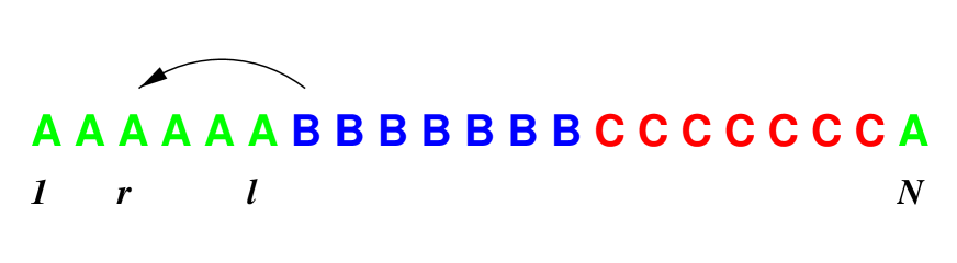
FIG. 2.: A ground state where $A_{1}=1,B_{r}=0$. In order to have $B_{r}=1$, it is necessary for a $B$ particle to travel a distance of $l-r+1$ into the $A$ domain.

(III) Ground states where $A_{1}=0,B_{r}=1$: again, since $r\leq N/3$ site $1$ has to be inside the $B$ domain. The values of $l$ satisfying this condition are in the range $2N/3+r\leq l\leq N$. In this case only excited states in which one of the $A$ walkers travels at least a distance $N-l+1$ into the $B$ domain will contribute to $\langle A_{1}B_{r}\rangle_{l}$. Hence we can use the upper bound $\langle A_{1}B_{r}\rangle_{l}\leq\sum_{s=N-l+1}^{\infty}{\cal Z}_{s}/{\cal Z}$, in this case. Therefore,

$$\sum_{l=2N/3+r}^{N}\langle A_{1}B_{r}\rangle_{l}\leq\sum_{l=2N/3+r}^{N}\sum_{s=N-l+1}^{\infty}q^{s}\;.$$ (38)

(IV) Ground states where $A_{1}=0,B_{r}=0$: there are three possibilities here. $(a)$ site $1$ is inside the $C$ domain and site $r$ is inside the $A$ domain ($N/3<l<N/3+r$), $(b)$ both the sites $1$ and $r$ are inside the $C$ domain ($r+N/3\leq l\leq 2N/3$), $(c)$ site $1$ inside the $B$ domain and site $r$ inside the $C$ domain ($2N/3<l<2N/3+r$). Since all these are consistent with $r\leq N/3$, all these cases can occur. It can be shown that the minimal energy needed to create an excited state where $A_{1}=1$ and $B_{r}=1$ is $\epsilon_{a}=2l-r-N/3-1$ for the case $(a)$, $\epsilon_{b}=N/3+r-3$ for the case $(b)$ and $\epsilon_{c}=5N/3-2l+r-1$ for the case $(c)$. The resulting expression for the bound is

$$\sum_{l=N/3+1}^{2N/3+r-1}\langle A_{1}B_{r}\rangle_{l}\leq\sum_{l=N/3+1}^{N/3+r-1}\sum_{s=\epsilon_{a}}^{\infty}q^{s}+\sum_{l=N/3+r}^{2N/3}\sum_{s=\epsilon_{b}}^{\infty}q^{s}+\sum_{l=2N/3+1}^{2N/3+r-1}\sum_{s=\epsilon_{c}}^{\infty}q^{s}\;.$$ (39)

The summations on the RHS of Eqs. (37-39) can be carried out explicitly. To leading order, the summations gives $q/(1-q)^{2}$ for each of Eqs. (37) and (38). The summation on the RHS of Eq. (39) vanishes exponentially in the thermodynamic limit. Using Eqs. (35-38), we get the following expression for the upper bound on $\langle A_{1}B_{r}\rangle$

$$\langle A_{1}B_{r}\rangle\leq\frac{1}{N}\left[r-1+\frac{2q}{(1-q)^{2}}+e^{-{\cal O}(N)}\right]\;.$$ (40)

Therefore $\langle A_{1}B_{r}\rangle={\cal O}(r/N)$. Similarly one can show that $\langle A_{1}C_{r}\rangle={\cal O}(1/N)$. Thus for all $q<1$, $\langle A_{1}A_{r}\rangle=1/3-{\cal O}(r/N)$, proving the existence of a complete phase separation.

IV Coarsening

A Monte Carlo Simulations

We have demonstrated that in the thermodynamic limit the system is phase separated when $N_{A}=N_{B}=N_{C}$. The general arguments given in section II indicate that when the global densities of the three species are non-vanishing and $q\neq 1$, the system phase separates, even when the three densities are not equal. The argument suggests that the typical time, $t_{f}$, in which the system leaves a specific phase separated configuration increases exponentially with the system size. Thus, a phase separated state is stable in the thermodynamic limit. In the following we use Monte Carlo simulations to support these arguments.

The time, $t_{f}$, can be measured using the auto-correlation function defined as,

$$c(t)=\frac{1}{N}\sum_{i=1}^{N}(\langle A_{i}(0)A_{i}(t)\rangle+\langle B_{i}(0)B_{i}(t)\rangle+\langle C_{i}(0)C_{i}(t)\rangle)\;,$$ (41)

where $A_{i}(t),B_{i}(t)$ and $C_{i}(t)$ are the values of the occupation variables $A_{i},B_{i}$ and $C_{i}$ at time $t$, and $\langle\ldots\rangle$ denotes an average over histories of evolution. Clearly, $c(0)=1$ while $c(\infty)=(N_{A}/N)^{2}+(N_{B}/N)^{2}+(N_{C}/N)^{2}$, the value of the autocorrelation between two independent configurations. Thus, $t_{f}$ may be defined as the decay time of $c(t)$ to $c(\infty)$ when at $t=0$ the system is totally phase separated.

We have measured the time scale $t_{f}$ using Monte Carlo simulations for different system sizes for $N_{A}=N_{B}=N_{C}$ and for $N_{A}\neq N_{B}\neq N_{C}$ for several $q$ values. An example of such measurements for $N_{A}/N=0.4$, $N_{B}/N=0.35$ and $N_{C}/N=0.25$ is presented in Fig. 3. In the plot $t_{f}$ is plotted versus system size for several values of $q$. It agrees with the exponential growth of $t_{f}$ with the system size suggested by the simple argument of section II. The same behavior seems to occur for all $q\neq 1$ and different choices of $N_{A}/N$, $N_{B}/N$ and $N_{C}/N$. Therefore we conclude that the Monte Carlo simulations support the claim that for any $q\neq 1$ the system will phase separate into three domains in the thermodynamic limit, even when the number of particles of each species is not equal. In the thermodynamic limit the translational symmetry is spontaneously broken in this state. Due to the slow dynamics, which reflects escape from metastable states, Monte Carlo simulations could be performed only for relatively small system size ($N\approx 100$). In order to study the coarsening process for larger systems we employ, in the following, a toy model which mimics the dynamics of the model (1). The toy model can be conveniently simulated for systems larger by about two orders of magnitude.

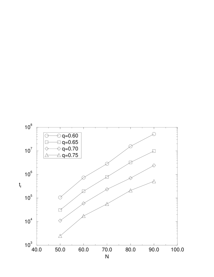
FIG. 3.: The decay time $t_{f}$ measured for different system sizes for several $q$ values. Here $N_{A}/N=0.4$, $N_{B}/N=0.35$ and $N_{C}/N=0.25$. The data is averaged over a 100 runs.

B Toy Model

We now construct a simple toy model which captures the essential physics of the coarsening process in the model at large times and enables us to simulate systems much larger than those accessible by Monte Carlo simulation. Using the toy model we examine another characteristic scale of the system. Namely, the average domain size $\langle l\rangle$ as a function of the time $t$. The results support the simple argument leading to a domain growth law $\langle l\rangle\sim\log t/|\log q|$. A mean-field version of the toy model is then solved analytically.

We consider a system at time $t$ such that the average domain size, $\langle l\rangle$, is much larger than the domain wall width. At these time scales, the domain walls can be taken as sharp and we may consider only events which modify the size of domains. This means that the dynamics of the system can be approximated by considering only the movement of particles between neighboring domains of the same species. Using this we represent a configuration by a sequence of domains of the form ${\rm\bf A}_{1}{\rm\bf B}_{1}{\rm\bf C}_{1}{\rm\bf A}_{2}{\rm\bf B}_{2}{\rm\bf C}_{2}\ldots{\rm\bf A}_{K}{\rm\bf B}_{K}{\rm\bf C}_{K}$, where the $i$th domain of, say $A$, particles is represented by ${\rm\bf A}_{i}$, as shown in Fig. 4. The exchange of particles between domains, say ${\rm{\bf A}}_{i}$ and ${\rm{\bf A}}_{i+1}$, takes place at a rate dictated by the size of the domains ${\rm{\bf B}}_{i}$ and ${\rm{\bf C}}_{i}$ which separate them. Since intermediate configurations of the form $\ldots{\rm\bf A}_{i-1}{\rm\bf B}_{i}{\rm\bf A}_{i}{\rm\bf C}_{i}\ldots$ rearrange on short time scales compared with the evolution between metastable states, only metastable configurations are considered in the toy model. Events in which a domain splits into two are ignored.

FIG. 4.: A configuration of the toy model represented by a sequence of domains.

Using these ideas we define the dynamics of the toy model as follows: at each time step two neighboring domains of the same species of particle are chosen randomly, say ${\rm\bf A}_{i}$ and ${\rm\bf A}_{i+1}$. Let $a_{i}$, $b_{i}$ and $c_{i}$ denote the lengths of the domains ${\rm\bf A}_{i},{\rm\bf B}_{i}$ and ${\rm\bf C}_{i}$ respectively. The length of the domain chosen is then modified by carrying out one of the following processes:

$$\begin{array}[]{ll}\left.\begin{array}[]{ll}1)&a_{i}\rightarrow a_{i}-1\\ &a_{i+1}\rightarrow a_{i+1}+1\\ \end{array}\right\}&{\rm with~{}rate}\quad q^{b_{i}}\\ &\\ \left.\begin{array}[]{ll}2)&a_{i}\rightarrow a_{i}+1\\ &a_{i+1}\rightarrow a_{i+1}-1\\ \end{array}\right\}&{\rm with~{}rate}\quad q^{c_{i}}\\ \end{array}$$ (42)

where, as before, $q<1$ is considered.

If $a_{i}$ becomes zero, then delete the domain ${\rm\bf A}_{i}$ from the list of domains, and merge ${\rm\bf B}_{i}$ and ${\rm\bf C}_{i}$ with ${\rm\bf B}_{i-1}$ and ${\rm\bf C}_{i-1}$, respectively. Then for $j>i$, shift the indices of the domains from $j$ to $j-1$, so that $K$ becomes $K-1$. The rules for updating ${\rm\bf B}$ and ${\rm\bf C}$ domains can be obtained from (42) using cyclic permutations and a slight change of indices.

Note that the toy model is only relevant to the description of the coarsening dynamics. This is because here, once the system is left with three domains, it remains in that state.

To simulate the toy model efficiently, an algorithm suitable for rare event dynamics must be used due to the small rate of events [25]. We use an algorithm which is performed by repeating the following steps:

1. List all possible events $\{n\}$ and assign to them rates $\{r_{n}\}$ according to the rules of the model.

2. Choose an event $m$ with probability $r_{m}/R$ where $R=\sum_{n}r_{n}$.

3. Advance time by $t\rightarrow t+\tau$, where $\tau=1/r_{m}$ .

The algorithm would be equivalent to a usual Monte Carlo simulation, where $1$ time step is equivalent to one Monte Carlo sweep, if in step $3$, $\tau$ would be drawn from a Poisson distribution $R~{}\exp[-R\tau]$. However, here we make an approximation by using the deterministic choice $\tau=1/r_{m}$.

We have simulated the dynamics for lattices of size up to $9000$. For simplicity we consider the case $N_{A}=N_{B}=N_{C}$. An example of a typical behavior of the average domain size as a function of $t$ is shown in Fig. 5. One can see that after an initial transient growth time the data fits very well with a $\log(t)$ behavior. Simulations for different $q$ values indicate that,

$$\langle l\rangle=a\log t/|\log q|$$ (43)

with $a\simeq 2.6$. The toy model enables one to verify the scaling behavior (43) and estimate the constant $a$. This would be very difficult to do by simulation of the full model (1).

FIG. 5.: Monte Carlo simulation results for the toy model for the average domain size, $\langle l\rangle$, vs. time ,$t$, for $N=9000$ and $q=0.8$. The data is averaged over 1760 runs.

C Mean Field Solution of the Toy Model

Here we present the solution of a mean-field version of the toy model based on ideas presented by Rutenberg and Bray [26] and Derrida et al.[27] in the study of the ordering dynamics in a one-dimensional scalar model. To construct the mean-field model we notice that since all steps in the toy model which involve exchange of particles between domains occur at a rate exponentially small in the size of domains, one can consider a model where dynamics occurs only in the vicinity of the smallest domains. The mean field approximation assumes that different domains are uncorrelated and does not distinguish between domains of different species. The second assumption relaxes the conservation of particles of each species. Thus, in contrast to the systems studied by [26] and [27] we do not expect the mean field to become exact in the scaling limit. We define the mean-field model as follows:

1. Pick one of the smallest domains $D_{\rm min}$.

2. Pick $2$ domains $D_{1}$ and $D_{2}$ randomly and treat them as the neighbors of $D_{\rm min}$.

3. Pick $3$ more domains randomly say, $D_{3},D_{4}$ and $D_{5}$.

4. Eliminate $D_{\rm min},D_{2}$ and $D_{3}$ from the system and change the length of the domains $D_{3},D_{4}$ and $D_{5}$ by

   $$l_{D_{3}} \rightarrow l_{D_{3}}+l_{D_{2}}$$ (44)

   $$l_{D_{4}} \rightarrow l_{D_{4}}+l_{D_{1}}$$ (45)

   $$l_{D_{5}} \rightarrow l_{D_{5}}+l_{D_{\rm min}}\;.$$ (46)

Steps $1$ to $4$ are performed simultaneously for all of the smallest domains in the system. Here $l_{D_{i}}$ is the length of domain $i$, and $l_{{\rm min}}$ is the length of the smallest domain. Steps $1$ to $3$ choose the smallest domain $D_{\rm min}$ and its nearest neighbors (see Fig. 6). Step $4$ uses the fact that the dynamics occur in the model only in the vicinity of the smallest domain and eliminates the three domains $D_{\rm min}$, $D_{1}$ and $D_{2}$ joining them appropriately with the other domains $D_{3}$, $D_{4}$ and $D_{5}$. Note that this mean-field dynamics does not take into account the time taken for these events to happen. This will be done later when we derive the growth law of domains.

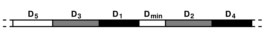
FIG. 6.: A configuration in the mean-field model after steps $1$ to $3$ have been performed for one of the smallest domains.

To solve the mean-field model we follow the method used in [26, 27]. Let $n_{l}(t)$ be the number of domains of size $l$, irrespective of the type of particle it consists of. Let $l_{\rm min}(t)$ be the length of the smallest domain and $M(t)=3K(t)$ be the total number of domains at time $t$. We will assume that $n_{l}(t)$ has the following scaling form in the large-time limit.

$$n_{l}=\frac{M}{l_{\rm min}}f(\frac{l}{l_{\rm min}})\;.$$ (47)

A solution of the model given in Appendix A yields $\langle l\rangle=\langle x\rangle l_{\rm min}$ where $\langle x\rangle$ is given by

$$\langle x\rangle=\frac{3e^{\gamma/3}}{\int_{0}^{\infty}dx~{}x^{-1/3}~{}e^{-x}~{}e^{-I(x)/3}}\;.$$ (48)

The growth law for $l_{\rm min}(t)$ can be derived following [26]: after the elimination of the smallest domain, $l_{\rm min}$ increases by $1$. This happens at a rate $q^{l_{\rm min}}/\langle l\rangle$, namely, the inverse time required by a typical domain to cross a distance $l_{\rm min}$ (thus, causing the annihilation of $D_{\rm min}$). Using $\langle l\rangle=\langle x\rangle l_{\rm min}$ we write

$$\frac{\partial l_{\rm min}}{\partial t}=\frac{q^{l_{\rm min}}}{\langle x\rangle l_{\rm min}}\;.$$ (49)

From this one can obtain the scaling form of the average domain size,

$$\frac{\langle l\rangle q^{-\langle l\rangle/\langle x\rangle}}{|\ln(q)|}\approx t\;.$$ (50)

Note that in this Eq. $\langle x\rangle$ does not depend, according to the mean-field solution, on either $t$ or $q$. One can see from (50) that for large $l$, $\langle l\rangle\approx\langle x\rangle\ln t/|\ln q|$ which was confirmed by the simulations of the toy model where $a=\langle x\rangle$ (see (43)). A numerical evaluation of (48) yields $\langle x\rangle\simeq 3.72$ as compared with $a=2.6$ obtained from the toy model simulations.

V Exact Results for Finite Systems

In section III the partition function, $Z_{N}$, and correlation function, $\langle A_{1}A_{r}\rangle$ for finite $r$, have been calculated in the thermodynamic limit. It is also of interest to obtain results for finite systems for the study of finite-size effects and the approach to the thermodynamic limit. Recently a matrix ansatz method has been introduced to study one-dimensional non-equilibrium systems [20]. It has been shown that in certain three-species models the steady-state weight and correlation functions can be represented as a product of matrices [11, 5, 12, 21]. In the ansatz a specific matrix is associated with each type of particle. Then the unnormalized probability of a certain configuration is obtained from a matrix product. The matrices corresponding to the different species of particles satisfy an algebra derived from the dynamics of the model. A scalar, i.e. the weight of a configuration or some correlation function, is usually obtained by performing a trace over the product of matrices, or by multiplying both sides of the product of matrices by vectors. Generalizing this method to replace matrices by tensors [28], we have been able to obtain recursion relations for the partition function and correlation function for finite systems for the special case $N_{A}=N_{B}=N_{C}$. The recursion relations are then used to obtain the partition function and correlation function $\langle A_{1}A_{r}\rangle$ for any $r$ in small systems. The results are used to study the scaling of the correlation function near the critical point $q=1$ (infinite temperature), where the typical domain wall width diverges.

A The Tensor Product Ansatz

It is convenient to consider the unnormalized weights, $f_{N}(\{X_{i}\})$, defined through

$$W_{N}(\{X_{i}\})=Z_{N}^{-1}f_{N}(\{X_{i}\})\;,$$ (51)

where $W_{N}(\{X_{i}\})$ is the probability of being in configuration $\{X_{i}\}$. The partition sum $Z_{N}$ is given by

$$Z_{N}=\sum_{\{X_{i}\}}f_{N}(\{X_{i}\})\;,$$ (52)

where the sum is over all configurations with $N_{A}=N_{B}=N_{C}$.

We generalize the matrix ansatz and construct the steady-state weight, $f_{N}(\{X_{i}\})$, from a product of tensors each corresponding to a particle located in a specific place on the lattice. The contraction of the tensors yields a tensor which is then contracted with ‘left’ and ‘right’ tensors to generate a scalar. The three tensors which represent the different type of particle are defined as rank $6$ tensors through the following tensor products of square matrices

$$\cal A = {\bf E}\otimes{\bf D}\otimes{\bf 1}$$ (53)

$$\cal B = {\bf 1}\otimes{\bf E}\otimes{\bf D}$$ (54)

$$\cal C = {\bf D}\otimes{\bf 1}\otimes{\bf E}\;.$$ (55)

Here ${\bf 1}$ is a unit matrix. The matrices ${\bf D}$ and ${\bf E}$ will be chosen in what follows to satisfy a commutation relation which will be dictated by the detailed balance condition.

To define $f_{N}(\{X_{i}\})$ we introduce the following notation: the contraction of two rank $6$ tensors $\mbox{\boldmath${\cal O}$ \unboldmath}={\bf O_{1}}\otimes{\bf O_{2}}\otimes{\bf O_{3}}$ and $\mbox{\boldmath${\cal P}$ \unboldmath}={\bf P_{1}}\otimes{\bf P_{2}}\otimes{\bf P_{3}}$, where ${\bf O_{i}}$ and ${\bf P_{i}}$ are square matrices, according to the rule ${\bf O_{1}P_{1}}\otimes{\bf O_{2}P_{2}}\otimes{\bf O_{3}P_{3}}$ is denoted by ${\cal OP}$ . The contraction of a rank 6 tensor ${\cal O}$ with a ‘left’ rank $3$ tensor $\langle{\cal K}|=\langle K_{1}|\otimes\langle K_{2}|\otimes\langle K_{3}|$, where $\langle K_{i}|$ are transposed vectors, and a ‘right’ rank $3$ tensor, $|{\cal M}\rangle=|M_{1}\rangle\otimes|M_{2}\rangle\otimes|M_{3}\rangle$, where $|M_{i}\rangle$ are vectors, defined through $\langle K_{1}|{\bf O_{1}}|M_{1}\rangle\langle K_{2}|{\bf O_{2}}|M_{2}\rangle\langle K_{3}|{\bf O_{3}}|M_{3}\rangle$ is denoted by $\langle{\cal K}|\mbox{ \boldmath${\cal O}$ \unboldmath}|{\cal M}\rangle$.

Using these definitions we write the steady-state weight of the system as

$$f_{N}(\{X_{i}\})=\langle{\cal U}|\prod_{i=1}^{N}[A_{i}\mbox{\boldmath$\cal A$ \unboldmath}+B_{i}\mbox{\boldmath$\cal B$ \unboldmath}+C_{i}\mbox{\boldmath$\cal C$ \unboldmath}]|{\cal V}\rangle\;,$$ (56)

where $A_{i}$, $B_{i}$ and $C_{i}$ are the occupation variables defined in (4). The expression states that a tensor $\cal A$ is present at place $i$ in the tensor product if site $i$ is occupied by an $A$ particle, a tensor $\cal B$ is present if site $i$ is occupied by a $B$ particle, and a tensor $\cal C$ is present if site $i$ is occupied by a $C$ particle. The action of the tensor product on $\langle{\cal U}|$ and $|{\cal V}\rangle$ (to be specified later) produces the scalar $f_{N}(\{X_{i}\})$.

It is straightforward to show using detailed balance that a necessary condition for Eq. (56) to be the steady-state weight is that the following commutation relations are satisfied between ${\cal A}$, ${\cal B}$, and ${\cal C}$ :

$$q\mbox{ \boldmath${\cal A}{\cal B}$\unboldmath} = {\cal B}{\cal A}$$ (57)

$$q\mbox{ \boldmath${\cal B}{\cal C}$\unboldmath} = {\cal C}{\cal B}$$ (58)

$$q\mbox{ \boldmath${\cal C}{\cal A}$\unboldmath} = \mbox{ \boldmath${\cal A}{\cal C}$ \unboldmath}\;.$$ (59)

Using (54) one can verify that these commutation relations are satisfied provided that $q{\bf DE}={\bf ED}$. This deformed commutator is of relevance in other stochastic systems [29, 30]. A representation of the matrices ${\bf D}$ and ${\bf E}$ which satisfies this commutation relation can be obtained as follows: let $\{\langle n|\}$ denote a basis set ($n=0,1,\ldots,N/3$) forming a vector space. In this basis we choose the matrices so that,

$$\langle n|{\bf E}=\langle n|q^{n}\;\;\;\;\;$$ for any

for ,

(60)

while for $n=0$, $\langle 0|{\bf D}=0$. An explicit form for ${\bf E}$ and ${\bf D}$ is given by the following $(N/3+1)\times(N/3+1)$ square matrices

$${\bf E}=\sum_{n=0}^{N/3}q^{n}|n\rangle\langle n|\;\;\;;\;\;\;{\bf D}=\sum_{n=1}^{N/3}|n\rangle\langle n-1|\;.$$ (61)

To obtain $f_{N}(\{X_{i}\})$, $\langle{\cal U}|$ and $|{\cal V}\rangle$ have to be specified. This should obviously be done so that $f_{N}(\{X_{i}\})$ is non-zero if the ansatz is to give a non-trivial result. We consider a general tensor product which corresponds to some configuration. The product has $N/3$ tensors of each type ${\cal A},{\cal B}$ and ${\cal C}$ , which results in a tensor product of three matrix products. Using (54) it can be seen that each matrix product contains $N/3$ matrices of each type ${\bf D}$, ${\bf E}$ and ${\bf 1}$. Since ${\bf E}$ and ${\bf 1}$ are diagonal, while ${\bf D}$ acts to its left as a lowering matrix (see (60)), choosing $\langle{\cal U}|=\langle N/3|\otimes\langle N/3|\otimes\langle N/3|\equiv\langle N/3,N/3,N/3|$, and $|{\cal V}\rangle=|0,0,0\rangle$ will give a non-zero $f_{N}(\{X_{i}\})$. This makes clear that the minimal size choice for the vector-spaces is $N/3+1$. Under this choice it is easy to see that in the ground states one has $f_{N}=q^{N^{2}/9}$ which corresponds to a ground state energy $N^{2}/9$. However, the choice of $\langle{\cal U}|$ and $\langle{\cal V}|$ is determined only up to some multiplicative factors. These factors may be used to shift the ground state energy of the system. For example choosing $\langle{\cal U}|$ as before with $|{\cal V}\rangle=q^{-N^{2}/9}|0,0,0\rangle$ will shift the ground state energy to $\mathrm{𝟎}$. In the following the factors are taken to be $1$.

Finally we would like to remark that usually when using the matrix ansatz for systems with periodic boundary conditions it is often convenient to use a trace of the matrix product [11, 21]. In this case this is not possible since the trace of our tensor product is always zero.

B Partition Sum

In terms of the ansatz (56) the partition function $Z_{N}$ is given by

$$Z_{N}=\langle\frac{N}{3},\frac{N}{3},\frac{N}{3}|(\mbox{\boldmath${\cal A}+{\cal B}+{\cal C}$\unboldmath})^{N}|0,0,0\rangle\;.$$ (62)

Note that we are using the canonical ensemble since all tensor products with unequal number of particles do not contribute to $Z_{N}$. This is easily seen since in these cases there are always more than $N/3$ ${\bf D}$ matrices acting on one of the vectors $\langle N/3|$.

To obtain the partition function we derive a recursion relation for

$$G_{i,j,k}^{l}\equiv\langle i,j,k|(\mbox{\boldmath${\cal A}+{\cal B}+{\cal C}$\unboldmath})^{l}|0,0,0\rangle\;.$$ (63)

One can see that $G_{N/3,N/3,N/3}^{N}=Z_{N}$. Rewriting $G_{i,j,k}^{l}$ as

$$G_{i,j,k}^{l} = \langle i,j,k|\mbox{ \boldmath${\cal A}({\cal A}+{\cal B}+{\cal C})$\unboldmath}^{l-1}|0,0,0\rangle+\langle i,j,k|\mbox{ \boldmath${\cal B}({\cal A}+{\cal B}+{\cal C}$ \unboldmath})^{l-1}|0,0,0\rangle$$ (65)

$$+\langle i,j,k|\mbox{ \boldmath${\cal C}({\cal A}+{\cal B}+{\cal C}$ \unboldmath})^{l-1}|0,0,0\rangle\;,$$

and using relations (54) and (60) the following recursion relation can be derived

$$G_{i,j,k}^{l}=q^{i}G_{i,j-1,k}^{l-1}+q^{j}G_{i,j,k-1}^{l-1}+q^{k}G_{i-1,j,k}^{l-1}\;.$$ (66)

The boundary conditions for this recursion relation is given by the no particle partition function $G_{i,j,k}^{0}=1$ if $i=j=k=0$ and is zero otherwise.

For small systems (up to $N=21$) for which the recursion relation is tractable analytically on Mathematica, we obtained the partition function $Z_{N}=G_{N/3,N/3,N/3}^{N}$ as a polynomial in $q$. As expected the first $N/3-2$ terms of the polynomial match the first $N/3-2$ terms of the expansion of (16) up to a factor of $q^{N^{2}/9}$ due to the energy shift in the ground state. For larger $N$ we solve the recursion relation numerically.

We note that (66) could have been derived directly from the definition of the partition function without recourse to the tensor ansatz. However, we believe the utility of the ansatz lies in the ease with which correlation functions can be manipulated and relations such as that of the next subsection derived.

C Correlation Functions

The correlation function $\langle A_{1}A_{r}\rangle$ is given in terms of the ansatz by

$$\langle A_{1}A_{r}\rangle=\frac{\langle\frac{N}{3},\frac{N}{3},\frac{N}{3}|\mbox{ \boldmath${\cal A}({\cal A}+{\cal B}+{\cal C})$ \unboldmath}^{r-2}\mbox{ \boldmath${\cal A}({\cal A}+{\cal B}+{\cal C})$ \unboldmath}^{N-r}|0,0,0\rangle}{Z_{N}}\;.$$ (67)

Using relations (54),(58) and (60) we obtain

$$\langle A_{1}A_{r}\rangle = q^{\frac{2N}{3}}\frac{\langle\frac{N}{3},\frac{N}{3}-2,\frac{N}{3}|(\mbox{\boldmath${\cal A}$ \unboldmath}+q\mbox{\boldmath${\cal B}$ \unboldmath}+\mbox{\boldmath${\cal C}$ \unboldmath}/q)^{r-2}(\mbox{\boldmath${\cal A}+{\cal B}+{\cal C}$ \unboldmath})^{N-r}|0,0,0\rangle}{Z_{N}}$$ (68)

$$= q^{\frac{2N}{3}}\frac{U(r)^{r}_{\frac{N}{3},\frac{N}{3}-2,\frac{N}{3}}}{Z_{N}}\;,$$ (69)

where we define the object $U(r)^{s}_{i,j,k}$ through,

$$U(r)^{s}_{i,j,k}=\langle i,j,k|(\mbox{\boldmath${\cal A}$ \unboldmath}+q\mbox{\boldmath${\cal B}$ \unboldmath}+\mbox{\boldmath${\cal C}$ \unboldmath}/q)^{s-2}(\mbox{\boldmath${\cal A}+{\cal B}+{\cal C}$ \unboldmath})^{N-s}|0,0,0\rangle\;.$$ (70)

A recursion relation for $U(r)^{s}_{i,j,k}$ can be obtained, similarly to the recursion relation for the partition function (66). Using (54) and (60) gives

$$U(r)^{s}_{i,j,k}=q^{i}U(r)^{s-1}_{i,j-1,k}+q^{j+1}U(r)^{s-1}_{i,j,k-1}+q^{k-1}U(r)^{s-1}_{i-1,j,k}\;.$$ (71)

The boundary conditions for the recursion relation are obtained by noting that $U(r)^{2}_{i,j,k}=\langle i,j,k|\mbox{ \boldmath$({\cal A}+{\cal B}+{\cal C})$\unboldmath}^{N-r}|0,0,0\rangle$, i.e., $U(r)^{2}_{i,j,k}=G_{i,j,k}^{N-r}$. Using the same methods one can obtain recursion relations for all other correlation functions.

The recursion relations are solved numerically for finite systems. This is done by first solving numerically for $G_{i,j,k}^{N-r}$, and then using the result as boundary conditions for the recursion relation (71). Owing to (69) we are ultimately interested in $U(r)^{r}_{N/3,N/3-2,N/3}$.

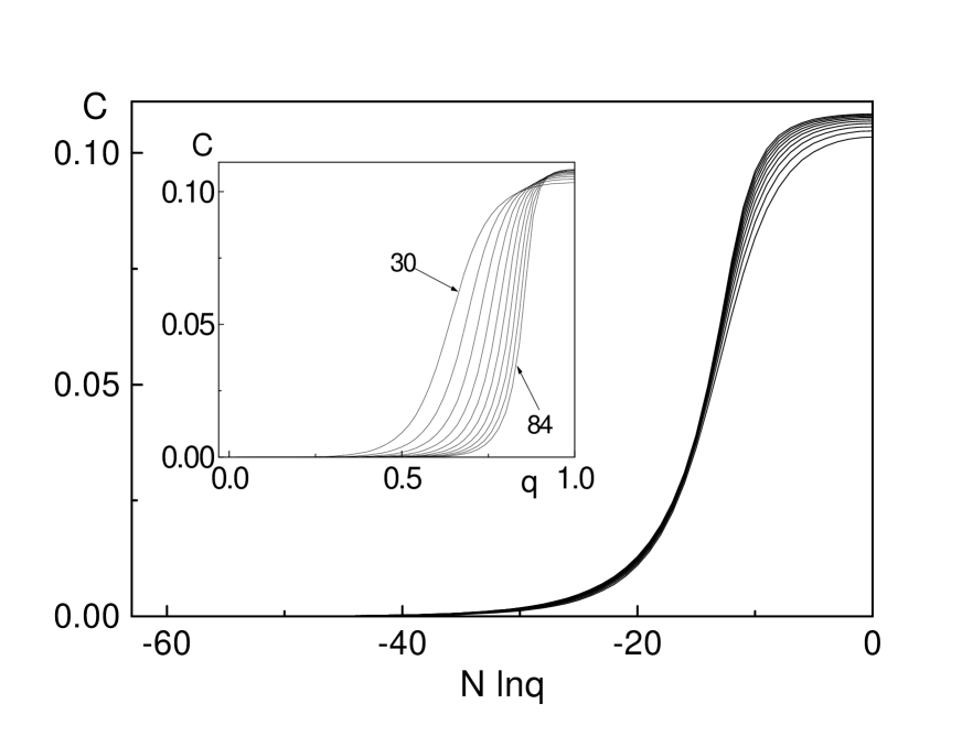
FIG. 7.: The correlation function $C=\langle A_{1}A_{N/2}\rangle$, obtained from the tensor ansatz, as a function of the scaled variable $N\ln q$ for $N=30,36,42,\ldots,84$. The inset shows the same data plotted against $q$.

Using these recursion relations we have calculated the correlation function $\langle A_{1}A_{N/2}\rangle$, which is a measure of the phase separation in the system, for various system sizes. When $\langle A_{1}A_{N/2}\rangle$ is close to zero the system is phase separated. In the disordered case, $q=1$, the value of the correlation function is $(N-3)/9(N-1)$, approaching $1/9$ in the thermodynamic limit. The results are shown in the inset of Fig. 7 one can see that the system is phase separated for small values of $q$ while for $q$ close to $1$ the system is disordered. The range of $q$ values for which the system is phase separated increases as the system size increases. The natural scaling variable near the critical point $q=1$ is $N\ln q$, the ratio between the domain size $N/3$ and the domain wall width $\int lq^{l}dl/\int q^{l}dl=1/|\ln q|$. In Fig.(7) the correlation function is plotted as a function of the scaling variable. One can see that the data collapse improves as the system size increases. This scaling variable was also suggested by the form of the partition function (16) in section III C.

VI Generalization to $M$ species

In the following we discuss possible generalization of the model to $M\geq 3$ species. To demonstrate how this might be done we first discuss the case $M=4$. We then comment briefly on $M>4$.

We now define a $4$-species model and argue that it phase separates. Consider a ring where each site is occupied by either an $A$, $B$, $C$ or $D$ particle. The model evolves according to the following procedure: at each time step two nearest neighbors are chosen randomly and exchanged according to the rates,

(72)

As before the model conserves the number of particles of each species. Note that several other generalizations of the model to four species are possible. However, for simplicity, we discuss only the model defined by (72) with $q<1$.

We now argue that the system phase separates into a configuration of the form $ABCD$ (where each letter now indicates a domain) as long as the densities of particles of each species are non-zero. Note that in the model $AB$, $BC$, $CD$, $DA$, $AC$ and $DB$ boundaries are stable while reverse boundaries $BA$, $CB$, $DC$, $AD$, $CA$ and $BD$ are unstable. As in the case of the three species model the system, starting from a random initial condition, evolves on a short time scale (i.e., which is not determined by the size of the system) into a metastable configuration where only stable domains are present. This configuration then slowly coarsens by slow diffusion of particles through neighboring domains. The system will finally reach the most stable state where the number of domains is minimal. One can easily check that this configuration is given by $ABCD$. Note that the system may exhibit other metastable states. For example, a state composed of $ACDABCD$ is also stable under the choice of rates (72). However, since this state is composed of more domains than the $4$-domain state, some of the domains are necessarily smaller. According to the argument presented in Section II the relaxation time of this sequence (proportional to $q^{-m}$ where $m$ is the typical domain size) is much shorter than the relaxation time of the $4$-domain state. Therefore the $4$-domain state is more stable so that the system will finally evolve into it.

In considering $M>4$ models one finds that for some choices of transition rates several states with the minimum number of domains may become metastable. For example, for $M=5$ it is possible to choose transition rates for which both $ABCDE$ and $ACEBD$ are locally stable. The relative stability (and thus the resulting phase separated state) may be found by determining the relaxation time of these states using simple considerations such as those presented in Section II.

As is the case of $M=3$ detailed balance is found to be satisfied for certain densities and transition rates for $M>3$. The condition for this is derived in Appendix B. In this case the relative stability of metastable states could be determined by comparing free energies.

VII Conclusion

In this paper a model of three species of particles diffusing on a ring previously introduced in [15] has been studied. The model is governed by local dynamics in which all moves compatible with the conservation of the three densities are allowed. We argue that phase separation should occur as long as all densities are non-zero. In the special case of equal densities we find that the steady state generated by the local stochastic dynamics is exactly given by a long-range asymmetric Hamiltonian. Phase separation for this case is explicitly demonstrated. The model provides an explicit example for the mechanism leading to phase separation or breaking of ergodicity in systems with local stochastic dynamics. Although we did not succeed in solving the steady state in the case of non-equal densities of particles, there is a strong evidence that phase separation still occurs. In order to investigate further the case of equal densities we employed a generalized matrix ansatz to calculate correlation function for finite-size systems. The novel structure of the ansatz may give some clue as to handle other $1d$ models which have so far resisted solution.

The dynamics of phase separation reduces to a coarsening problem where the typical domain size grows logarithmically in time. This results from the elimination of the domains at a rate exponentially small in their size. The slow dynamics poses a problem of how to access the scaling regime numerically. With direct numerical simulations only small systems can be studied (see Fig. 3). However, by employing a toy model in which domains rather than individual sites are updated one can simulate much larger systems and probe the scaling regime (see Fig. 5). Such ideas of updating domains have been used before in the study of coarsening [31]. With the aid of the toy model it should be possible to study other aspects of the scaling regime associated with the slow dynamics and escape from metastable states.

Generalizations are possible to models with $M>3$ species. We have discussed some possibilities and have shown that phase separation may take place, although the structure of the set of metastable states is more complicated. As was the case for $M=3$, conditions for detailed balance with respect to a long-range Hamiltonian may be determined.

The problem of phase separation and coarsening is of interest also in the broader context of phase transitions in one dimensional systems. Here the existence of conserved quantities results in certain local transition rates being zero. It would be interesting to generalize this study to models in which no conserved quantity exists and all local rates are non-vanishing. Also, another open problem is to calculate the steady state of the present model in the case of non-equal densities.

Acknowledgments: MRE is a Royal Society University Research Fellow and thanks the Weizmann Institute and the Einstein Center for warm hospitality during several visits. The support of the Minerva Foundation, Munich Germany, the Israeli Science Foundation, and the Israel Ministry of Science is gratefully acknowledged. Computations were performed on the SP2 at the Inter-University High Performance Computer Center, Tel Aviv. We thank S. Wiseman for helpful advice on programming and M. J. E. Richardson for careful reading of the manuscript.

A Mean-Field Solution of Toy Model

To solve the mean-field model we follow the method used in [26, 27]. Let $n_{l}(t)$ be the number of domains of size $l$, irrespective of the type of particle it consists of. Let $l_{\rm min}(t)$ be the length of the smallest domain and $M(t)=3K(t)$ be the total number of domains at time $t$. We will assume that $n_{l}(t)$ has the following scaling form in the large-time limit.

$$n_{l}=\frac{M}{l_{\rm min}}f(\frac{l}{l_{\rm min}})$$ (A1)

After the elimination of the smallest domain as given by (45), $n_{l},l_{\rm min}$ and $M$ change according to

$$M^{\prime} = M-3n_{l_{\rm min}}$$ (A2)

$$n^{\prime}_{l} = n_{l}(1-5\frac{n_{l_{\rm min}}}{M})+n_{l_{\rm min}}\frac{n_{l-l_{\rm min}}}{M}\theta(l-2l_{min})+2n_{l_{\rm min}}\sum_{j=l_{\rm min}}^{l-l_{\rm min}}\frac{n_{j}}{M}\frac{n_{l-j}}{M}$$ (A3)

$$l^{\prime}_{\rm min} = l_{\rm min}+1\;.$$ (A4)

Using the scaling form (A1) we have,

$$n^{\prime}_{l}=\frac{M^{\prime}}{l_{\rm min}+1}f(\frac{l}{l_{\rm min}+1})\approx\frac{M}{l_{\rm min}}[f(x)-(3f(1)+1)\frac{f(x)}{l_{\rm min}}-\frac{x}{l_{\rm min}}\partial_{x}f(x)]$$ (A5)

where $x=l/l_{\rm min}$ and we have expanded in $1/l_{\rm min}$. Now substituting these in (A3), it is straightforward to show that

$$f(x)+x\partial_{x}f(x)-2f(x)f(1)+f(1)f(x-1)\theta(x-2)+2\theta(x-2)f(1)\int_{1}^{\infty}dy~{}~{}f(y)f(x-y)=0\;.$$ (A6)

Using the Laplace transform,

$$\phi(p)=\int_{1}^{\infty}dx~{}~{}\exp[-px]~{}f(x)$$ (A7)

one can show that $\phi(p)$ satisfies the differential equation,

$$p\partial_{p}\phi(p)=f(1)[\phi(p)-1][2\phi(p)+e^{-p}]$$ (A8)

Since $\phi(p)=1-\langle x\rangle p+\ldots$, by expanding (A8) to order $p$ one obtains $f(1)=1/3$. The solution of (A8) with boundary conditions $\phi(0)=1$ and $\phi(p)\approx e^{-p}/3p$ for $p>>1$ is

$$\phi(p)=\frac{\int_{p}^{\infty}dx~{}~{}x^{-1/3}~{}e^{-x}~{}e^{-I(x)/3}}{3p^{2/3}e^{-I(p)/3}+\int_{p}^{\infty}dx~{}~{}x^{-1/3}~{}e^{-x}~{}e^{-I(x)/3}}$$ (A9)

where $I(x)=\int_{1}^{\infty}dt~{}~{}\exp[-xt]/t=-\log(x)-\gamma-\sum_{n=1}^{\infty}(-x)^{n}/(n!\ n)$ and $\gamma$ is the Euler constant. Inverse Laplace transform of (A9) gives the domain size distribution. From (A9) and using the expansion $\phi(p)=1-\langle x\rangle p+\ldots$, where the average is with respect to $f(x)$, we get

$$\langle x\rangle=\frac{3e^{\gamma/3}}{\int_{0}^{\infty}dx~{}x^{-1/3}~{}e^{-x}~{}e^{-I(x)/3}}\;.$$ (A10)

B Detailed Balance Condition for an M-Species Model

We now define the most general $M$ species model, where $M\geq 3$. Let $X_{i}$ denote a variable at site $i$ of a ring of size $N$, which takes values $X_{i}=1,2,\ldots,M$. $X_{i}=m$ means that site $i$ is occupied by a particle of type $m$. The system evolves by a random sequential, nearest-neighbor exchange dynamics, with the following rates:

$$mn~{}~{}{{q(m,n)\atop\longrightarrow}\atop{\longleftarrow\atop q(n,m)}}~{}~{}nm\;,$$ (B1)

and $q(X_{i},X_{i})=1$. The model conserves $N_{m}$, the number of particles of type $m$, for all $m$.

We now present a condition for the model to satisfy detailed balance with respect to the steady-state weight given by

$$W(\{X_{i}\})=\prod_{i=1}^{N-1}\prod_{j=i+1}^{N}q(X_{j},X_{i})\;,$$ (B2)

where the set $\{X_{i}\}$ describes the microscopic configuration.

Consider a particle exchange between sites $k$ and $k+1$, where $X_{k}=m,X_{k+1}=n$ and $k\neq N$ (i.e. in the bulk, note that site $1$ is chosen arbitrarily). Expanding the product in (B2), it is easy to verify that

$$\frac{W(X_{1},\ldots,m,n,\ldots,X_{N})}{W(X_{1},\ldots,n,m,\ldots,X_{N})}=\frac{q(n,m)}{q(m,n)}\;.$$ (B3)

Since this hold for any $m,n$, and is irrespective of the number of particles of each species, the steady-state weight (B2) satisfies detailed balance for all nearest-neighbor exchanges in the bulk. If the weights (B2) are translationally invariant then detailed balance will also hold for exchanges between sites $1$ and $N$.

Thus, to complete the proof of detailed balance it is sufficient to demand that (B2) is translationally invariant. To do this we relabel sites $i\rightarrow i+1$. The weight then becomes

$$W(\{X_{i}\})=\prod_{i=1}^{N-1}\prod_{j=i+1}^{N}q(X_{j-1},X_{i-1})\;,$$ (B4)

where $X_{0}$ is identical to $X_{N}$. Rewriting this equation by relabeling the indices we obtain,

$$W(\{X_{i}\})=\left[\ \prod_{i=1}^{N-1}\prod_{j=i+1}^{N}q(X_{j},X_{i})\ \right]\ \prod_{k=1}^{N-1}\frac{q(X_{k},X_{N})}{q(X_{N},X_{k})}\;.$$ (B5)

Comparing (B5) with (B2) and noting for example that,

$$\prod_{j=1}^{N}q(X_{j},X_{N})=\prod_{l=1}^{M}\left[q(l,X_{N})\right]^{N_{l}}\;,$$ (B6)

one can see that (B2) is translational invariant if

$$\prod_{l=1}^{M}\left[\frac{q(m,l)}{q(l,m)}\right]^{N_{l}}=1\;,$$ (B7)

for every $m=1,\ldots,M$. Thus, detailed balance holds if (B7) is satisfied. We note that for given densities $\{N_{m}\}$ the manifold of solutions for the rates is of $M(M-3)/2$ dimensions.

REFERENCES

- [1] see e.g. Scale Invariance, Interfaces and Non-equilibrium Dynamics. (eds. M. Droz, A. J. Mckane, J. Vannimenus and D. E. Wolf) Plenum, NY, (1995).
- [2] S. Katz, J. L. Lebowitz and H. Spohn, Phys. Rev. B 28, 1655 (1983); J. Stat. Phys. 34, 497 (1984).
- [3] B. Schmittmann and R. K. P. Zia Statistical Mechanics of Driven Diffusive Systems in Phase Transitions and Critical Phenomena (C. Domb and J. L. Lebowitz, eds.) Vol. 17 Academic Press, London, 1995.
- [4] L. D. Landau and E. M. Lifshitz Statistical Physics 1 (Pergammon, Oxford (1980)).
- [5] M. R. Evans, D. P. Foster, C. Godrèche and D. Mukamel Phys. Rev. Lett. 74, 208 (1995); J. Stat. Phys 80, 69 (1995).
- [6] C. Godrèche et al, J. Phys. A: Math. Gen. 28, 6039 (1995).
- [7] P. Gacs, J. Comput. Sys. Sci. 32, 15 (1986).
- [8] J. Kertész and D. E. Wolf Phys. Rev. Lett. 62 2571 (1989).
- [9] U. Alon, M. R. Evans, H. Hinrichsen and D. Mukamel Phys. Rev. Lett. 76 2746 (1996); cond-mat/9710142
- [10] S. A. Janowsky and J. L. Lebowitz, Phys. Rev. A 45, 618 (1992); G. Schütz, J. Stat. Phys. 73, 813 (1993).
- [11] B. Derrida, S. A. Janowsky, J. L. Lebowitz and E. R. Speer, Europhys. Lett. 22, 651 (1993); K. Mallick, J. Phys. A: Math. Gen. 29, 5375 (1996).
- [12] M. R. Evans, Europhys. Lett. 36, 13 (1996)
- [13] J. Krug and P. A. Ferrari, J. Phys. A: Math. Gen 29 L213 (1996)
- [14] R. Lahiri and S. Ramaswamy Phys. Rev. Lett. 79 1150 (1997).
- [15] M. R. Evans, Y. Kafri, H. M. Koduvely and D. Mukamel Phys. Rev. Lett. 80, 425, (1998).
- [16] B. Bergersen and Z. Rácz, Phys. Rev. Lett. 67, 3047 (1991).
- [17] F. J. Alexander and G. L. Eyink, cond-mat/9801258
- [18] P. F. Arndt, T. Heinzel and V. Rittenberg, J. Phys. A: Math. Gen. 31, L45, (1998).
- [19] F. Ritort Phys. Rev. Lett. 75, 1190 (1995); W. Krauth and M. Mézard Z. Phys. B 97, 127 (1995).
- [20] B. Derrida, M. R. Evans, V. Hakim and V. Pasquier J. Phys. A: Math. Gen. 26, 1493 (1993).
- [21] P. F. Arndt, T. Heinzel and V. Rittenberg, J. Phys. A: Math. Gen. 31, 833 (1998).
- [22] J. D. Shore, M. Holzer, and J. P. Sethna, Phys. Rev. B 46, 11376 (1992).
- [23] M. P. M. den Nijs in Phase Transitions and Critical Phenomena (C. Domb and J. L. Lebowitz, eds.) Vol. 12 Academic Press, London, 1988.
- [24] G. E. Andrews The Theory of Partitions, Encyclopedia of Mathematics and its Applications Vol. 2, p. 1–4 (Addison Wesley, MA, 1976).
- [25] A. B. Bortz, M. H. Kalos and J. L. Lebowitz, J. Comput. Phys. 17, 10 (1975).
- [26] A. D. Rutenberg and A. J. Bray Phys. Rev. E 50, 1900 (1994).
- [27] A. J. Bray, B. Derrida and C. Godrèche Europhys. Lett. 27, 175 (1994).
- [28] B. Derrida, M. R. Evans and K. Mallick, J. Stat. Phys. 79, 833 (1995).
- [29] M. J. E. Richardson J. Stat. Phys. 89, 777 (1997).
- [30] S. Sandow and G. Schütz Europhys. Lett. 26, 7 (1994).
- [31] S. J. Cornell and A. J. Bray, Phys. Rev. E 54, 1153 (1996).