Multiquantum Vortices in Conventional Superconductors with Columnar Defects Near the Upper Critical Field

Abstract

Equilibrium vortex configuration in conventional type II superconductors containing columnar defects is theoretically investigated. Near the upper critical field a single defect causes a strong local deformation of the vortex lattice. This deformation has $C_{3}$ or $C_{6}$ point symmetry, whose character strongly depends on the vortex-defect interaction. If the interaction is attractive, the vortices can collapse onto defect, while in the case of repulsion the regions free of vortices appear near a defect. Increasing the applied magnetic field results in an abrupt change of the configuration of vortices giving rise to reentering transitions between configurations with $C_{3}$ or $C_{6}$ symmetry. In the case of a small concentration of defects these transitions manifest themselves as jumps of magnetization and discontinuties of the magnetic susceptibility.

PACS: 74.60.Ge; 74.62.Dh

I Introduction

Mixed state or Shubnikov phase [1] of type II superconductors is characterized by penetration of vortices into the sample [2] each one carrying the superconducting flux quantum $\phi_{S}=\pi\hbar c/e$. A single vortex has a normal core with radius of order $\xi(T)$ (the coherence length at temperature $T$) surrounded by a closed superconducting current occupying the tube with radius $\lambda(T)$ (the penetration length). Near the upper critical field $H_{c2}$ these vortices form a triangular Abrikosov lattice [2]. If an external current is applied, vortices start to move due to the Lorentz force. This motion leads to an energy dissipation. Different kinds of defects, such as dislocations, point defects or regions with different superconducting properties create some additional field acting on the vortices. As a result vortices are pinned and nondissipative current of finite amplitude can flow through the superconducting sample. There are two different types of pinning [3]. Weak defects lead to the so-called collective pinning [4]. In this regime the vortex lattice is slightly deformed. This deformation is well described by elasticity theory [5, 6, 7, 4]. Strong defects lead to a single-particle pinning [4]. A single strong defect is able to pin a vortex and, at a finite defect concentration, formation of metastable states is possible [8]. A detailed theory of vortex pinning in conventional type II superconductors was formulated by Larkin and Ovchinnikov (see review paper [3]).

The discovery of high-temperature superconductivity [9] resulted in a deep understanding of the new rich and fundamental properties of vortex systems (see an exhaustive review papers of Blatter et. al. [10] and Brandt [11] and references therein). Statistical mechanics of vortices was formulated and new concepts appeared such as melting of the vortex lattice, vortex liquid and vortex glass. The usage of heavy ion irradiation for preparation of superconducting samples with columnar defects [12] opened new experimental possibilities to study the properties of vortex matter. Columnar defects serve as strong pinning centers, each of which is able to pin a single vortex as a whole. The radius of the columnar defect could be less than the Abrikosov lattice constant $a$ near $H_{c2}$. Such defects are referred to as short-range ones.

Strong columnar defects with radius $L$ much larger than the coherence length may lead to the formation of multiquantum vortices in high temperature superconductors [13]. Such vortices were observed experimentally on submicron artificial holes in mutlilayers $Pb/Ge$ [14]. Multiquantum vortices can also be formed at large pinning centers with radius of order of the penetration length [15]. In this paper we show that columnar defects can also strongly affect the properties of conventional type II superconductors. In such superconductors near the upper critical field even the short-range columnar defects cause a strong local deformation of the vortex lattice due to its softening and as a result to the formation of multiquantum vortices.

In the main part of the paper we consider a superconductor containing a single short-range columnar defect. When the magnetic field approaches to $H_{c2}$ the strength of the defect effectively increases resulting in strong lattice deformation in its vicinity. Initially the Abrikosov lattice is triangular. Therefore the local deformation belongs to one of the two possible symmetry types – $C_{6}$ or $C_{3}.$ In the case of an attractive defect, the vortices can collapse onto this defect with increasing of a magnetic field. As a result, reentering transitions between two local symmetries are possible. For example, at some external field the local vortex configuration $C_{6}$ with a single vortex pinned by a defect is preferred over the $C_{3}$ configuration with the defect placed at the center of a triangle. But with increasing of a magnetic field the closest three vortices in the $C_{3}$ configuration could collapse onto the defect and a $C_{6}$–$C_{3}$ transition occurs. Now the mostly preferred local configuration is of $C_{3}$ type, with a three-quantum vortex on the defect. Further increasing of a magnetic field results in a $C_{6}$ type configuration with a seven-quantum vortex at the defect and so on. In the case of a small concentration of defects (which was realized in an experiment [12], where the radius of the defect is equal to $2.5$ nm and the average distance between defects is $4,600$ nm). These transitions manifest themselves as jumps of magnetization and discontinuties of the magnetic susceptibility curve.

The present paper is organized as follows. In the second section we formulate the problem. Further, in the third section we study the relatively simple case of small deformation of the vortex lattice. It is realized for weak defects or for values of the magnetic field which are not very close to $H_{c2}$. The results of this study enable us 1) to scale the defect parameters with the magnetic field, and 2) to predict the occurrence of symmetry change when the applied magnetic field increases. The central section IV containes the results of the numerical solution of the pertinent equations. Here we present a universal phase diagram of the superconductor near the upper critical field, and analyze the vortex lattice deformation as a function of the magnetic field for various defect parameters. The next section V is devoted to the case of small concentration of the defects. Here we estimate the high order concentration corrections with respect to defect and study the magnetization and the magnetic susceptibility behavior near the upper critical field. Section VI summaries the main results. In the Appendix, the Abrikosov lattice expansion in terms of the first Landau level wave functions is obtained for an arbitrary position of the lattice with respect to the origin.

II Formulation of the Problem

Consider a superconductor containing columnar defects and subject to an external magnetic field ${\bf H}=H\hat{z}.$ Both the defect column axis and the magnetic field are assumed to be directed along the $z$-axis. The unit volume thermodynamic potential of such a superconductor at a fixed temperature $T$ close to the critical temperature $T_{c}$ can be written as

$$F=\frac{1}{S}\int f\left({\bf r};\left[\alpha,\gamma,\Psi,{\bf A}\right]\right)d{\bf r},$$ (1)

where ${\bf r}$ is the two dimensional (2D) position vector and the Ginzburg–Landau density $f$ of the thermodynamic potential [16] is

$$f\left({\bf r};\left[\alpha,\gamma,\Psi,{\bf A}\right]\right)=\alpha({\bf r})|\Psi({\bf r})|^{2}+\frac{\beta}{2}|\Psi({\bf r})|^{4}+\gamma({\bf r})\left|{\bf\partial}_{-}\Psi({\bf r})\right|^{2}+\frac{1}{8\pi}({\bf B({\bf r})}-{\bf H})^{2}.$$ (2)

Here $\Psi({\bf r})$ and ${\bf A}({\bf r})$ are the order parameter and 2D vector potential respectively,

$${\bf B}=\hat{z}\left(\frac{\partial A_{y}}{\partial x}-\frac{\partial A_{x}}{\partial y}\right),$$

and $\partial_{-}$ is the gauge invariant gradient

$${\bf\partial}_{-}\equiv-i\hbar\frac{\partial}{\partial{\bf r}}+\frac{2e}{c}{\bf A}.$$ (3)

The space dependent Ginzburg–Landau coefficients $\alpha({\bf r})$ and $\gamma({\bf r})$ for defects placed at the points $\{{\bf r}_{j}\}$ have the form

$$\alpha({\bf r})=\alpha_{0}+\sum_{j}\alpha_{1}({\bf r}-{\bf r}_{j}),$$

$$\gamma({\bf r})=\gamma_{0}+\sum_{j}\gamma_{1}({\bf r}-{\bf r}_{j}),$$

where $\alpha_{0}<0$ and $\gamma_{0}>0$ correspond to a uniform superconductor and the short-range functions $\alpha_{1}({\bf r})$ and $\gamma_{1}({\bf r})$ describe the perturbation of these coefficients caused by a columnar defect located at the origin.

According to the standard procedure one has to minimize the density (2) (i.e. to solve the Ginzburg–Landau equations), to find the extremal order parameter $\Psi$ and vector potential ${\bf A}$ and to substitute them into the formula (1). Assume now that the density $n$ of defects is small, $n\xi^{2}(T)\ll 1$, i.e. the average distance between defects $n^{-1/2}$ is much larger than the coherence length $\xi(T)$ (which is of order of the distance $a$ between neighboring vortices of the Abrikosov lattice). In this case the concentration expansion [17] of the thermodynamic potential density in linear approximation yields

$$F=f^{A}+n\int(f_{1}({\bf r})-f^{A})d{\bf r}.$$ (4)

Here

$$f^{A}=-\frac{1}{8\pi}\frac{(H-H_{c2})^{2}}{(2\kappa^{2}-1)\beta_{A}},$$ (5)

is the free energy of the Abrikosov triangular lattice, $\beta_{A}=1.1596$ [18] and $f_{1}({\bf r})$ is the minimum of the density (2) containing a single defect placed at the origin $(\alpha({\bf r})=\alpha_{0}+\alpha_{1}({\bf r}),\phantom{aa}\gamma({\bf r})=\gamma_{0}+\gamma_{1}({\bf r}))$. Near the upper critical field

$$H_{c2}=\frac{|\alpha_{0}|c}{2\gamma_{0}\hbar e},$$

corresponding to a uniform superconductor with $\alpha({\bf r})=\alpha_{0},$ $\gamma({\bf r})=\gamma_{0},$ the minimization procedure can be applied to the density of the thermodynamic potential

$$f_{1}\left({\bf r};\left[\alpha,\gamma,\Psi\right]\right)=\alpha_{0}\left(1-h\right)|\Psi|^{2}+\frac{\beta}{2}\left(1-\frac{1}{2\kappa^{2}}\right)|\Psi|^{4}+\alpha_{1}({\bf r})|\Psi|^{2}+\gamma_{1}({\bf r})|{\bf\partial}_{-}^{0}\Psi|^{2},$$ (6)

which depends only on the order parameter [19, 4]. Here $h\equiv H/H_{c2},$ $\kappa$ is the Ginzburg–Landau parameter

$$\kappa=\frac{c}{4\hbar e\gamma_{0}}\sqrt{\frac{\beta}{2\pi}},$$

and $\partial^{0}_{-}$ is defined by Eq.(3) where the vector potential ${\bf A}_{0}$ of an applied field ${\bf H}$ stands for ${\bf A}$. In what follows we will use the vector potential in the symmetric gauge ${\bf A}_{0}=H(-y/2,x/2)$.

To find the order parameter which realizes this minimum one can use an expansion of $\Psi$ in terms of Landau functions $L_{k}(x,y)$ (A4) of the lowest Landau level of a particle with electron mass and the charge $-2e$ in the magnetic field $H,$ substitute this expansion into Eq.(6) and find the expansion coefficients from the minimum condition [8]. Such an expansion serves as a good approximation and one can neglect the contribution of the highest Landau levels even at a field $H=0.5H_{c2}$ [20]. In linear concentration approximation the problem is reduced to a single defect problem. Therefore in the case of isotropic functions $\alpha_{1}(r)$ and $\gamma_{1}(r)$ the symmetry of the unperturbed Abrikosov lattice enables us to consider only two cases corresponding either to $C_{6}$ symmetry, or to $C_{3}$ symmetry. The hexagonal symmetry corresponds to the distorted vortex lattice with one vortex placed on the defect. The trigonal one corresponds to the lattice with the defect located in the center of the vortex triangle. In the hexagonal case the trial order parameter can be written as

$$\Psi_{6}(x,y)=i\sum_{k=0}^{\infty}\left[\pi^{-1}M_{6}(k)+D(k)\right]L_{k}(x,y).$$ (7)

Here $D(k)$ are the variational parameters which should be found. The case when all $D$ are equal to zero and only the coefficients $M_{6}(k)$ remain, corresponds to the order parameter $\Psi_{6}^{A}(x,y)$ which describes the Abrikosov lattice with one of the vortices located at the origin and one of the symmetry axes parallel to the $x$-axis. The coefficients $M_{6}(k)$ (see Eq.(A6) of Appendix) are real and obey the selection rule [8] $k=6K+1,\phantom{aa}K=0,1,2,...\phantom{aa}.$ In the trigonal case the trial order parameter is written as

$$\Psi_{3}(x,y)=\sum_{k=0}^{\infty}i^{-k}\left[\pi^{-1}M_{3}(k)+D(k)\right]L_{k}(x,y).$$ (8)

The case when all $D$ are equal to zero, corresponds to the order parameter $\Psi_{3}^{A}(x,y)$ which describes the Abrikosov lattice whose origin coincides with the center of the vortex triangle and one of the symmetry axes is parallel to the $x$-axis. The real coefficients $M_{3}(k)$ (A8) obey the selection rule $k=3K,K=0,1,2,...\phantom{aa}.$

Thus to obtain the lattice deformation caused by a single defect we have to find separately the extremal set of the variational parameters $D(k)$ within each of the two symmetry classes separately, and to choose the most preferable one from the two of them. This procedure and its consequences will be discussed in the next two sections.

III Weak Defects

Consider first a system with weak defects (in a sense that will be clear later on). It is natural to assume that in this case the two last terms in the thermodynamic potential density (6) do not contribute to the variational equation for the order parameter and the latter one coincides with its Abrikosov value $\Psi^{A}.$ Accordingly, the equilibrium thermodynamic potential can be written as

$$F=f^{A}+n\int(\alpha_{1}({\bf r})|\Psi^{A}|^{2}+\gamma_{1}({\bf r})|{\bf\partial}_{-}^{0}\Psi^{A}|^{2})d{\bf r}.$$ (9)

Let us then specify the functions $\alpha_{1}({\bf r})$ and $\gamma_{1}({\bf r})$ which describe the perturbation of the Ginzburg-Landau coefficients by defects

$$\alpha_{1}({\bf r})=-\alpha_{0}\tilde{\alpha}\exp\left(-\frac{r^{2}}{2L^{2}},\right)$$

$$\gamma_{1}({\bf r})=\gamma_{0}\tilde{\gamma}\exp\left(-\frac{r^{2}}{2L^{2}}\right).$$

Here $\tilde{\alpha}$ and $\tilde{\gamma}$ describe the strengths of the defect, measured in units $\alpha_{0}$ and $\gamma_{0}$ respectively, and $L$ is its size. Accurate estimations show that if the properly scaled strengths of defects

$$\alpha=\frac{\tilde{\alpha}}{1-h}$$ (10)

$$\gamma=\frac{\tilde{\gamma}h}{1-h}$$ (11)

are small, $\alpha,\gamma\ll 1,$ then one can indeed neglect the Abrikosov lattice distortion.

It seems that in the attractive case the preferable configuration is always a $C_{6},$ i.e. Abrikosov lattice with one of the vortices located on a defect. Nevertheless we will show that even in the case of small deformation, the previous statement is not always valid. In the general case one should take into account the two possible types of lattice symmetry with respect to a given defect, i.e. the two Abrikosov order parameters $\Psi_{6,3}^{A}$ corresponding to the $C_{6}$ symmetry

$$\Psi_{6}^{A}(x,y)=i\pi^{-1}\sum_{k=0}^{\infty}M_{6}(k)L_{k}(x,y),$$

and to the $C_{3}$ symmetry

$$\Psi_{3}^{A}(x,y)=\pi^{-1}\sum_{k=0}^{\infty}i^{-k}M_{3}(k)L_{k}(x,y).$$

Substitution of these order parameters in the Eq.(9) yields the corresponding thermodynamic potentials,

$$F_{6}=f^{A}+\frac{4\pi c}{3^{1/4}}\left|f^{A}\right|M_{6}^{2}(1)\gamma\varphi,$$ (12)

$$F_{3}=f^{A}+\frac{4\pi c}{3^{1/4}}\left|f^{A}\right|M_{3}^{2}(0)\alpha\varphi.$$ (13)

Here $\varphi$ is the dimensionless scaled defect size

$$\varphi=h\frac{L^{2}}{\xi^{2}(T)},$$ (14)

$c=na^{2}\sqrt{3}/2$ is the dimensionless defect concentration (the number of defects per a single vortex) and $a$ is the Abrikosov lattice constant (see Eq.(A2) below).

Suppose we deal with a defect in which the only variation parameter is $\tilde{\alpha}$ (i.e. the transition temperature). Then if $\tilde{\alpha}>0$ such defect increases the thermodynamic potential $F_{3}$ leaving the $F_{6}$ unchanged (13). This means that the defect attracts a vortex and the symmetry $C_{6}$ is preferable. Obviously, in the opposite case $\tilde{\alpha}<0$ the symmetry $C_{3}$ is preferable and therefore the defect is repulsive. This confirms the qualitative speculations presented in the Introduction. But the question is what happens if variation of both $\tilde{\alpha}$ and $\tilde{\gamma}$ is allowed. To answer this question we must compare the correction terms in Eqs.(13). Taking values of $M_{6}(1)$ and $M_{3}(0)$ from the Tables I, II of Appendix we conclude that if

$$\gamma\leq 0.387\alpha,$$ (15)

then the symmetry $C_{6}$ is preferable (attractive case). Yet, the ratio $\alpha/\gamma$ grows with the magnetic field (see Eq.(11) above). Therefore if, for some field, $\gamma$ is slightly less than $0.387\alpha$ then further increasing of a magnetic field can violate the inequality (15) and causes a first order phase transition to the $C_{3}$ symmetry.

In the region of field considered above, the vortex lattice is comparatively rigid and vortex repulsion dominates above vortex-defect interaction. However even in this region the type of the lattice symmetry can be changed. For stronger magnetic fields or for stronger defects the lattice deformation near defect is not negligible any more. This leads to richer and more complicated properties of the vortex system even in the case when $\tilde{\gamma}=0$.

IV Strong Deformation of the Vortex Lattice

Now consider the case when a lattice deformation near defects is essential. This deformation is completely described by an infinite set of variational parameters $\{D(k)\}$. Direct substitution of the test function $\Psi(x,y)$ expressed in the forms (7) or (8) into the expression for the thermodynamic potential (4), (6) yields

$$F=f^{A}\left[1-\frac{4\pi c}{3^{1/4}}Q\right],$$ (16)

where

$$Q=\frac{2}{3^{1/4}\beta_{A}}\left\{\sum_{k,l,m}\frac{(l+m)!}{2^{l+m+2}\sqrt{k!l!m!(l+m-k)!}}\left[\pi D^{*}(k)D(l)D(m)D^{*}(l+m-k)+\right.\right.$$ (17)

$$\left.2M(l+m-k)(D(k)D^{*}(l)D(m)+c.c.)\right]+2\sum_{k,l}I(k,l)D^{*}(k)D(l)+$$ (18)

$$\left.\frac{1}{2}\sum_{k,l}\sqrt{\frac{(k+l)!}{k!l!}}J(k+l)(D(k)D(l)+c.c)\right\}+\sum_{k}|D(k)|^{2}+$$ (19)

$$\sum_{k}|\pi^{-1}M(k)+D(k)|^{2}\frac{\varphi^{k}}{(1+\varphi)^{k}}\left[\alpha\varphi+\gamma(\varphi^{2}+k(1+2\varphi^{2}))\right],$$ (20)

and

$$I(k,l)=\sum_{m}\frac{(l+m)!}{\sqrt{k!l!m!(l+m-k)!}}\frac{M(m)M(l+m-k)}{2^{l+m+1}\pi},$$

$$J(k)=\sum_{m}\sqrt{\frac{k!}{m!(k-m)!}}\frac{M(m)M(k-m)}{2^{k+1}\pi}.$$

This expression for the correction to the thermodynamic potential is general and valid for both two symmetries $C_{6}$ and $C_{3}$. In each of these cases one should take into account the selection rules

$$M_{3}(k)=\delta_{k,3K}M_{3}(3K),$$ (21)

$$M_{6}(k)=\delta_{k,6K+1}M_{6}(6K+1),$$ (22)

$$K=0,1,2,...\phantom{a},$$ (23)

and use for $M_{3,6}(k)$ their corresponding (real) values (see Eqs.(A6), (A8) below). The next step is the minimization of the thermodynamic potential (16), (20) with respect to the coefficients $\{D(k)\}$. The equations which determine $\{D(k)\}$ have the form

$$\frac{2}{3^{1/4}\beta_{A}}\left\{\sum_{l,m}\frac{(l+m)!}{2^{l+m+1}\sqrt{k!l!m!(l+m-k)!}}(\pi D(l)D(m)D^{*}(l+m-k)+M(l+m-k)D(l)D(m))\right.$$ (24)

$$\left.\sum_{l,m}\frac{(k+m)!M(k-l+m)}{2^{k+m}\sqrt{k!l!m!(k-l+m)!}}D(l)D^{*}(m)+\sum_{l}\left[2I(k,l)D(l)+\sqrt{\frac{(k+l)!}{k!l!}}J(k+l)D^{*}(l)\right]\right\}$$ (25)

$$-D(k)+\left(\pi^{-1}M(k)+D(k)\right)\frac{\varphi^{k}}{(1+\varphi)^{k}}\left[\alpha\varphi+\gamma(\varphi^{2}+k(1+2\varphi^{2}))\right]=0$$ (26)

and were obtained by Ovchinnikov [8] who used their linearized version for studying possible structural transitions.

We numerically solve the infinite nonlinear system of Ovchinnikov equations without any simplification. The only (quite natural and verified) assumption which we use is that the perturbed lattice conserves its initial symmetry. This means that the coefficients $\{D(k)\}$ obey the same selection rules

$$D_{6}(k)=\delta_{k,6K+1}D_{6}(6K+1),$$

$$D_{3}(k)=\delta_{k,3K}D_{3}(3K),$$

$$K=0,1,2,...\phantom{a}.$$

that the initial coefficients $M(k)$ do. Our strategy is as follows. For fixed values of the parameters $\tilde{\alpha}$ and $\tilde{\gamma}$ and for a fixed magnetic field we calculate the coefficients $D(k)$ for two possible symmetries $C_{6}$ and $C_{3}.$ Then we substitute these solutions together with the corresponding sets of $\{M\}$ into Eq.(20) and choose the most preferable solution which determine the vortex lattice deformation as well as the thermodynamics of the system to first order in the low concentration approximation. Thus to understand the results obtained we should first analyze the behavior of the coefficients $D(k)$ in a magnetic field and to explain how this behavior influences to the order parameter evolution within each of the two symmetries separately. Then we can describe the vortex configuration, corresponding to the preferable solution for a fixed set of parameters $\tilde{\alpha},\phantom{a}\tilde{\gamma},\phantom{a}L,$ and its evolution in a magnetic field.

The qualitative information concerning the behavior of the coefficients $D(k)$ in a magnetic field can be obtained directly from Eqs.(26). Consider for example an attractive defect with $\tilde{\alpha}>0$ and $\tilde{\gamma}=0.$ In this case, if one is not too close to the critical field $H_{c2}$ the hexagonal symmetry should be realized and one starts from an analysis of the $C_{6}$ solutions. Due to selection rules, the first nonvanishing equation of the system (26) will correspond to the value $k=1$. This equation strongly depends on the (scaled) defect parameters $\alpha,$ $\gamma$ and $\varphi$, which are collected in the last term of Eq.(26). But right in the next equation (which corresponds to the value $k=7$) this term is proportional to $\varphi^{7}$ and due to the short range nature of the defect $(\varphi\leq 1$) is very small. Therefore all the higher order equations (26) with $k=13,19,...$ are practically homogeneous. As a result, the solution of (26) will give nonzero coefficients $D(k)$ only for some small values of $k$. Thus the deformation of a vortex lattice happens mainly near the defect, at the distance of order of the Larmor radius $R_{k}\propto\sqrt{k_{max}}$  corresponding to the largest value of $k$ such that $D(k_{max})\neq 0$, while the rest of the lattice remains undistorted.

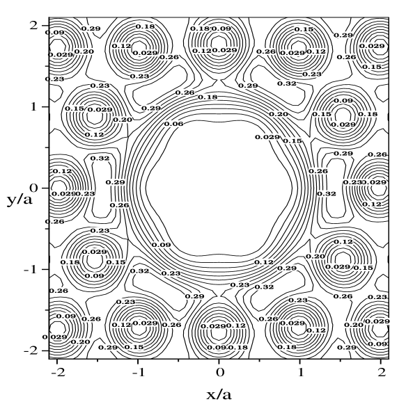
FIG. 1.: The dimensionless square modulus of the order parameter $\Delta$ in the hexagonal case for parameters $\tilde{\alpha}=0.5,\tilde{\gamma}=0.0,\varphi/h=0.5,h=0.93$. Seven vortices collapse on the defect.

With raising of the applied magnetic field the effective coupling constants $\alpha$ and $\gamma$ increase drastically (see Eq.(11)), while the parameter $\varphi$ (14) does not undergo any visible change. This leads to increasing values of the higher coefficients $D(k)$ in the expansion (7) of the order parameter and as a result, to spreading of the deformation far from the defect.The further the growth of the magnetic field is, the larger are the effective coupling constants. This implies that the last term in the Eq.(26) for $k=1$ becomes much larger than all preceding terms. In this case the solution is $D_{6}(1)=-\pi^{-1}M_{6}(1),$ i.e. the first expansion coefficient practically reaches its limiting value. This value completely compensates the contribution of the unperturbed Abrikosov lattice to the $k=1$ expansion coefficient in Eq.(7). In this region of fields the expansion (7) begins from $k=7$. The order parameter in the nearest vicinity of the defect becomes

$$\Psi\propto r^{7}e^{7i\vartheta}.$$

This means that the six nearest vortices have (almost) collapsed on the defect which pins the vortex containing seven flux quanta. One can see this effect on fig.1. Here the quantity

$$|\Delta_{6}|^{2}=\frac{\sqrt{3}|\Psi_{6}|^{2}}{2\pi|C|^{2}},$$ (27)

which is proportional to the square modulus of the order parameter (normalization constant $C$ is defined by Eq.(A3)), is plotted.

With the further increasing the applied field the next coefficients $D_{6}(7),$ $D_{6}(13)$, and so on will reach their limiting compensation values $-\pi^{-1}M_{6}(7),$ $-\pi^{-1}M_{6}(13),$ … , and one could principally get a vortex containing thirteen, nineteen an so on flux quanta. However, numerical calculations show that for a realistic field range (not extremely close to the upper critical field) only the first collapse can be realized.

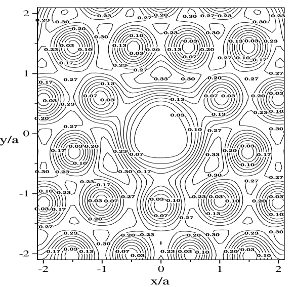
FIG. 2.: The dimensionless square modulus of the order parameter $\Delta$ in the trigonal case for parameters $\tilde{\alpha}=0.5,\tilde{\gamma}=0.0,\varphi/h=0.5,h=0.85$. Three vortices collapse on the defect.

A similar behavior of the expansion coefficients $\{D(k)\}$ takes place in the trigonal case $C_{3}.$ Here in the case of attraction the coefficient $D_{3}(0)$ is the first one which reaches its compensation value $-\pi^{-1}M_{3}(0),$ that corresponds to the three vortices collapse on the defect. Such a configuration is displayed on fig.2 where the quantity $|\Delta_{3}|^{2}$ defined by the r.h.s of Eq.(27), with $\Psi_{6}$ replaced by $\Psi_{3}$, is plotted for the same values of parameters as in the hexagonal case and for the applied field $h\approx 0.85$. With increasing of the magnetic field one expects the appearance of six-, and so on multy-quanta vortices. As in the previous case, numerical analysis shows that only the first collapse happens in a realistic range of field.

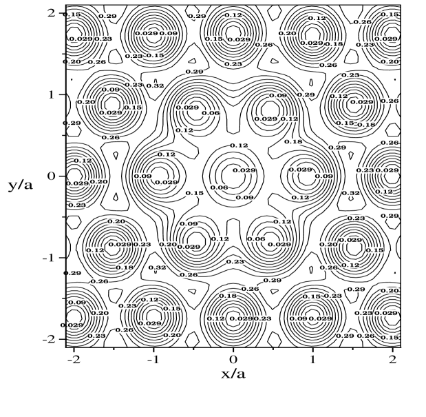
FIG. 3.: The dimensionless square modulus of the order parameter $\Delta$ in the hexagonal case for parameters $\tilde{\alpha}=0.5,\tilde{\gamma}=0.0,\varphi/h=0.5,h=0.85$. Attractive defect causes a comparatively weak vortex lattice deformation.

Note that for the same set of parameters the first collapse within the trigonal symmetry occurs at a weaker field ($h\approx 0.85$) than in the hexagonal symmetry ($h\approx 0.93$). The reason is that in the $C_{6}$ system seven vortices must overcome their mutual repulsion in order to fall on the defect, while in the $C_{3}$ system only three vortices collapse. For the field $h\approx 0.85$, at which, in the symmetry $C_{3},$ three vortices are already collapsed on the defect (fig.2), in the $C_{6}$ symmetry, the lattice is distorted but still without any vortex collapse (fig.3).

The vortex lattice deformation near a repulsive defect is presented in fig.4. Here the three nearest vortices are slightly shifted from the defect and a visible deformation occurs only in the nearest vicinity of the defect.

Up to now we analyzed the solutions of Eqs.(26) within two symmetries $C_{6}$ and $C_{3}$ separately. Now we can choose the most preferable one from them and describe the typical vortex lattice behavior in some interval of the magnetic fields close to the upper critical field. We start from the same case of attractive defects $\tilde{\alpha}>0$ ($\tilde{\gamma}$=0) of a small concentration. If an applied field is not too close to $H_{c2}$, then a deformation of the lattice near a single deffect is small and the preferable local symmetry near each defect is $C_{6}.$ The defects are occupied by vortices and the rest of the lattice is slightly deformed. With increasing of the magnetic field the deformation near defects becomes stronger (as shown in fig.3) and at some critical field $h_{1}$ the $C_{3}$ solution of Eqs.(26) corresponding to collapse of three vortices on the defect becomes preferable (see fig.2). As a result, a local structural transition $C_{6}$ $\rightarrow$ $C_{3}$ occurs. With further increasing of the field, one deals with $C_{3}$ symmetry, three vortices occupying the defect and the deformation of the nearest (with respect to the defect) part of the vortex lattice is observed. But at some critical field $h_{2}$ the $C_{6}$ solution of Eqs.(26) corresponding to collapse of seven vortices on the defect (see fig.1) becomes preferable and a local structural transition $C_{3}$ $\rightarrow$ $C_{6}$ occurs and so on. Thus, one has a sequence of reentering first order phase transitions $C_{6}\rightarrow C_{3}\rightarrow C_{6}\rightarrow...$ .

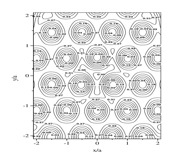
FIG. 4.: The dimensionless square modulus of the order parameter $\Delta$ in the hexagonal repulsive case for parameters $\tilde{\alpha}=-0.5,\tilde{\gamma}=0.0,\varphi=0.5$.

A similar analysis can be done in the general case where $\tilde{\alpha}\neq 0$ and $\tilde{\gamma}\neq 0$. The numerical results obtained for various sets of parameters and magnetic field enables us to construct a phase diagram in the $(\alpha,\gamma)$ plane for a fixed scaled size $\varphi$ (14) of a defect. Part of such diagram is given in fig.5. Here the two solid curves separate the regions where the local symmetry is hexagonal $(C_{6})$ or trigonal $(C_{3})$ . Near the upper critical field $\varphi\approx L^{2}/\xi^{2}$ and the diagram becomes universal. For each fixed defect parameters and for each value of the magnetic field the diagram enable us to determine the preferable local symmetry of the system.

To explain how to extract this information from the phase diagram consider a sample with some fixed parameters $\tilde{\alpha}$, $\tilde{\gamma}$, and $L$, and start from an initial applied field $h_{0}\equiv H_{0}/H_{c2}$. This corresponds to a starting point $(\alpha_{0},\gamma_{0})$ in the diagram of fig.5, where $\alpha_{0}$ and $\gamma_{0}$ are determined by Eqs.(11) with $h=h_{0}$. Further evolution of the parameters $\alpha$ and $\gamma$ with growth of the magnetic field is described by equation

$$\gamma=\frac{\tilde{\gamma}}{\tilde{\alpha}}\left(\alpha-\alpha_{0}\right)+\gamma_{0}$$

and corresponds to some ray on the phase diagram, starting at the initial point $(\alpha_{0},\gamma_{0})$ and directed out of the origin. Four such rays are displayed in fig.5. For all rays the starting field is $h_{0}=0.9$ and $\tilde{\alpha}=0.1$. The increasing of the magnetic field leads to the change in the effective coupling constants (11) i.e. to the motion of a starting point along the ray. This movement in its turn results in a sequence of reentering transitions from one local symmetry to another.

FIG. 5.: Phase diagram of superconductor on ($\alpha,\gamma$) plane. All rays: $\tilde{\alpha}=0.1;h_{0}=0.9.$ Solid ray $\tilde{\gamma}=0.01$. Dashed ray $\tilde{\gamma}=0.03$. Dotted ray $\tilde{\gamma}=0.06$. Dashed-dotted ray $\tilde{\gamma}=-0.01.$

The solid ray corresponds to $\tilde{\gamma}=0.01$. It is seen from fig.5 that at the initial field $h_{0}=0.9$ the local deformation has a $C_{6}$ symmetry. This is consistent with the analytical prediction of Section III: the deformation around a defect is small and the inequality (15) is valid. As the field increases, the ray crosses the lower solid curve and the sample undergoes a first order phase transition to the trigonal local symmetry $C_{3}$. At this symmetry we have three collapsed vortices at each defect. Transition to the symmetry $C_{6}$ back is also possible, but it is not seen on the diagram because it occurs in the region $\alpha\gg 1$ i.e. at a field extremely close to the upper critical field $H_{c2}$.

The dashed ray corresponds to the value $\tilde{\gamma}=0.03$ and represents probably the most interesting case. Here even in the comparatively low field $h\approx 0.775<h_{0}$ (the corresponding point of the ray is not displayed on fig.5) the $C_{6}$-$C_{3}$ symmetry transition occurs. In both the two lattice configurations below and above the transition the lattice deformation is small and can be described within the approach of Section III. The inequality (15) is violated below the transition field and is valid above it. The dashed ray on the diagram starts from the field $h_{0}=0.9$ and for the first time crosses the lower solid curve at a field $h\approx 0.906$, at which the lattice undergoes the next $C_{3}$ $\rightarrow$ $C_{6}$ transition. No vortex collapse still happens at this field because the value of $D_{6}(1)$ is still far from its compensating value. However two next transitions take place because of vortex collapse. The second transition to the symmetry $C_{3}$ at a field $h\approx 0.94$ happens when the coefficient $D_{3}(0)$ in the symmetry $C_{3}$ almost reaches its compensating value $D_{3}(0)=-\pi^{-1}M_{3}(0)$ and therefore this transition corresponds to the collapse of the three vortices at the defect. Similarly the third transition to the symmetry $C_{6}$ at a field $h\approx 0.99$ corresponds to the collapse of the seven vortices at the defect.

The dotted ray in fig.5 corresponds to $\tilde{\gamma}=0.06$ that provides only a $C_{3}$ symmetry in the comparatively low field region. In the high field region we obtain $C_{3}$ $\rightarrow$ $C_{6}$ transition at the field $h\approx 0.98$.

Note that the figures 2 and 3 already reffered to above, present the contour plots of the order parameter near defect in the vicinity of the $C_{6}$ $\rightarrow$ $C_{3}$ transition due to collapse of the three nearest vortices on the defect. These plots correspond to the point $(\approx 4,0)$ on the ray coinciding with the positive $\alpha-$semiaxis on the phase diagram. At this point the order parameter exhibits a small deformation in the symmetry $C_{6}$ as it is displayed in fig.3, while in the symmetry $C_{3}$ it is strongly deformed due to the collapse (see fig. 2).

In the region where $\alpha>0$ and $\gamma<0$ a local symmetry transition $C_{6}\rightarrow C_{3}$ due to vortex collapse is described by the last fourth ray on the diagram. This ray corresponds to the parameters $\tilde{\alpha}=0.1$, $\tilde{\gamma}=-0.01$.

V Small concentration of the defects

During the two previous sections we dealt with a single defect problem. To be sure that our results (16) do describe a macroscopic system with a finite concentration of the defects we have to be sure that the next (second order) concentration correction to the thermodynamic potential is small. To estimate this correction one has to solve exactly the two defects problem which is much more complicated. Therefore we choose another way.

Consider for simplicity an attractive case and magnetic field which is not too close to $H_{c2}.$ Put the undistorted vortex lattice on the plane where (point) defects are distributed and shift one of the vortices nearest to each inhomogeneity to the position of that inhomogeneity. There are many similar ways to arrange the vortex lattice, but one has to choose such a way which leads to alternation of the regions where the lattice is compressed with ones where its rarefied. Finally let us distort the regions of the lattice close to inhomogeneities according to the results obtained within single defect approximation. This latter distortion is already taken into account exactly. So one has only to estimate the additional contribution to the thermodynamic potential from the intermediate regions (between inhomogeneities) whose deformation is well described by elastic theory.

The number of extra vortices per region is of order of unity. Therefore the deformation tensorup to a numerical factor of the order of unity equals to dimensionless concentration of defects $c$. The correction to the thermodynamic potential will be of the order of $Cc^{2}$, where $C$ is the elastic modulus. But the elastic part of the deformation has an alternating behavior with a characteristic wavelength of the order of the average distance between inhomogeneities. As it was shown by E. Brandt [7], all the elastic moduli are proportional to $(1-H/H_{c2})^{2}$ if this distance is much less than the penetration length divided by $(1-H/H_{c2})^{1/2}$. The latter inequality can be rewritten as $36\kappa c\gg 1-H/H_{c2}$, where $\kappa\gg 1$ is the Ginzburg-Landau parameter. In the region of parameters which we are mostly interested in $c=0.03$, $1-H/H_{c2}=0.06$ and the inequality $\kappa\gg 1$ is evidently valid. This means that corresponding contribution to the thermodynamic potential is of the order of $(1-H/H_{c2})^{2}c^{2}$. This is exactly the second order concentration correction which in the case $c\ll 1$ is smaller than the contribution accounted for within the linear concentration expansion.

Thus in the case of small concentration one can use the results obtained in the two previous sections and describe the thermodynamics of the system near $H_{c2}$. Define a dimensionless magnetization

$$m\equiv-4\pi(2\kappa^{2}-1)\beta_{A}\frac{M}{H_{c2}}$$

and dimensionless magnetic succeptibility

$$\chi=\frac{\partial m}{\partial h}.$$

FIG. 6.: The magnetization curve of superconductor for the parameters $\tilde{alpha}=0.1,\tilde{\gamma}=0.03$ and for the concentration values $c=0.03$ (triangles) and $c=0.05$ (circles).

All the local symmetry transitions described above manifest themselves as jumps on the magnetization curve (fig.6) and as discontinuities on the magnetic succeptibility curve (fig.7). The most pronounced jumps occur at the two transitions accompanied by vortex collapse, namely at the fields $h\approx 0.94$ and $h\approx 0.99$.

FIG. 7.: The magnetic succeptibility of superconductor for the parameters $\tilde{alpha}=0.1,\tilde{\gamma}=0.03$ and for the concentration values $c=0.03$ (triangles) and $c=0.05$ (circles).

VI Summary

We studied the equilibrium properties of conventional type II superconductor with small concentration of randomly placed identical columnar defects. In the vicinity of the upper critical field the vortex lattice undergoes a strong deformation with two possible local symmetries – hexagonal one $C_{6}$ and trigonal one $C_{3}$. The character of the deformation is determined by the vortex-defect interaction. The vortices can collapse onto attractive defects and the formation of multy-quanta vortices becomes possible. Formation of the multiquantum vortices was predicted earlier [15], but in ”twice” opposite limiting case. We deal with a short-range defect and gain an energy because of softening of the Abrikosov lattice near $H_{c2},$ while in [15] a very strong defect with a radius comparable with the penetration length was considered.

Increasing the external field gives rise to the reentering transitions between the two possible types of symmetry. These transitions can be described by a universal phase diagram. They manifest themselves as jumps of the magnetization and peculiarities of the magnetic susceptibility.

One of the way to observe these equilibrium states near $H_{c2}$ is to cool a sample subject to a magnetic field in the normal state, below the critical temperature. Another possibility is to observe not the equilibrium state as a whole, but visualize the local deformation of the vortex lattice near defects.

VII Acknowledgements

This study was partially supported by the Israel Science Foundation. We are grateful to H. Brandt, E. Chudnovsky, B. Horovitz, V. Mineev, R. Mints, Z. Ovadyahu, B.Ya. Shapiro, and E. Zeldov for very helpful discussions of our results.

A Abrikosov Lattice Expansion

The Abrikosov order parameter [2]

$$\Psi^{A}(x,y)=C\exp\left[-\frac{2\pi}{\sqrt{3}}\frac{y^{2}}{a^{2}}\right]\theta_{3}\left(\left.\frac{x}{a}-i\frac{y}{a}-\frac{1}{4}\right|e^{i\frac{\pi}{3}}\right),$$

which was obtained in the Landau gauge ${\bf A}=\hat{x}H(-y,0)$ describes a triangular vortex lattice with sites

$$\left\{\begin{array}[]{c}x=a(2m+n+2)/2,\\ y=a\sqrt{3}(2n+1)/4,\end{array}\right.$$

($m$ and $n$ are integers). Here

$$a(T)=2\xi(T)\sqrt{\frac{\pi}{h(T)\sqrt{3}}}$$ (A2)

is the triangle side (Abrikosov lattice constant), and $h(T)\equiv H/H_{c2}(T).$ The Abrikosov normalization constant $C$ is related to the thermodynamic potential density (5) of the clean superconductor by

$$|C|^{2}=\frac{3^{1/4}2|f^{A}|}{|\alpha_{0}|(1-h)},$$ (A3)

and $\theta_{3}(u|\tau)$ is the Euler $\theta$ -function [21].

The order parameter

$$\Psi_{x_{0},y_{0}}(x,y)\equiv\exp\left[-i\frac{2\pi}{\sqrt{3}a^{2}}xy+i\frac{4\pi y_{0}}{\sqrt{3}a}x\right]\Psi^{A}(x-ax_{0},y-ay_{0}),$$

describes the shifted Abrikosov lattice in the symmetric gauge. This order parameter can be expanded as

$$\Psi_{x_{0},y_{0}}(x,y)=\pi^{-1}\sum_{k=0}^{\infty}M_{x_{0},y_{0}}(k)L_{k}(x,y)$$

with respect to Landau functions with the orbital moment $k\geq 0$

$$L_{k}(x,y)=\frac{C}{3^{1/4}}\sqrt{\frac{2\pi}{k!}}\left[\frac{\sqrt{2\pi}}{3^{1/4}}\frac{r}{a}\right]^{k}\exp\left[-ik\vartheta-\frac{\pi r^{2}}{\sqrt{3}a^{2}}\right],$$ (A4)

of the lowest Landau level of a particle with electron mass and charge $-2e$ in the magnetic field $H.$ The expansion coefficients are

$$M_{x_{0},y_{0}}(k)=\sqrt{\frac{\sqrt{3}\pi}{2}}\sum_{n=-\infty}^{\infty}\sum_{m=0}^{k-2m\geq 0}\frac{i^{k-2m}\left[\sqrt{2\pi\sqrt{3}}\right]^{k-2m}}{2^{m}m!(k-2m)!}\left(n+\frac{2y_{0}}{\sqrt{3}}\right)^{k-2m}\times$$

$$\exp\left\{i\frac{\pi}{2}\left[n^{2}-n(1+4x_{0})\right]-\frac{\pi\sqrt{3}}{2}\left(n+\frac{2y_{0}}{\sqrt{3}}\right)^{2}\right\}.$$

The case $x_{0}=-1/2$, $y_{0}=-\sqrt{3}/4$ corresponds to the $C_{6}$ symmetry when one vortex is placed at the origin. Taking into account the selection rule (23) we write down the expansion coefficients as

$$M_{-1/2,-\sqrt{3}/4}(k)=i\delta_{k,6K+1}M_{6}(6K+1),$$

where

$$M_{6}(k)=\sqrt{\frac{\sqrt{3}\pi}{2}}\sum_{n=-\infty}^{\infty}\sum_{m=0}^{k-2m\geq 0}\frac{i^{k-2m-1}\left[\sqrt{2\pi\sqrt{3}}\right]^{k-2m}}{2^{m}m!(k-2m)!}\left(n-\frac{1}{2}\right)^{k-2m}\times$$ (A5)

$$\exp\left\{i\frac{\pi}{2}\left[n^{2}+n\right]-\frac{\pi\sqrt{3}}{2}\left(n-\frac{1}{2}\right)^{2}\right\}.$$ (A6)

The expansion coefficients $M_{6}(k)$ are real. The values of the first few of them are contained in the table I.

TABLE I.: Values of an Expansion Coefficients $M_{6}(k)$

$k$	$M_{6}(k)$
$1$	$-2.792$
$7$	$4.057$
$13$	$2.260$
$19$	$-4.852$
$25$	$-1.494$
$31$	$-3.538$
$37$	$4.817$
$43$	$2.605$
$49$	$0.479$
$55$	$5.180$

The second case $x_{0}=-1/2$ and $y_{0}=\sqrt{3}/12$ corresponds to the $C_{3}$ symmetry, when the origin of the coordinate system is placed in the center of an elementary triangle. Selection rules allow us to write down the expansion coefficients as

$$M_{-1/2,\sqrt{3}/12}(k)=i^{-3K}\delta_{k,3K}M_{3}(3K).$$

The explicit expression for $M_{3}(k)$ is given by the formula

$$M_{3}(k)=\sqrt{\frac{\sqrt{3}\pi}{2}}\sum_{n=-\infty}^{\infty}\sum_{m=0}^{k-2m\geq 0}\frac{i^{2k-2m}\left[\sqrt{2\pi\sqrt{3}}\right]^{k-2m}}{2^{m}m!(k-2m)!}\left(n+\frac{1}{6}\right)^{k-2m}\times$$ (A7)

$$\exp\left\{i\frac{\pi}{2}\left[n^{2}+n\right]-\frac{\pi\sqrt{3}}{2}\left(n+\frac{1}{6}\right)^{2}\right\}.$$ (A8)

All the coefficients $M_{3}(k)$ also are real. The values of the first few coefficients are given by Table II.

TABLE II.: Values of an Expansion Coefficients $M_{3}(k)$

$k$	$M_{3}(k)$
$0$	$1.738$
$3$	$-2.942$
$6$	$-2.227$
$9$	$1.646$
$12$	$-3.568$
$15$	$-2.310$
$18$	$-0.756$
$21$	$3.185$
$24$	$-1.563$
$27$	$3.110$
$30$	$3.606$

REFERENCES

- [1] L.V. Shubnikov, V.I. Khotkevich, Yu.D. Shepelev, Yu.N. Ryabinin, Zh. Eksper. Teor. Fiz. 7, 221 (1937).
- [2] A.A. Abrikosov, Sov. Phys. JETP 5, 1174 (1957).
- [3] A.I. Larkin, Yu.N. Ovchinnikov, in Nonequilibrium Superconductivity, Eds. D.N. Landerberg and A.I. Larkin (Elsevier, Amsterdam, 1986).
- [4] A.I. Larkin and Yu.N. Ovchinnikov, J. Low Temp. Phys. 34, 409 (1978).
- [5] R. Labusch, Phys. Stat. Sol. 32, 439 (1969).
- [6] A.I. Larkin, Sov. Phys. JETP 31, 784 (1970).
- [7] E. H. Brandt, J. Low Temp. Phys. 26, 709, 735 (1977).
- [8] Yu.N. Ovchinnikov, Sov. Phys. JETP 55, 1162 (1982).
- [9] J.G. Bednortz, K.A. Muller, Z. Phys. 64, 189 (1986).
- [10] G. Blatter,M.V. Feigelman, V.B. Geshkenbein, A.I. Larkin, V.M. Vinokur, Rev. Mod. Phys. 66,1125 (1994).
- [11] E.H. Brandt, Rep. Progr. Phys. 58, 1465 (1995)
- [12] a) L. Civale, A.D.Marwick, M.W. McElfresh, T.K. Worthington, A.P. Malozemoff, F.H. Holtzberg, J.R. Thompson, M.A. Kirk, Phys. Rev. Lett. 65, 1164 (1990); b) L. Civale, A.D.Marwick, T.K. Worthington, M.A. Kirk, J.R. Thompson, L. Krusin-Elbaum, Y. Sun, J.R. Clem, F.H. Holtzberg, Phys. Rev. Lett. 67, 648 (1991).
- [13] A.I. Buzdin, Phys. Rev. B 47 11416 (1993)
- [14] M. Baert, V.V. Metlushko, R. Jonckheere, V.V. Moshchalkov, Y. Bruynseraede, Phys. Rev. Lett. 74, 3269 (1995).
- [15] I.B. Khalfin, B.Ya. Shapiro, Physica C 202, 393 (1992).
- [16] V.L. Ginzburg, L.D. Landau, Zh. Eksper. Teor. Fiz. 20, 1064 (1950).
- [17] I.M. Lifshits, Nuovo Cimento 3, Suppl., 716 (1963).
- [18] W.M. Kleiner, L.M. Roth, S.H. Autler, Phys. Rev. A133, 1226 (1964).
- [19] E.H. Brandt, Phys. Stat. Sol. (b) 71, 277 (1975).
- [20] E.H. Brandt, Phys. Stat. Sol. (b) 51, 345 (1972).
- [21] I.S. Gradstein, and I.M. Ryzhik, Tables of Integtrals, Sums, Series and Products (Academic, New York, 1980).