Inelastic quantum transport in superlattices: success and failure of the Boltzmann equation

Abstract

Electrical transport in semiconductor superlattices is studied within a fully self-consistent quantum transport model based on nonequilibrium Green functions, including phonon and impurity scattering. We compute both the drift velocity-field relation and the momentum distribution function covering the whole field range from linear response to negative differential conductivity. The quantum results are compared with the respective results obtained from a Monte Carlo solution of the Boltzmann equation. Our analysis thus sets the limits of validity for the semiclassical theory in a nonlinear transport situation in the presence of inelastic scattering.

Quantum mechanical description of electrical transport in strong electric fields is a notoriously difficult subject. As the distribution function of the electrons deviates strongly from equilibrium, the standard approaches of linear response do not apply. In some circumstances heated distribution functions may be useful, but in principle such an assumption should be justified by an underlying theory. Usually this problem of hot electrons is treated within the semiclassical Boltzmann transport equation (BTE) which can be solved to a desired degree of numerical accuracy by Monte-Carlo simulations (MC) [1]. This way both the distribution function and the current density can be obtained for arbitrary field strengths. Nevertheless one has to be aware of the severe assumptions implied by the use of the BTE. The electrons are viewed as classical particles with a dispersion relation given by the band structure and scattering is treated using Fermi’s golden rule where energy conservation is strict. To recover the BTE from a quantum transport theory, such as nonequilibrium Green functions (NGF)[2], several assumptions are required (see e.g. [3, 4]): (i) spectral functions with finite width are replaced by $\delta$-functions for free particles, (ii) the nonequilibrium Green function is assumed to be expressible in terms of the momentum distribution function, (iii) retardation effects are neglected to reproduce the Markovian collision integral [5]. Attempts to relax some of these assumptions have been made in earlier studies [6, 7], and quantum corrections to distribution functions have been reported. Nevertheless we are not aware of any direct comparison of the results from BTE with a full quantum transport theory far from equilibrium, which is the task of this paper.

Semiconductor superlattices (SL)[8] provide a unique opportunity to study effects related to quantum transport because the width of the miniband can be tailored by the choice of the barrier and well widths as well as the material composition. For sufficiently large electric fields negative differential conductivity (NDC) appears which can be understood within the semiclassical theory by electrons traversing the whole miniband[9] thus performing Bloch-oscillations both in momentum and real space. This gives a distribution function which is far from any kind of thermal equilibrium. Many papers have analyzed the solution of the BTE in this miniband transport regime[10]. Alternatively, in the NDC region the electrical transport can be formulated in terms of Wannier-Stark hopping[11]. Finally, for small miniband width $\Delta$ and strong scattering, the transport can be viewed as a sequential tunneling process between adjacent wells[12].

While these simplified approaches have proven to be useful to analyze different experimental situations, it is clear that a complete description of transport in SLs requires a more sophisticated quantum mechanical treatment such as density matrix theory [13, 14] or NGF [15]. Recently it was shown that a calculation based on NGF reproduces the results of the simplified approaches and determines their respective ranges of validity[16]. All these approaches employed a specific (heated) thermal distribution to model the in-scattering processes. While this can be a reasonable approximation for the evaluation of averaged quantities such as the current density, such an assumption is certainly not justified if the nonequilibrium electron distribution function itself is of interest.

In this work we calculate the drift velocity-field relation as well as the electron distribution function both in a quantum transport model based on NGF and within the BTE under stationary conditions. Identical system parameters and scattering matrix elements for impurity and phonon scattering are used. Our NGF calculation provides us with a full self-consistent solution of the transport problem within the self-consistent Born-approximation for the scattering. (Thus, effects of higher order scattering such as weak localization are neglected.) This approach is similar to recent calculations for the resonant tunneling diode [17]. The BTE is solved by a MC-simulation. Its results can be easily interpreted in terms of standard concepts such as electron heating and Bloch-oscillating electrons. We find excellent agreement between the drift velocities calculated semiclassically and quantum mechanically in the range of validity for the miniband transport discussed in Refs. [16, 18]. On the other hand, the failure of the BTE becomes obvious if the potential drop per period $eFd$ or the scattering width $\hbar/\tau_{\rm scatt}$ become larger than the miniband width $\Delta$.

We consider a semiconductor superlattice with period $d$ and restrict ourselves to nearest neighbor coupling. The band structure reads $E(q,{\bf k})=2T_{1}\cos(qd)+E_{k}$ with $T_{1}=-\Delta/4$ and $E_{k}=\hbar^{2}k^{2}/2m$. Here $q$ denotes the Bloch vector in the growth direction, which is restricted to $-\pi/d<q\leq\pi/d$, and ${\bf k}$ is the two-dimensional Bloch vector perpendicular to the growth direction. $m=0.067m_{e}$ is the effective mass of the conduction band of GaAs. We restrict ourselves to the lowest miniband neglecting all phenomena related to intersubband processes (e.g., the second peak in the drift velocity-field relation at higher fields [8, 12]).

Three types of scattering processes are included: Impurity scattering at $\delta$-potentials with density $N_{d}$ (per unit area) and constant matrix element $V_{\rm imp}$ leading to a scattering rate $1/\tau_{\rm imp}=N_{d}\pi V_{\rm imp}^{2}\rho_{0}/\hbar$, where $\rho_{0}$ is the two-dimensional density of states. (The impact of further elastic scattering processes like interface roughness can be taken into account by applying a reduced value of $\tau_{\rm imp}$.) Optical phonons of energy $\hbar\omega_{\rm o}=36$ meV with a constant matrix element $M_{\rm o}$. We choose $M_{\rm o}$ such that the rate for spontaneous emission of a phonon (if allowed) is given by $1/\tau_{\rm o}=\pi M_{\rm o}^{2}\rho_{0}/\hbar=8$ ps^-1. These values are realistic for GaAs. In order to achieve energy relaxation for energies lower than $\hbar\omega_{\rm o}$ we mimic acoustic phonons by a second phonon with constant energy $\hbar\omega_{\rm a}$. The ratio $\omega_{\rm o}/\omega_{\rm a}$ should be irrational to avoid spurious resonances and we choose $\hbar\omega_{\rm a}=\hbar\omega_{\rm o}(\sqrt{5}-1)/10\approx 4.4498$ meV. The constant matrix element $M_{\rm a}$ was chosen to yield a scattering rate $1/\tau_{\rm a}=200$ ns^-1 [19]. These matrix elements are used in the scattering term of the BTE assuming a thermal occupation $N_{\rm o/a}=[\exp(\hbar\omega_{\rm o/a}/k_{B}T)-1]^{-1}$ for the phonon modes with lattice temperature $T$. We solve the BTE by a MC procedure[1] and obtain the semiclassical distribution function $f_{\rm SC}(q,{\bf k})$ as well as the average drift velocity $v_{\bf drift}$ as a function of the electric field $F$ applied to the SL.

Following Ref. [16] we use a basis of Wannier functions $\Psi(z-nd)$ (localized in well $n$) for the NGF calculation. The task is to evaluate the retarded and lesser Green function $G^{\rm ret}_{m,n}(t,t^{\prime},{\bf k})=-i\Theta(t-t^{\prime})\langle\{a_{m}(t,{\bf k}),a_{n}^{{\dagger}}(t^{\prime},{\bf k})\}\rangle$ and $G^{<}_{m,n}(t,t^{\prime},{\bf k})=i\langle a_{n}^{{\dagger}}(t^{\prime},{\bf k})a_{m}(t,{\bf k})\rangle$, respectively. Here $a_{n}^{{\dagger}}(t,{\bf k})$ and $a_{n}(t,{\bf k})$ are the creation and annihilation operators for the state $\Psi(z-nd)e^{i({\bf k}\cdot{\bf r})}/A$ and $\{A,B\}$ denotes the anticommutator. Using the Dyson and Keldysh equation [Eqs. (13,15) of Ref. [16]] the Green functions can be calculated for given self-energies $\tilde{\Sigma}^{\rm ret}_{n}$ and $\tilde{\Sigma}^{<}_{n}$ (which are diagonal in the well index as short range scattering potentials are assumed). In Ref. [16] only elastic scattering was considered and an equilibrium approximation for $\tilde{\Sigma}^{<}_{n}$ was made to ensure energy relaxation. Here, instead, we calculate both $\tilde{\Sigma}^{\rm ret}_{n}$ and $\tilde{\Sigma}^{<}_{n}$ self-consistently. For impurity scattering we use

$$\tilde{\Sigma}^{{\rm ret}/<}_{n,{\rm imp}}({\cal E}) = \frac{N_{d}}{A}\sum_{{\bf k}^{\prime}}V_{\rm imp}^{2}G_{n,n}^{\rm ret/<}({\cal E},{\bf k}^{\prime})$$ (1)

and for phonon scattering (see, e.g., Ch. 4.3 of Ref. [4])

$$\tilde{\Sigma}^{<}_{n,{\rm o}}({\cal E}) = \frac{|M_{\rm o}|^{2}}{A}\sum_{{\bf k}^{\prime}}\left\{N_{\rm o}G^{<}_{n,n}({\cal E}-\hbar\omega_{\rm o},{\bf k}^{\prime})+(N_{\rm o}+1)G^{<}_{n,n}({\cal E}+\hbar\omega_{\rm o},{\bf k}^{\prime})\right\}$$ (2)

$$\tilde{\Sigma}^{\rm ret}_{n,{\rm o}}({\cal E}) = \frac{|M_{\rm o}|^{2}}{A}\sum_{{\bf k}^{\prime}}\Big{\{}(N_{\rm o}+1)G^{\rm ret}_{n,n}({\cal E}-\hbar\omega_{\rm o},{\bf k}^{\prime})+N_{\rm o}G^{\rm ret}_{n,n}({\cal E}+\hbar\omega_{\rm o},{\bf k}^{\prime})$$ (4)

$$\phantom{\frac{|M_{\rm o}|^{2}}{A}\sum_{{\bf k}^{\prime}}\Big{\{}}+i\int\frac{d{\cal E}^{\prime}}{2\pi}G^{<}_{n,n}({\cal E}-{\cal E}^{\prime},{\bf k}^{\prime})\left[\frac{1}{{\cal E}^{\prime}-\hbar\omega_{\rm o}+i0^{+}}-\frac{1}{{\cal E}^{\prime}+\hbar\omega_{\rm o}+i0^{+}}\right]\Big{\}}\,.$$

In our numerical calculation we ignore the real part of the last term containing the energy integral in $\tilde{\Sigma}^{\rm ret}_{n,{\rm o}}$, which renormalizes the energy slightly. The contribution due to ’acoustic’ phonons $\omega_{\rm a}$ is treated analogously. Note that the constant matrix elements lead to k-independent self-energies which implies a significant reduction in the computational effort.

In our calculation we start with a guess for the self-energies, calculate the Green-functions and obtain a new set of self-energies from Eqs. (1–4). This procedure is continued iteratively until the new self-energies deviate by less than 0.5% from the preceding ones. We checked the convergence by comparing the currents starting from different initial guesses and found that even a stricter bound had to be used for low electric fields. Finally, we calculate the quantum momentum distribution function

$$f_{\rm QM}(q,{\bf k})=\frac{1}{2\pi i}\int d{\cal E}\sum_{h}e^{-ihqd}G^{<}_{h,0}({\cal E},{\bf k})$$ (5)

from the nondiagonal elements of $G^{<}$ and the current density

$$J(F)=\frac{2e}{(2\pi)^{3}}\int d^{2}k\int_{-\pi/d}^{\pi/d}dqf_{\rm QM}(q,{\bf k})\frac{1}{\hbar}\frac{\partial E(q,{\bf k})}{\partial q}$$ (6)

which is equivalent to Eq. (10) of Ref. [16].

Results: We first consider a wide-band superlattice with $\Delta=20.3$ meV and period $d=5.1$ nm. We assume an average carrier density of $10^{16}$ cm^-3 and $T=77$ K. The impurity scattering rate is taken to be $1/\tau_{\rm imp}=3$ps^-1. Fig. 1 shows the calculated drift-velocity versus electric field. We find that the characteristics calculated from NGF and BTE are in excellent agreement for $eFd\lesssim\Delta/2$ as expected from the analysis of Ref. [16] because $\hbar/\tau\approx 2.3{\rm meV}\ll\Delta/2$. The shape of the $v_{\rm drift}(F)$ relation significantly deviates from the simple Esaki-Tsu shape $v_{\rm drift}\propto F/(F^{2}+F_{c}^{2})$ with $F_{c}=\hbar/ed\tau$. A linear part is only observed for very low electric fields. Here the distribution function (see Fig. 2(a)) can be viewed as a distorted thermal equilibrium function. Thus the standard theory of linear response[3] makes sense yielding a linear part of the characteristics (weak localization effects may affect the good agreement between quantum transport and BTE at low temperatures). In Fig. 3(a) we have shown the respective distribution versus $k=|{\bf k}|$, where $f(k)=d/(2\pi)\int_{-\pi/d}^{\pi/d}dqf(q,{\bf k})$. We find $f_{\rm SC}(k)\approx C\exp(-E_{k}/k_{B}T)$ from the BTE, where $C$ is a normalization constant. In the NGF calculation this behavior is only seen in the range $E_{k}\lesssim 20$ meV. For higher values of $E_{k}$ the quantum mechanical result is larger than the semiclassical one[6] as energy broadening leads to the power-law $f_{\rm QM}(k)\sim Ck_{B}T\Gamma/(2\pi E_{k}^{2})$ in the momentum distribution function, where $\Gamma$ is the total scattering width.

If the electric field increases, electron heating becomes important. For moderate fields the distribution function resembles a distorted equilibrium $f_{\rm eq}(q,{\bf k})\propto\exp[-E(q,{\bf k})/k_{B}T_{e}]$ with an increased electron temperature $T_{e}\approx 140$ K for $eFd=0.3$ meV, see Fig. 2(b). This suppresses the mobility and causes a sublinear increase of the current. Close to the maximum at $eFd=2$ meV the distribution function strongly deviates from any kind of equilibrium in $q$-space (see Fig. 2(c)), but the $k$-dependence can be still viewed as a heated distribution (see Fig. 3(b)) with $T_{e}\approx 190$ K for $E_{k}\lesssim\hbar\omega_{\rm o}$. The results look similar in the NDC region for $eFd=10$ meV (not shown here). In all cases (with $eFd\lesssim\Delta/2$) the distribution functions from BTE agree well with the result from a full quantum mechanical description. Thus, the BTE can be viewed adequate in this parameter range.

The situation chances dramatically for $eFd\gtrsim\Delta$, see Figs. 2(d),3(c). As the electrons can perform several Bloch-oscillations in the semiclassical picture, the distribution function is almost flat within the Brillouin zone of the miniband. The latter holds for the NGF result as well. However, the absolute values of the distribution functions differ significantly. The reason is the modification in scattering processes due to the presence of the electric field, leading to significant deviations in the distribution function. Therefore, also the drift velocities deviate significantly in this field region, see Fig. 1. Finally, note the phonon-resonance[14, 20] at $eFd=\hbar\omega_{\rm o}$ in the NGF result for the velocity-field relation. This feature cannot be recovered from the BTE where the field does not appear as an energy scale in the scattering term. The strong change of $f_{\rm QM}(k)$ close to the phonon resonance in the NGF calculation is shown in Fig. 3(d). In the high-field regions one typically encounters patterns on the energy scales $\hbar\omega_{\rm o}$ and $eFd$ (due to the formation of the Wannier-Stark ladder) as well as differences and sums of both quantities. For $eFd=\hbar\omega_{\rm o}$ both energy scales coincide and the distribution function does not show strong features seen at other high fields: this is due to the enhanced resonant tunneling from well to well which (i) leads to enhanced current (see Fig. 1) and (ii) prevents accumulation/depletion at certain energies, as seen at non-resonant applied fields. This shows that in the high-field region the true distribution function cannot be approximated by a heated distribution, neither in $k$ nor in $q$-space.

For $T=300$ K electron heating is less important (Fig. 4a). Thus the linear regime extends to higher fields. Furthermore, the phonon-resonance is hardly visible. Fig. 4(b) gives the result for a weakly coupled superlattice with $\Delta=4$ meV and an increased impurity scattering rate $1/\tau_{\rm imp}=15$ ps^-1. As $\hbar/\tau>k_{B}T,\Delta/2$ the calculated velocity-field relations deviate significantly both in the low-field mobility and the peak position. Again, the phonon-resonance is barely visible here, nor in the calculation for $T=77K$ where the deviation is even larger (not shown here).

Conclusion: We have performed a fully self-consistent quantum transport calculation for SLs which covers the whole range of electric fields. A phonon resonance can be identified when the potential drop per period equals the optical phonon energy. The results for the drift-velocity and the quantum distribution function have been compared with data obtained from the semiclassical Boltzmann equation. In wide-band SLs the Boltzmann equation gives reliable results concerning linear response at low fields, electron heating at moderate fields, and the onset of negative differential conductivity. In contrast, for high electric fields or weakly coupled SLs significant differences appear. In this case the quantum nature of transport is important and a semiclassical calculation may be seriously in error. We believe that an analysis of the kind presented above can be very useful in checking the quality of various approximation schemes.

FIG. 1.: Drift-velocity versus field for a wide-band SL with $\Delta=20.3$ meV, $1/\tau_{\rm imp}=3$ ps^-1 for $T=77$ K. Full line: Calculation by nonequilibrium Green functions. Dashed line: MC-simulation of Boltzmann’s transport equation.

FIG. 2.: Electron distribution versus quasimomentum in the Brillouin zone of the miniband for different values of $k$. (Parameters as Fig. 1) Full line: NGF calculation. Dashed line: MC-simulation of BTE. The dotted line shows the thermal distribution $\propto\exp[-E(q,{\bf k})/k_{B}T_{e}]$ with $T_{e}=T$ in (a) and $T_{e}=140$ K in (b) for comparison.

FIG. 3.: Electron distribution versus quasimomentum $k$ (Parameters as Fig. 1). (a,b,c): Comparison between NGF calculation (full line) and BTE (dashed line); (d): Results from NGF for different fields. The BTE result (not shown) resembles the result from (c) for all three fields.

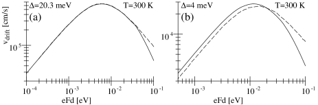
FIG. 4.: Drift-velocity versus field for: (a) strongly coupled SL as in Fig. 1 but $T=300$K. (b) weakly coupled SL with $\Delta=4$ meV, $1/\tau_{\rm imp}=15$ ps^-1, $T=300$K. Full line: NGF calculation. Dashed line: MC-simulation of BTE.

REFERENCES

- [1] C. Jacoboni and L. Reggiani, Rev. Mod. Phys. 55, 645 (1983).
- [2] L. P. Kadanoff and G. Baym, Quantum Statistical Mechanics (Benjamin, New York, 1962); L. V. Keldysh, Sov. Phys. JETP 20, 1018 (1965), [Zh. Eksp. Theor. Fiz. 47, 1515 (1964)].
- [3] G. D. Mahan, Many-Particle Physics (Plenum, New York, 1990).
- [4] H. Haug and A.-P. Jauho, Quantum Kinetics in Transport and Optics of Semiconductors (Springer, Berlin, 1996).
- [5] The recovery of BTE for metals can be made rigorous within the Landau Fermi liquid theory. For semiconductors, however, several additional subtleties must be considered, see, e.g., V. Špička and P. Lipavský, Phys. Rev. Lett. 73, 3439 (1994); V. Špička and P. Lipavský, Phys. Rev. B 52, 14615 (1995).
- [6] L. Reggiani, P. Lugli, and A.-P. Jauho, Phys. Rev. B 36, 6602 (1987); L. Reggiani, L. Rota, and L. Varani, phys. status solidi (b) 204, 306 (1997).
- [7] D. K. Ferry et al., Phys. Rev. Lett. 67, 633 (1991); R. Bertoncini and A.-P. Jauho, Phys. Rev. Lett. 68, 2826 (1992); S. Haas, F. Rossi and T. Kuhn, Phys. Rev. B 53, 12855 (1996).
- [8] Semiconductor Superlattices, Growth and Electronic Properties, edited by H. T. Grahn (World Scientific, Singapore, 1995).
- [9] L. Esaki and R. Tsu, IBM J. Res. Develop. 14, 61 (1970).
- [10] X. L. Lei, N. J. M. Horing, and H. L. Cui, Phys. Rev. Lett. 66, 3277 (1991); A. A. Ignatov, E. P. Dodin, and V. I. Shashkin, Mod. Phys. Lett. B 5, 1087 (1991); R. R. Gerhardts, Phys. Rev. B 48, 9178 (1993).
- [11] R. Tsu and G. Döhler, Phys. Rev. B 12, 680 (1975); S. Rott, N. Linder, and G. H. Döhler, Superlattices and Microstructures 21, 569 (1997).
- [12] R. Aguado et al., Phys. Rev. B 55, 16053 (1997); A. Wacker, Chap. 10 in Theory of transport properties of semiconductor nanostructures, edited by E. Schöll (Chapman and Hall, London, 1998).
- [13] R. A. Suris and B. S. Shchamkhalova, Sov. Phys. Semicond. 18, 738 (1984), [Fiz. Tekh. Poluprovodn. 18, 1178 (1984)].
- [14] V. V. Bryksin and P. Kleinert, J. Phys.: Cond. Mat. 9, 7403 (1997).
- [15] B. Laikhtman and D. Miller, Phys. Rev. B 48, 5395 (1993).
- [16] A. Wacker and A.-P. Jauho, Phys. Rev. Lett. 80, 369 (1998).
- [17] R. Lake and S. Datta, Phys. Rev. B 45, 6670 (1992); R. Lake et al., J. Appl. Phys. 81, 7845 (1997).
- [18] S. Rott et al., Phys. Rev. B 59, 7334 (1999).
- [19] Note that a constant matrix element is equivalent to localized phonons, which is far from realistic. Nevertheless our MC results with this approximation resemble those with the correct matrix elements [20]. Thus our approximations give at least qualitatively good results.
- [20] S. Rott et al., Physica E 2, 511 (1998).