Quasiparticle Band Structure and Density Functional Theory:
Single-Particle Excitations and Band Gaps in Lattice Models

Abstract

We compare the quasiparticle band structure for a model insulator obtained from the fluctuation exchange approximation (FEA) with the eigenvalues of the corresponding density functional theory (DFT) and local density approximation (LDA). The discontinuity in the exchange-correlation potential for this model is small and the FEA and DFT band structures are in good agreement. In contrast to conventional wisdom, the LDA for this model overestimates the size of the band gap. We argue that this is a consequence of an FEA self-energy that is strongly frequency dependent, but essentially local.

PACS numbers: 71.10.-w, 71.15.Mb, 71.10.Fd, 71.45.Gm

I Introduction

Hohenberg and Kohn[1] showed that the total energy of the interacting electron gas in an external potential is given by the minimum of a functional of the electron density, $n({\bf r})$. This seminal result was followed a year later by the Kohn–Sham [2] ‘trick’ which reduces the original problem to an auxiliary problem involving fictitious non-interacting particles moving in a one-body effective potential composed of the external potential, the familiar Hartree potential, and an exchange-correlation potential, $v_{xc}[n]$, which is a universal nonlocal functional of the spatially inhomogeneous density. This innovation, together with local approximations for the exchange-correlation potential (LDA), underlies electronic structure calculations for a wide variety of bulk materials, surfaces, and superlattices. Properties that can be obtained from total energy calculations are generally found to be accurate within a few percent.[3]

A by-product of the Kohn-Sham (KS) approach is a set of single-particle eigenvalues. Without rigorous basis (even for the exact density functional theory), these are often taken to be single-particle excitation energies. This interpretation, together with the LDA, leads to reasonably good agreement with experimentally determined single-particle energies for many materials,[3] but encounters difficulties in numerous other materials ranging from commonplace semiconductors to exotic f-electron intermetallics. Here we report on calculations that explore the relation between quasiparticle energies, eigenvalues obtained from density functional theory (DFT), and those from a corresponding LDA.

Notable among those materials for which LDA eigenvalues do not provide a correct account of single-particle excitation energies are seemingly ordinary insulators such as Si and diamond for which the LDA eigenvalues lead to sizeable underestimates of band gaps. A more dramatic discrepancy occurs for the strongly-correlated heavy-electron materials. For this class of rare-earth and actinide compounds, effective masses obtained from electronic structure calculations in the LDA differ by one to two orders of magnitude from those observed in de Haas van Alphen experiments.[4] Among the ground states exhibited by the heavy-electron materials are insulators characterized by small gaps to low-energy charge excitations, which display experimental signatures of heavy-electron metals upon doping. In contrast to ‘ordinary’ insulators, LDA electronic structure calculations seem to overestimate the size of energy gaps in these ‘Kondo’ insulators as observed[5] for Ce₃Bi₄Pt₃. The insulating parent compounds of the high-temperature superconductors are also examples of materials for which the LDA does not adequately describe electronic correlations; the LDA erroneously predicts that these are metals.[6] In the absence of a rigorous theoretical connection between the eigenvalues of density functional theory and single-particle excitation energies, it has become a matter of debate whether improved approximation to the exchange-correlation potential can remove discrepancies between calculated eigenvalues and observed single-particle excitation energies.

The only rigorous connection[7] between KS eigenvalues and quasiparticle energies is that the eigenvalue of the highest occupied KS wave function is equal to the chemical potential, $\mu$. This result may be used to calculate the band gap of an insulator,[8, 9]

$$E_{g}=E_{cbm}^{N+1}-E_{vbm}^{N},$$ (1)

where $E_{cbm}^{N+1}$ is the KS eigenvalue of the appropriate conduction band minimum calculated for the $N+1$-particle system and $E_{vbm}^{N}$ is the KS eigenvalue of the appropriate valence band maximum for the (insulating) $N$-particle system. Here, any ambiguity in $\mu$ for a semiconductor is removed by taking appropriate limits for an $M$ particle system as $M\rightarrow N+1$ from above and $M\rightarrow N$ from below. The “band gap problem” with the KS eigenvalues[8, 9] appears if the gap is expressed soley in terms of the eigenvalues of the $N$-particle system $E^{N}$,

$$E_{g}=E_{cbm}^{N}-E_{vbm}^{N}+\Delta V_{xc},$$ (2)

where $\Delta V_{xc}$ is a spatially constant discontinuity of the exchange-correlation potential in going from an $N$ particle system with an exactly filled valence band to an $N+1$ particle system with exactly one electron in the conduction band. Because (for a macroscopic solid) the electron densities in these two cases differ by ${\cal O}(1/N)$, $\Delta V_{xc}$ is in a sense maximally nonlocal: it depends on the total electron count (integrated over the entire system) and on the specific periodic structure of the solid.

Insofar as $\Delta V_{xc}$ is small for a particular insulator, the major source of error in a LDA calculation of its gap lies in the approximation for the remaining part of $V_{xc}$, which is taken to be local, possibly with gradient corrections.[10] Otherwise, $\Delta V_{xc}$ must be explicitly included in an $N$ particle LDA calculation for the gap.

There may be no universal solution to these problems; $\Delta V_{xc}$ may be large for one class of systems and small for others, and the physics underlying the contribution of $\Delta V_{xc}$ may also differ from case to case. To address this issue, one needs quasiparticle energies, true DFT eigenvalues, and LDA eigenvalues for the same system. Unfortunately, one or another of these are known exactly in only a few special cases, and there is no even remotely realistic case for which all three are known exactly. Hence, one is always comparing approximate results, and a major concern is whether these comparisons are meaningful.

An essentially exact LDA is known for 3D continuum systems, but in this case neither the true DFT eigenvalues nor the exact quasiparticle energies are known with any reliability. For this case, Godby, Schlüter, and Sham [11] studied semiconductors and tried to obtain meaningful comparisons by working consistently within the GW approximation, which was used to calculate the LDA exchange-correlation potential, quasiparticle energies, and the true exchange-correlation potential for Si, GaAs, and AlAs. They found that the discontinuity in the exchange-correlation potential accounted for much of the underestimate of the band gap in the LDA.

Other groups have worked with 1D model Hamiltonians with a small number of lattice sites, for which essentially exact quantum Monte Carlo calculations are possible.[12, 13] Problems with this approach include the relevance of results from 1D (with its well-known pathologies) to more realistic systems,[14] the lack of accurate quasiparticle energies for comparison, and the question of what constitutes an appropriate LDA for comparison with the exact results.[15] These references find that the discontinuity in the exchange-correlation potential is small,[12] or large.[13]

In the spirit of Godby, Schlüter and Sham,[11] we have studied the DFT, LDA, and quasiparticle energies for a 2D two-band model insulator on a bipartite lattice with Hubbard on-site interactions. In place of the GW approximation we use the fluctuation exchange approximation[16] (FEA), a fully self-consistent conserving approximation,[17] to calculate quasiparticle band structures and the thermodynamic potential. Because we work at finite temperatures, we use Mermin’s finite-temperature generalization[18] of the Hohenberg-Kohn theorems to provide the connection between true DFT and the FEA: we define our “full DFT” to reproduce the site densities of the FEA and we define our LDA for the exchange-correlation potential from the FEA for the single-band Hubbard model, which plays a role analogous to that of the homogeneous interacting electron gas in continuum DFT. We consider model parameters for which no fluctuation channel is strongly dominant, but for which spin fluctuations and fluctuations in the particle-particle channel provide larger contributions to the thermodynamic potential than do density fluctuations.

Calculations for our model insulator show that the FEA band gap is slightly smaller than that for the DFT and that the band gap for the LDA is significantly larger than the FEA gap. These relationships among gaps differ significantly from the conventional electronic structure wisdom. We believe that the relationships we find are a consequence of a strongly frequency-dependent but essentially local self-energy. Our self-energies are calculated using a propagator-renormalized theory in which the bare parameters of the Hamiltonian have been eliminated from thermodynamic potential.[19] This propagator-functional formalism casts the thermodyanmic potential as a functional of observable spectral functions.[20] From this viewpoint, the form of the self-energy is a spectral property with generalizable physical consequences that transcend the specific underlying Hamiltonian. The ubiquitous quasiparticles of Landau’s Fermi liquid theory provide a familiar example. They arise not only in liquid ³He and in metals, but appear also in self-consistent calculations based on Hubbard Hamiltonians in three dimensions. In this spirit, we belive that the effects of the locality and non-locality of the self-energy transcend the underlying Hamiltonians from which they were deduced, and so the essential physics distilled from our results may be applied to the ‘Kondo insulators,’ such as Ce₃Bi₄Pt₃, for which electronic structure calculations in the LDA overestimate band gaps.[5]

In the next section, we introduce single-band and bipartite-lattice Hubbard models and the fluctuation exchange approximation. In Section III the construction of a suitable density functional theory and local density approximation is described. In Section IV, the LDA and FEA are compared. Our conclusions are presented in Section V.

II The Model Insulator

To explore the relation of the eigenvalues of density functional theory to single-particle excitation energies, we take a Hubbard model on a bipartite lattice for our model insulator. The lattice consists of two interpenetrating square (Bravais) lattices, ‘A’ and ‘B;’ an A-site’s nearest neighbors are B-sites and its next nearest neighbors are A-sites. The Hamiltonian for our model is

$$H=\; -\; \sum_{(i,j)\ \sigma}t_{ij}(c^{\dagger}_{i\sigma}c_{j\sigma}+c^{\dagger}_{j\sigma}c_{i\sigma})$$ (4)

$$\;\;\;+\sum_{i\sigma}v_{i}n_{i\sigma}+U\sum_{i}n_{i\uparrow}n_{i\downarrow},$$

where $c_{j\sigma}(c^{\dagger}_{j\sigma})$ annihilates (creates) a particle on site $j$, $t_{ij}$ are hopping matrix elements, $v_{i}$ is an on-site single particle potential that takes the value $v_{A}$ ($v_{B}$) for a site on the A (B) sublattice, and $U$ is the intra-site repulsion experienced by two electrons on the same lattice site. We work in 2D and include nearest-neighbor $t$ and next-nearest-neighbor $t_{xy}$ hopping amplitudes to avoid known pathologies that result from Fermi surface nesting and van Hove singularities at the Fermi surface.

We write the one-body potential for the A (B) sites in the suggestive form $v_{A}=v_{0}-\Delta_{0}$ ($v_{B}=v_{0}+\Delta_{0}$). This potential doubles the unit cell leading to a two-dimensional analog of the Su, Schrieffer, and Heeger Hamiltonian for polyacetylene.[21] For $U=0$, the single-particle excitation energies are

$$E_{\bf k}^{\pm}=\gamma_{\bf k}+v_{0}-\mu\pm\sqrt{|\alpha_{\bf k}|^{2}+\Delta_{0}^{2}},$$ (5)

where

$$\gamma_{\bf k} = -2\;t_{xy}\;(\cos k_{x}+\cos k_{y}),$$ (6)

$$\alpha_{\bf k} = -4\;t\;\cos k_{x}\cos k_{y}e^{i(k_{x}+k_{y})/2}.$$ (7)

For nonzero $U$, the exact solution of this model is unknown. We use the fluctuation exchange approximation (FEA), based on the propagator renormalized perturbation theory of Luttinger and Ward, to provide quasiparticle energies and the basis for constructing full and LDA density functional theories.

The Luttinger and Ward [22] formula expresses the grand thermodynamic potential $\Omega$ as a functional of the fully renormalized Green’s function $G$ and the self energy $\Sigma$,

$$\Omega(T,\mu)=-2\;{\rm Tr}\ [\Sigma G+\ln(-\;G_{0}^{-1}+\Sigma)]+\Phi[G].$$ (8)

Here ‘Tr’ indicates a sum over momentum, frequency, and sublattice arguments,[23] and $G_{0}$ is the Green’s function for the noninteracting system ($U=0$) which contains the bare band structure. When viewed as a functional of $G$ and $\Sigma$, $\Omega$ is stationary with respect to independent variations around the true $G$ and $\Sigma$ for a given $G_{0}$ and $U$, leading to the ‘skeleton diagram’ expansion for the self-energy,

$$\Sigma({\bf k},\varepsilon_{n})=\frac{1}{2}\ \frac{\delta\Phi[G]}{\delta G({\bf k},\varepsilon_{n})},$$ (9)

and to Dyson’s equation,

$$G^{-1}({\bf k},\varepsilon_{n})=G^{-1}_{0}({\bf k},\varepsilon_{n})-\Sigma({\bf k},\varepsilon_{n})\;.$$ (10)

The self-consistent solutions of Eqs. (9) and (10) completely specify $G$ and $\Sigma$, and together with Eq. (8) provide a self-consistent description of single-particle excitation spectra and thermodynamic properties. The FEA entails a specific prescription for $\Phi[G]$ that includes contributions from the exchange of spin, density, and Cooper-pair fluctuations in addition to self-consistent contributions at first (Hartree Fock) and second order in the interaction. The propagator for our model is a $2\times 2$ matrix labeled by sublattice indices; a more detailed discussion of the FEA for the Hubbard model on a bipartite lattice, together with explicit expressions for $\Phi[G]$, appears in the Appendix.

We have solved Eqs. (9) and (10) self-consistently on a $64\times 64$ mesh using a parallel algorithm described elsewhere.[24] This is not our most accurate method for solving the equations of the FEA. The more accurate algorithm of Ref. [26], which does not contain a high-frequency cutoff in the traditional sense, is essential for calculating temperature derivatives of the thermodynamic potential and for performing calculations near an instability to an ordered state. Since none of these conditions apply here, the algorithm of Ref. [24] suffices for our purposes.

The A- and B-site densities needed for the density functional theory calculations described below are obtained directly from the diagonal components of the propagator,

$$n_{i}={2{T}\over{N}}\sum_{{\bf k},n}G_{ii}({\bf k},\varepsilon_{n}),$$ (11)

where $T$ is the temperature and $N$ is the number of ${\bf k}$-points. Because the FEA is a conserving approximation, this is equivalent to calculating the site densities from the thermodynamic potential,

$$n_{i}={{\partial\;\Omega[T,v_{A},v_{B}]}\over{\partial\;v_{i}}}.$$ (12)

Explicit calculations show that this internal self-consistency is achieved to better than $1\%$.

III Density Functional Theory for Lattice Models

Following Mermin,[18] it is straightforward to show that the thermodynamic potential of our model is a stationary function of the A- and B-site densities. The thermodynamic potential (with arguments $T$ and $\mu$ suppressed) is

$$\Omega[\{n_{j}\}]=\Theta[\{n_{j}\}]+\Omega_{H}[\{n_{j}\}]+\Omega_{xc}[\{n_{j}\}]+\Omega_{ext}[\{n_{j}\}],$$ (13)

where $\Omega_{ext}$ is the contribution from the external potential, $\Theta+\Omega_{ext}$ is the grand thermodynamic potential of a system of fictitious non-interacting particles with site densities $\{n_{j}\}$, and $\Omega_{H}$, and $\Omega_{xc}$ are the Hartree and exchange-correlation potential contributions. For our model, the Hartree contribution to $\Omega$ is

$$\Omega_{H}[n_{A},n_{B}]=\frac{1}{4}\;(n_{A}^{2}+n_{B}^{2})\;U,$$ (14)

and the contribution from the external potential $v_{j}$ is

$$\Omega_{ext}[\{n_{j}\}]=\sum_{j}v_{j}n_{j}.$$ (15)

The condition that the grand thermodynamic potential be stationary with respect to variations in the density leads to the set of coupled equations,

$$\frac{d\Theta[\{n_{j}\}]}{dn_{i}}+\frac{d\Omega_{ext}[\{n_{j}\}]}{dn_{i}}+\frac{d\Omega_{H}[\{n_{j}\}]}{dn_{i}}+\frac{d\Omega_{xc}[\{n_{j}\}]}{dn_{i}}=0.$$ (16)

A Full Density Functional Theory

The KS formulation at finite temperature invokes an auxiliary system of noninteracting particles in a one-body effective potential $V_{\rm eff}$, that is defined by writing Eq. (16) in the form,

$$\frac{d\Theta[\{n_{j}\}]}{dn_{i}}+V_{\rm eff}[\{n_{j}\}]=0\;.$$ (17)

The thermodynamic potential for the auxiliary problem is

$$\Omega_{\rm eff}^{0}=-2T\sum_{\alpha}\ln\left[1+e^{-\beta(\epsilon_{\alpha}-\mu)}\right],$$ (18)

where the single-particle eigenvalues $\epsilon_{\alpha}$ satisfy the Schrödinger equation

$$(K+V_{\rm eff}[\{n_{j}\}])\;\psi_{\alpha}=\epsilon_{\alpha}\psi_{\alpha}\;,$$ (19)

and $K$ is the hopping Hamiltonian (first term of Eq. (4)). The site densities at finite temperature are related to the KS wave functions through

$$n_{i}=2\sum_{\alpha}\;|\psi_{\alpha}({\bf r}_{i})|^{2}f(\epsilon_{\alpha}),$$ (20)

where $f(\epsilon)$ is the usual Fermi function. Because Eq. (17) is also the KS variational condition for the auxiliary problem with $V_{eff}$ regarded as an external potential, densities that result from the self-consistent solution of Eqs. (19) and (20) are guaranteed to be identical to those of the original interacting system.

For our model, $V_{xc}[\{n_{j}\}]$ is unknown; we use the FEA site densities together with the KS formulation to find the exchange correlation potential, $V_{xc}=(v^{A}_{xc},v^{B}_{xc})$. To do this, we find one body potentials $v^{A}_{\rm eff}$ and $v^{B}_{\rm eff}$, for which the site-densities of the finite-temperature auxiliary KS problem are the same as the FEA site-densities, and invert the definition of $V_{\rm eff}$ to obtain $V_{xc}$. A convenient expression (equivalent to Eq. (20)) for the site-densities of the non-interacting problem is obtained by taking the trace of the site-diagonal components of the propagator for the non-interacting system given in Eq. (30). The full DFT band structure can be extracted from Eqs. (5) using $v_{i}=v^{i}_{\rm eff}$.

Because the FEA is a conserving approximation, the FEA grand thermodynamic potential has the same stationary properties with respect to variations of $G$ and $\Sigma$ as the exact grand thermodynamic potential. As a consequence, the exchange-correlation potential that we have calculated is identical to that calculated from Sham’s integral equation[25] for $V_{xc}$.

B The Local Density Approximation

For our model, the single-band Hubbard model plays the role analogous to that of the uniform interacting electron gas in the formulation of the continuum LDA for electronic structure theory. So, we use Eq. (13) to calculate $\Omega_{xc}[n]$ in the FEA for the single-band Hubbard model (the Hamiltonian of Eq. 4 with $v_{i}=0$) with the same “Coulomb potential,” $U$. To avoid possible confusion, we emphasize that in this case the electron density is the same at every site, and $\Omega_{xc}$ becomes a simple function of the uniform density, $n$. This entails evaluating Eq. (8) with the self-consistently calculated FEA propagator for the single-band Hubbard model, evaluating the Hartree contribution to the thermodynamic potential, and rearranging Eq. (13) with $\Omega_{ext}=0$ to extract $\Omega_{xc}$. The LDA exchange-correlation potential is

$$V_{xc}^{LDA}(n)=\frac{d\Omega_{xc}(n)}{dn}.$$ (21)

In this way the LDA exchange-correlation potential corresponding to the full DFT is calculated in an approximation equivalent to that of the FEA calculation.

Given $V_{xc}^{LDA}(n)$, Eqs. (19) and (20) can be solved directly with external potentials $v_{0}$ and $\Delta_{0}$, subject to the constraint that the total density agrees with that of the FEA calculation. As in the case of the DFT, Eqs. (5) with the potentials $v^{LDA}_{i,\;{\rm eff}}$ determine the LDA band structure.

IV Results

We focus on single-band and two-band models with next-nearest-neighbor hopping matrix element $t_{xy}=0.35$ and $U=3$. This set of parameters avoids possible complications of dominant fluctuation contributions in any one specific channel as might arise as a consequence of, for example, Fermi surface nesting.[27] For the model insulator (see below), the contributions to the grand thermodynamic potential from the Hartree and second-order diagrams are the largest. Somewhat smaller spin, density, and Cooper pair fluctuation contributions are all roughly the same order. For $T=0.02$, explicit values for the $\Phi$-functionals in their respective channels are: $\Phi_{2}=-1.87\times 10^{-2}$, $\Phi_{\rm pp}=5.06\times 10^{-3}$, $\Phi^{df}_{ph}=8.41\times 10^{-4}$, and $\Phi^{sf}_{ph}=-3.31\times 10^{-3}$.

The exchange-correlation contribution to the thermodynamic potential $\Omega_{xc}$ as a function of density for a single-band Hubbard model with next-nearest-neighbor hopping matrix element $t_{xy}=0.35$, $U=3$ and $T=0.08$ is shown in Fig. 1 (we henceforth measure energies in units of the nearest-neighbor hopping matrix element $t$).

FIG. 1.: The exchange-correlation contribution to the thermodynamic potential $\Omega_{xc}$ as a function of density for the single-band Hubbard model in the fluctuation exchange approximation (FEA) for $U=3$ at two temperatures. The solid line is a fit to 77 points (see text) for $T=0.08$. The widely spaced points are calculated for $T=0.02$.

The solid line is a polynomial fit of the form,

$$\Omega_{xc}(n)=\sum_{i=2}^{10}a_{i}n^{i}$$ (22)

through 77 data points. The coefficients, presented in Table 1, lead to a fit with an error of less than $1\%$ over the entire density range; the worst agreement occurring at low density.

TABLE I.: Values of the coefficients $a_{i}$ in Eq. (22) for the exchange-correlation contribution to the grand thermodynamic potential as a function of density. These parameters are for $U=3$, $T=0.08$, and $t_{xy}=0.35$.

$a_{2}$ = -1.32532	$a_{3}$ = -0.300919	$a_{4}$ = 3.27475
$a_{5}$ = -13.7277	$a_{6}$ = 29.0402	$a_{7}$ = -34.1589
$a_{8}$ = 21.9011	$a_{9}$ = -7.11752	$a_{10}$ = 0.917821

It is interesting to note, in contrast to the exchange-correlation energy used in by Ref. [12], that there is no evidence for a significant $n^{4/3}$ contribution to $\Omega_{xc}$.[27] Fig. 1 also shows $\Omega_{xc}(n)$ for $T=0.02$ at several densities, from which we conclude that $\Omega_{xc}(n)$ is weakly temperature dependent over the range $0.02<T<0.08$. The function $\Omega_{xc}(n)$ is to a reasonable approximation linear in $U$ (see Fig. 2); the largest deviations occur at high density as might be expected. We calculate the local density approximation of the exchange correlation potential from Eq. (22).

FIG. 2.: The exchange-correlation contribution to the thermodynamic potential $\Omega_{xc}(n)$ for $U=3$ (solid line; see previous figure and text), $U=1$ ($\blacksquare$), and the $U=1$ result scaled by a factor of 3 ($\blacktriangle$).

We now compare the FEA single-particle excitations of an insulator to the eigenvalues obtained from the full DFT and those from the LDA. To this end we calculate the fully self-consistent self-energy in the FEA for a bare[28] staggered potential $\Delta_{0}=2.532$. The quasiparticle band structure is obtained from the zeros of the real part of the denominator of the retarded Green’s function $G^{\rm R}$. The fully renormalized retarded propagator was constructed using Dyson’s equation and the retarded self-energy. The latter was obtained from an analytic continuation of the self-energy from the imaginary-frequency axis to the real-frequency axis using N-point Padé Approximants.[29] The resulting band structure for $\Delta_{0}=2.532$ and $n=1.000$ (with $n_{A}^{FEA}=1.688$ and $n_{B}^{FEA}=0.312$), shown in Fig. 3 for ${\bf k}$ along the high-symmetry path $\Gamma-X-M-\Gamma$ in the square zone, is that of an insulator with an indirect gap $E_{g}=E_{X}^{+}-E_{M}^{-}=1.318$. The corresponding full DFT band structure is found by evaluating the (bare) dispersion relations in Eq. (5) using on-site one body potentials $v,\Delta$ for which the site densities $n_{A}$ and $n_{b}$ are equal to $n_{A}^{FEA}$ and $n_{B}^{FEA}$. Starting from the (renormalized) on-site single-body potentials of the FEA $(v^{FEA},\Delta^{FEA})$, a Newton-Raphson method allowed us to determine (to 1 part in $10^{8}$) $v^{DFT}=-0.745$ and $\Delta^{DFT}=1.368$. The DFT band structure appears in comparison with that for the FEA in Fig. 3. The fact that these band structures are essentially indistinguishable suggests that the discontinuity in the exchange-correlation potential is small. In Fig. 4 we show the ‘exact’ $V_{xc}^{FEA}(n)$ obtained from $v^{DFT}$ and $\Delta^{DFT}$ for a range of densities about $n=1$ and observe that, as expected, $V_{xc}^{A}$ and $V_{xc}^{B}$ each show a small discontinuity $|\Delta V_{xc}|=0.026$. Note that the small structure appearing at the high-density side ($n=1.00^{+}$) of the discontinuity is not physically significant, but is rather a numerical artifact reflecting a finite high-frequency cutoff in the FEA calculation; this feature is systematically reduced as the number of Matsubara frequencies kept in the calculation is increased.[30]

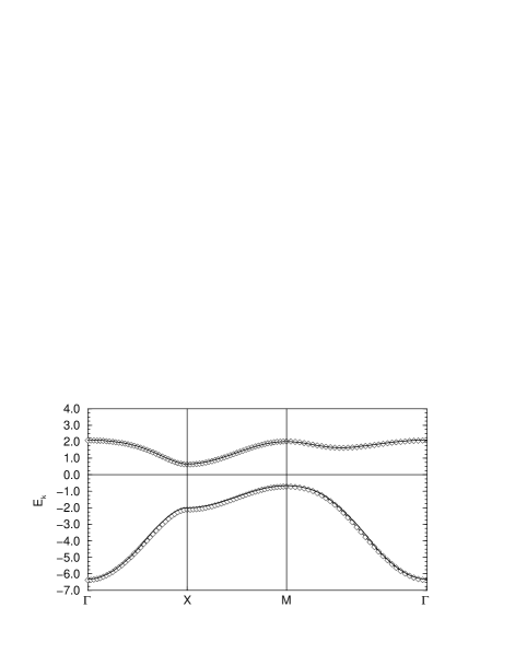
FIG. 3.: The band structure for ${\bf k}$ along high symmetry directions in the Brillouin zone from the FEA calculation (solid) compared with that from the DFT ($\diamond$) for $T=0.08$, $U=3$, and $t_{xy}=0.35$.

To calculate the band structure in the LDA, we take $V_{xc}^{LDA}$ from Eqs. (21) and (22), and solve Eqs. (19) and (20) using a Newton-Raphson method to find on-site one-body potentials $(v^{LDA},\Delta^{LDA})$ that yield the same total density with the same bare staggered potential $\Delta_{0}$ as in the FEA calculation. The LDA band structure obtained from Eqs. (5) with $(v^{LDA},\Delta^{LDA})$ is shown compared with that for the FEA in Fig. 5. For $n\approx 1$, $\partial n/\partial\mu$ is vanishingly small and a wide range of $v^{LDA}$ lead to a $\Delta_{0}$ and $n$ equal to those of the FEA calculation. On the other hand, $\Delta^{LDA}$ is determined to high accuracy by our procedure and is largely insensitive to changes in $v^{LDA}$ for $n\sim 1$. Since $T$ is much smaller than the (indirect) band gap resulting from $\Delta^{LDA}$, we take $v^{LDA}$ so that the chemical potential lies in the middle of the gap as expected on physical grounds. We have explicitly verified that this choice leads to $n=n^{FEA}$ and $\Delta_{0}=\Delta_{0}^{FEA}$ to within the accuracy to which these quantities are known.

The LDA and FEA band structures differ significantly; the LDA band structure cannot be corrected by uniformly and independently shifting the bands by a constant amount. The LDA band structure cannot be corrected by using the “scissors operator.” An examination of the spatial dependence of the FEA self-energy shows that the $\Sigma_{ij}$ are essentially local. The self-energy is essentially uniform in $\bf{k}$ and strongly frequency dependent. The excitation energies $E_{k}$ are the poles of the retarded propagator, $G^{R}$. By combining the appropriate analytic continuation of Eq. (30) with Dyson’s equation, we express $G^{R}$ in terms of the components of the self-energy and find that the poles of $G^{R}$ satisfy

$$\left[E_{\bf k}+\Delta_{0}+\mu+\gamma_{\bf k}-\Sigma_{AA}(E_{\bf k})\right]\times$$ (23)

$$\;\;\;\left[E_{\bf k}+\Delta_{0}+\mu+\gamma_{\bf k}-\Sigma_{BB}(E_{\bf k})\right]-$$ (24)

$$\;\;\;\left[\alpha_{\bf k}+\Sigma_{AB}(E_{\bf k})\right]\left[\alpha^{*}_{\bf k}+\Sigma_{BA}(E_{\bf k})\right] = 0.$$ (25)

Here $\alpha_{\bf k}$ and $\gamma_{\bf k}$ are defined as in Eq. (7) and we have used $\Sigma_{ij}({\bf k},\varepsilon)\sim\Sigma_{ij}(\varepsilon)$. The $E_{\bf k}$ that solves Eq. (25) has a ${\bf k}$-dependence that not only reflects of that of $\gamma_{\bf k}$ and $\alpha_{\bf k}$ but also includes implicit additional ${\bf k}$-dependence through the frequency dependence of the $\Sigma_{ij}$.

FIG. 4.: The ‘exact’ exchange-correlation potential $V_{xc}$ (see text) for A-($\bullet$) and B-sites($\triangle$). The discontinuity is $\sim 0.02$ and occurs at half filling.

As is plainly evident from Fig. 5, the LDA overestimates the the band gap by about a factor of 3. In the light of LDA calculations for insulators, the result $E_{g}^{LDA}>E_{g}^{FEA}$ is perhaps surprising. Since the FEA and the self-consistent GW approximation can be viewed as propagator-functional theories, physical properties may be viewed as a consequence of the form of spectral functions[19] rather than of the form of a particular Hamiltonian. Considered in this way, results of continuum calculations are relevant insofar as they lead to trends in self-energies and hence spectral functions. From this perspective, we believe that the explanation for our results lies in the work of Godby, Schlüter, and Sham.[11] They observed that, for the GW approximation, the nonlocality of the self-energy tends to a widen the gap while frequency dependence tends to narrow the gap. Given the importance of the frequency dependence of $\Sigma_{ij}$ in determining the FEA band structure and given that the DFT band structure is obtained from dispersion relations for a non-interacting system, albeit with largely ‘renormalized’ on-site potentials, the observed close agreement between these band structures may be of a rather subtle physical origin. This agreement may also be in part a reflection of a moderate interaction strength ($U\sim 3/8$ of the bare, $\Delta_{0}=0$, bandwidth) and may degrade with larger $U$. It is also evident from the DFT calculation (see Fig. 4) that $V_{xc}^{A}$ and $V_{xc}^{B}$ are of opposite sign for the density range in which we are working. On the other hand, $\Omega_{xc}$ of Fig. 1 leads to a $V_{xc}^{LDA}<0$ over the entire density range. To compensate, the LDA must increase the size of $\Delta^{LDA}$, which increases the gap.

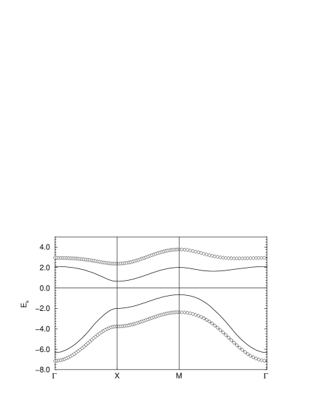
FIG. 5.: A comparison of the FEA band structure (solid) with that of the LDA ($\diamond$), where the LDA is adjusted to yield the same bare staggered field and total density of the FEA calculation.

V Conclusions

We have calculated the renormalized band structure and site densities for a model insulator in the fluctuation exchange approximation (FEA) and in corresponding full and approximate (LDA) density functional theories. The band structures calculated from the full density-functional theory are in good agreement with the ‘true’ band structures obtained from the poles of the retarded FEA propagator. The gap obtained from the DFT is slightly smaller than that of the FEA; the difference is accounted for by a discontinuity in $V_{xc}$ that is small in magnitude. It is also of opposite sign to that observed in GW calculations for ‘real’ ordinary insulators. We find that gap in the LDA is larger than that of the full DFT. The relationship among the gaps differs from that observed in continuum GW calculations for ordinary insulators. An examination of the FEA self-energy shows it to be essentially local, suggesting that this is a consequence of the frequency dependence of the self-energy. We speculate that such a relationship ought to be observed in the ‘Kondo’ insulators where it is expected that, owing to strong electronic correlations, the frequency dependence of the self-energy is more important than its spatial nonlocality.

The FEA for a Hubbard Model on a Bipartite Lattice

The single-particle propagator is central to the calculation of the density and single-particle excitation spectra. It is convenient to adopt a matrix notation for the propagator in imaginary time for the Hamiltonian in Eq. (4),

$${\cal G}_{ij}({\bf r}_{i}-{\bf r}^{\prime}_{j},\tau)=-<{\cal T}\{\psi({\bf r}_{i},\tau)\psi^{\dagger}({\bf r}_{j}^{\prime},0)\}>\;,$$ (26)

where ${\cal T}$ is the usual Wick’s time ordering operator and $\psi({\bf r}_{i})$ is an annihilation operator acting at ${\bf r}_{i}$, where $i$ is a sublattice index ($i=A,B$). Because of the translational invariance of the full Bravais lattice, the propagator is a function of a coordinate difference. Unlike ${\cal G}_{AA}$, ${\cal G}_{AB}$ is defined on a Bravais lattice that does not include the origin. We find it convenient for numerical calculations on parallel computers to introduce a propagator $G_{ij}$ defined so that $G_{ii}={\cal G}_{ii}$, $G_{AB}({\bf r},\tau)={\cal G}_{AB}({\bf r}-\hat{c},\tau)$, and $G_{BA}({\bf r},\tau)={\cal G}_{BA}({\bf r}+\hat{c},\tau)$, where $\hat{c}$ is a vector that joins a point on the A sublattice to one on the B sublattice. By this definition, the arguments of all components of the propagator range over the same (sub)lattice and the usual Fourier transform connects (${\bf r},\tau$) space to (${\bf k}$, $\varepsilon_{n}$) for all components of $G_{ij}$.

Dyson’s equation (Eq. (10)) should now be interpreted as an equation for the ($2\times 2$) matrices $G$, $G_{0}$ and $\Sigma$. Keeping only nearest-neighbor and next-nearest-neighbor hopping amplitudes, the propagator for the noninteracting system in (${\bf k}$, $\varepsilon_{n}$) space is,

$$G_{0}^{-1}({\bf k},\varepsilon_{n})=$$ (27)

$$\;\;\;\;\;\;\;\;\left(\begin{array}[]{cc}i\varepsilon_{n}-\bar{\gamma}_{\bf k}+\Delta_{0}&-\alpha_{\bf k}\\ -\alpha_{\bf k}^{*}&i\varepsilon_{n}-\bar{\gamma}_{\bf k}-\Delta_{0}\\ \end{array}\right)\;,$$ (30)

where $\bar{\gamma}_{\bf k}=\gamma_{\bf k}+v-\mu$, and $\gamma_{\bf k}$ and $\alpha_{\bf k}$ defined as in Eq. (7) above.

The FEA[16] takes $\Phi[\{G_{ij}\}]$ to be the sum of the Hartree-Fock diagram, the single second-order diagram, and particle-hole and particle–particle bubble chains that describe exchanged density, spin-density, and (singlet) pair fluctuations. For the bipartite lattice, explicit expressions for $\Phi[\{G_{ij}\}]$ are

$$\Phi_{2}\;\, = \;-\frac{1}{/}2{\rm Tr}\left[(\chi^{ph}_{AA})^{2}+(\chi^{ph}_{BB})^{2}+2\chi^{ph}_{AB}\chi^{ph}_{BA}\right]$$ (31)

$$\Phi_{ph}^{df} = \;\frac{1}{/}4{\rm Tr}\{\ln((1+\chi^{ph}_{AA})(1+\chi^{ph}_{BB})-\chi^{ph}_{AB}\chi^{ph}_{BA})$$ (34)

$$-\chi^{ph}_{AA}-\chi^{ph}_{BB}$$

$$+\frac{1}{/}2\left[(\chi^{ph}_{AA})^{2}+(\chi^{ph}_{BB})^{2}\right]+\chi^{ph}_{AB}\chi^{ph}_{BA}\}$$

$$\Phi_{ph}^{sf} = \;\frac{3}{/}4{\rm Tr}\{\ln((1-\chi^{ph}_{AA})(1-\chi^{ph}_{BB})-\chi^{ph}_{AB}\chi^{ph}_{BA})$$ (37)

$$+\chi^{ph}_{AA}+\chi^{ph}_{BB}$$

$$+\frac{1}{/}2\left[(\chi^{ph}_{AA})^{2}+(\chi^{ph}_{BB})^{2}\right]+\chi^{ph}_{AB}\chi^{ph}_{BA}\}$$

$$\Phi_{pp} = \;\frac{1}{/}4{\rm Tr}\{\ln((1+\chi^{pp}_{AA})(1+\chi^{pp}_{BB})-\chi^{pp}_{AB}\chi^{pp}_{BA})$$ (40)

$$-\chi^{pp}_{AA}-\chi^{pp}_{BB}$$

$$+\frac{1}{/}2\left[(\chi^{pp}_{AA})^{2}+(\chi^{pp}_{BB})^{2}\right]+\chi^{pp}_{AB}\chi^{pp}_{BA}\}.$$

Here $\chi^{ph}_{ij}$ and $\chi^{pp}_{ij}$ are particle-hole and particle-particle susceptibility bubbles connecting lattice sites $i$ and $j$ and are related to the fully renormalized Green’s function by

$$\chi^{pp}_{ij}( {\bf q}, \omega_{m})=U(T/N)$$ (42)

$$\sum_{\bf k}\sum_{n}G_{ij}({\bf k}+{\bf q},\varepsilon_{n}+\omega_{m})G_{ji}(-{\bf k},-\varepsilon_{n})$$

$$\chi^{ph}_{ij}( {\bf q}, \omega_{m})=-U(T/N)$$ (44)

$$\sum_{\bf k}\sum_{n}G_{ij}({\bf k}+{\bf q},\varepsilon_{n}+\omega_{m})G_{ji}({\bf k},\varepsilon_{n}).$$

The components of the self-energy matrix are obtained from Eq. (9),

$$\Sigma_{ij}({\bf k},\varepsilon_{n})=\frac{1}{2}\ \frac{\delta\Phi[G]}{\delta G_{ji}({\bf k},\varepsilon_{n})}.$$ (45)

REFERENCES

- [1] P. Hohenberg and W. Kohn, Phys. Rev. 136, B 864 (1964).
- [2] W. Kohn and L. J. Sham, Phys. Rev. 140, A1133 (1965).
- [3] R. O. Jones and O. Gunnarsson, Rev. Mod. Phys. 61, 689 (1989).
- [4] D.W. Hess, P.S. Riseborough, and J.L. Smith, in Encyclopedia of Applied Physics, Vol. 7, edited by G. Trigg (VCH Publishers, New York) 1994.
- [5] K. Takegahara, H. Harima, Y. Kaneta, A. Yanase, J. Phys. Soc. Jap. 62, 2103 (1993).
- [6] W.E. Pickett, H. Krakauer, R.E. Cohen, and D.J. Singh, Science 255, 46 (1992).
- [7] L. J. Sham and W. Kohn, Phys. Rev. 145, 561 (1966).
- [8] L. J. Sham and M. Schlüter, Phys. Rev. Lett. 51, 1888 (1983); L. J. Sham and M. Schlüter, Phys. Rev. B 32, 3883 (1985).
- [9] J. P. Perdew and M. Levy, Phys. Rev. Lett. 51, 1884 (1983).
- [10] J. P. Perdew, K. Burke, Y. Wang, Phys. Rev. B 54, 16533 (1996).
- [11] R. W. Godby, M. Schlüter and L. J. Sham, Phys. Rev. B 37, 10159 (1988).
- [12] O. Gunnarsson and K. Schönhammer, Phys. Rev. Lett. 56, 1968 (1986).
- [13] W. Knorr and R.W. Godby, Phys. Rev. Lett. 68, 639 (1992).
- [14] See e.g., H.J. Shulz, Int. J. Mod. Phys. B 5, 57 (1991).
- [15] L.J. Sham and M. Schlüter, Phys. Rev. Lett. 60, 1582 (1988).
- [16] N.E. Bickers, D.J. Scalapino and S.R. White, Phys. Rev. Lett. 62, 961 (1989).
- [17] G. Baym Phys. Rev. 127, 1391 (1962).
- [18] N.D. Mermin, Phys. Rev. 137, A1441 (1965).
- [19] C. De Dominicis and P.C. Martin, J. Math. Phys. 5, 14 (1964).
- [20] Our calculations here are based on an explicit realization of this systematic program at the single-particle level (mass renormalization).
- [21] W.P. Su, J.R. Schrieffer, and A.J. Heeger, Phys. Rev. Lett. 42, 1698 (1979).
- [22] J.M. Luttinger and J.C. Ward, Phys. Rev. 118, 1417 (1960).
- [23] Here we consider only paramagnetic systems.
- [24] J.W. Serene and D.W. Hess, in Recent Progress in Many-Body Theories, Vol. 3, edited by T.L. Ainsworth et al. (Plenum, New York, 1992); J.W. Serene and D.W. Hess, Phys. Rev. B 44, 3391 (1991).
- [25] L.J. Sham, Phys. Rev. 32, 3876 (1985).
- [26] J.J. Deisz, D.W. Hess and J.W. Serene, in Recent Progress in Many-Body Theories, Vol. 4, edited by E. Schachinger, et al. (Plenum, New York, 1995).
- [27] We note that for n-n hopping only has a similar form, suggesting that is weakly dependent on . This is due largely to the small size of contributions to obtained from the functionals , and () as compared to the contributions from the Hartree term ( for ) and from . We discuss elsewhere the effects of nesting and van Hove singularities on the exchange-correlation functional for 2D systems. For a discussion of the effect of these pathologies on the single particle excitation spectrum in the FEA, see Ref. [24] and J.J. Deisz, D.W. Hess and J.W. Serene, Phys. Rev. Lett. 76, 1312 (1996).
- [28] Here we use ‘bare’ to indicate values that appear (or are trivially related to those that appear) in the Hamiltonian, in contrast to the renormalized single body potentials into which the Hartree contribution to the self-energy has been included.
- [29] H.J. Vidberg and J.W. Serene, J. Low Temp. Phys. 19, 179 (1977).
- [30] We used 256 Matsubara frequencies to calculate for the one-band Hubbard model and have explicitly verified that our LDA is insensitive to any further increases in the high-frequency cutoff.