Possible Spin-Singlet Superconductivity in (TMTSF)₂X: Superconducting Transition Temperature in a Magnetic Field

It is known that the spin-singlet superconductivity is destroyed by both the orbital frustration and the Pauli paramagnetic effect. Recently, the reentrance of the superconductivity which is caused by quantum effect of orbital motions along the open Fermi surfaces in a strong magnetic field has attracted interest .${}^{\hbox{\immediate{\bf{?}},\penalty 1000\hskip 0.91003pt plus 0.70004pt minus 0.70004pt{\bf{?}},\penalty 1000\hskip 0.91003pt plus 0.70004pt minus 0.70004pt{\bf{?}},\penalty 1000\hskip 0.91003pt plus 0.70004pt minus 0.70004pt{\bf{?}},\penalty 1000\hskip 0.91003pt plus 0.70004pt minus 0.70004pt{\bf{?}},\penalty 1000\hskip 0.91003pt plus 0.70004pt minus 0.70004pt{\bf{?}},\penalty 1000\hskip 0.91003pt plus 0.70004pt minus 0.70004pt{\bf{?}})}}$ The anomaly of the resistivity in a strong magnetic field has been observed ${}^{\hbox{\immediate{\bf{?}},\penalty 1000\hskip 0.91003pt plus 0.70004pt minus 0.70004pt{\bf{?}},\penalty 1000\hskip 0.91003pt plus 0.70004pt minus 0.70004pt{\bf{?}})}}$ in quasi-one-dimensional (Q1D) organic superconductors (TMTSF)₂X (where anion X is ClO₄ or PF₆) when the magnetic field is applied along the second conducting axis ($b$ axis). This is thought to be a signal of the superconductivity in a strong magnetic field, since the critical temperature $T_{\rm c}(H)$ exceeds both the upper critical field $H_{\rm c2}$ derived in GL theory ${}^{\hbox{\immediate{\bf{?}},\penalty 1000\hskip 0.91003pt plus 0.70004pt minus 0.70004pt{\bf{?}})}}$ and Pauli paramagnetic limit $H_{\rm P}$[T]$=1.84T_{\rm c}$[K] .${}^{\hbox{\immediate{\bf{?}},\penalty 1000\hskip 0.91003pt plus 0.70004pt minus 0.70004pt{\bf{?}})}}$

In the Q1D system, it has been known ${}^{\hbox{\immediate{?},\penalty 1000\hskip 0.91003pt plus 0.70004pt minus 0.70004pt{?},\penalty 1000\hskip 0.91003pt plus 0.70004pt minus 0.70004pt{?},\penalty 1000\hskip 0.91003pt plus 0.70004pt minus 0.70004pt{?},\penalty 1000\hskip 0.91003pt plus 0.70004pt minus 0.70004pt{?},\penalty 1000\hskip 0.91003pt plus 0.70004pt minus 0.70004pt{?})}}$ that the spin-singlet superconductivity is not destroyed completely due to the Zeeman effect by constructing the Larkin-Ovchinnikov-Fulde-Ferrell (LOFF) superconducting state ${}^{\hbox{\immediate{\bf{?}},\penalty 1000\hskip 0.91003pt plus 0.70004pt minus 0.70004pt{\bf{?}})}}$ in which Cooper pair is formed by the electrons $({\mbox{\boldmath$k$}},\uparrow)$ and $(-{\mbox{\boldmath$k$}}+{\mbox{\boldmath$q$}},\downarrow)$. The electron $(-{\mbox{\boldmath$k$}}+{\mbox{\boldmath$q$}},\downarrow)$ can be on the down-spin Fermi surface for any $({\mbox{\boldmath$k$}},\uparrow)$ on the up-spin Fermi surface in a 1D system by choosing the appropriate $q$, which is similar to the nesting of the Fermi surface in the spin-density-wave (SDW) case. Even in the Q1D system, the “nesting” condition for the LOFF state was thought to become perfect in the strong magnetic field .${}^{\hbox{\immediate{?},\penalty 1000\hskip 0.91003pt plus 0.70004pt minus 0.70004pt{?},\penalty 1000\hskip 0.91003pt plus 0.70004pt minus 0.70004pt{?},\penalty 1000\hskip 0.91003pt plus 0.70004pt minus 0.70004pt{?},\penalty 1000\hskip 0.91003pt plus 0.70004pt minus 0.70004pt{?},\penalty 1000\hskip 0.91003pt plus 0.70004pt minus 0.70004pt{?},\penalty 1000\hskip 0.91003pt plus 0.70004pt minus 0.70004pt{?})}}$ These theoretical calculations ${}^{\hbox{\immediate{?},\penalty 1000\hskip 0.91003pt plus 0.70004pt minus 0.70004pt{?},\penalty 1000\hskip 0.91003pt plus 0.70004pt minus 0.70004pt{?},\penalty 1000\hskip 0.91003pt plus 0.70004pt minus 0.70004pt{?},\penalty 1000\hskip 0.91003pt plus 0.70004pt minus 0.70004pt{?},\penalty 1000\hskip 0.91003pt plus 0.70004pt minus 0.70004pt{?},\penalty 1000\hskip 0.91003pt plus 0.70004pt minus 0.70004pt{?})}}$ for $T_{\rm c}(H)$ based on the approximation that the Fermi velocity is independent of the position of the Fermi surface.

Recently, Lebed ${}^{\hbox{\immediate{\bf{?}})}}$ has shown that the nonlinearity effect of the energy dispersion along the $a$ axis on the Zeeman splitting causes the finite upper critical field in Q1D systems. He obtained that the critical magnetic field for the LOFF state is $H^{\rm LOFF}_{\rm P}\sim 0.6\sqrt{t_{a}/t_{b}}H_{\rm P}$, where $t_{a}$ and $t_{b}$ are the hopping matrix elements along $a$ and $b$ axes, respectively. Applying this result to (TMTSF)₂X, $H^{\rm LOFF}_{\rm P}\sim 4$Tesla is obtained, which is smaller than the experimentally observed value by Lee et al. (at least $7$T) .${}^{\hbox{\immediate{?},\penalty 1000\hskip 0.91003pt plus 0.70004pt minus 0.70004pt{?})}}$ This result may suggest that the superconductivity in this system is a spin-triplet state which is not affected by the Zeeman effect. However, $T_{\rm c}(H)$ measured by Lee et al. does not reveal the reentrant behavior expected in the case of spin-triplet superconductivity. ${}^{\hbox{\immediate{?},\penalty 1000\hskip 0.91003pt plus 0.70004pt minus 0.70004pt{?},\penalty 1000\hskip 0.91003pt plus 0.70004pt minus 0.70004pt{?},\penalty 1000\hskip 0.91003pt plus 0.70004pt minus 0.70004pt{?},\penalty 1000\hskip 0.91003pt plus 0.70004pt minus 0.70004pt{?})}}$

In this paper, we study $T_{\rm c}(H)$ of a Q1D spin-singlet superconductor by taking the optimal pair momentum $q$ and introducing the higher harmonic terms along the second conducting axis in the tight-binding model, which has been discussed in the field-induced-spin-density-wave (FISDW) ${}^{\hbox{\immediate{\bf{?}},\penalty 1000\hskip 0.91003pt plus 0.70004pt minus 0.70004pt{\bf{?}},\penalty 1000\hskip 0.91003pt plus 0.70004pt minus 0.70004pt{\bf{?}})}}$ and the quantum hole effect (QHE) ${}^{\hbox{\immediate{\bf{?}},\penalty 1000\hskip 0.91003pt plus 0.70004pt minus 0.70004pt{\bf{?}})}}$ in FISDW. We consider both isotropic and anisotropic pairing states for spin-singlet superconductivity, since the symmetry of the pairing is still controversial .${}^{\hbox{\immediate{\bf{?}},\penalty 1000\hskip 0.91003pt plus 0.70004pt minus 0.70004pt{\bf{?}})}}$

We consider the anisotropic tight-binding model including the effect of the Zeeman splitting (we take $\hbar=k_{\rm B}=c_{0}=1$, where $c_{0}$ is the velocity of light):

$$E_{{\mbox{\boldmath$k$}},\sigma} = -2t_{a}\cos(ak_{x})-2t_{b}\cos(bk_{y})-2t_{2b}\cos(2bk_{y})$$ (1)

$$-2t_{3b}\cos(3bk_{y})-2t_{4b}\cos(4bk_{y})-2t_{c}\cos(ck_{z})$$

$$-\sigma\mu_{\rm B}H-\mu,$$

where $t_{a}\gg t_{b}\gg|t_{2b}|>|t_{3b}|>|t_{4b}|\sim t_{c}$, $\sigma\mu_{\rm B}H$ is the Zeeman energy for $\uparrow(\downarrow)$ spin $(\sigma=+(-))$ and $\mu$ is the chemical potential to give the quarter filled electrons.

The orbital effect of the magnetic field is treated by the Peierls substitution, i.e. ${\cal H}_{0}=E({\mbox{\boldmath$k$}}\rightarrow-i\nabla-e{\mbox{\boldmath$A$}})$. We take the vector potential $A$ as ${\mbox{\boldmath$A$}}=(0,0,-Hx)$. Since $t_{a}\gg t_{b}$, we can linearize the energy dispersion along $k_{x}$ for each $k_{y}$. Then the eigenvalues are given by

$$\epsilon^{\alpha}_{k_{x},k_{y},\sigma}=v^{\rm F}_{k_{y},\sigma}(\alpha k_{x}-k^{\rm F}_{k_{y},\sigma}),$$ (2)

where $\alpha={\rm sgn}(k_{x})$ refers to the right/left sheet of the Fermi surface. Although we linearize the dispersion, we consider the $k_{y}$ and $\sigma$ dependence of the Fermi wave number $k^{\rm F}_{k_{y},\sigma}$ and the Fermi velocity along the $a$ axis, $v^{\rm F}_{k_{y},\sigma}=2t_{a}a\sin(ak^{\rm F}_{k_{y},\sigma})$. Note that $k^{\rm F}_{k_{y},\sigma}$ and $v^{\rm F}_{k_{y},\sigma}$ do not depend on $k_{z}$ when the magnetic field is applied along the $b$ axis. For given $k_{y}$ and $\sigma$, $k^{\rm F}_{k_{y},\sigma}$ is obtained by,

$$k^{\rm F}_{k_{y},\sigma} = \frac{1}{a}\cos^{-1}\left[(2t_{b}\cos(bk_{y})+2t_{2b}\cos(2bk_{y})\right.$$ (3)

$$+ 2t_{3b}\cos(3bk_{y})+2t_{4b}\cos(4bk_{y})$$

$$+ \left.\sigma\mu_{\rm B}H+\mu)/t_{a}\right].$$

The corresponding eigenstates are

$$\phi^{\alpha}_{{\mbox{\boldmath$k$}},\sigma}({\mbox{\boldmath$r$}})={\rm e}^{{\rm i}{\mbox{\boldmath$k$}}\cdot{\mbox{\boldmath$r$}}}\sum_{n}{\rm e}^{{\rm i}n(ck_{z}-Gx)}J_{n}(\eta^{\alpha}_{k_{y},\sigma}),$$ (4)

where $G=eHc$, $J_{n}(\eta^{\alpha}_{k_{y},\sigma})$ is Bessel function and $\eta^{\alpha}_{k_{y},\sigma}=-2\alpha t_{c}/v^{\rm F}_{k_{y},\sigma}G$.

If we expand $E_{{\mbox{\boldmath$k$}},\sigma}$ to the second order in $t_{b}/t_{a}$ around $k_{x}\sim\pm k_{\rm F}$ in eq. (1), we obtain

$$E_{k_{y},\sigma,\alpha} \approx v_{\rm F}(\alpha k_{x}-k_{\rm F})-2t_{b}\cos(bk_{y})-2t_{2b}\cos(2bk_{y})$$ (5)

$$- 2t_{3b}\cos(3bk_{y})-2t_{4b}\cos(4bk_{y})-\beta t_{b}\cos^{2}(bk_{y})$$

$$+ \sigma\mu_{\rm B}H(1-\beta\cos(bk_{y}))-2t_{c}\cos(ck_{z})-\mu,$$

where $k_{\rm F}$ and $v_{\rm F}=2t_{a}\sin(ak_{\rm F})$ are the Fermi velocity and the Fermi wave number in the 1D case ($t_{b}=0$), respectively and $\beta=\sqrt{2}t_{b}/t_{a}$. Lebed has discussed that the term proportional to $\beta$ in the Zeeman energy causes the finite critical field in Q1D systems. In the following, we do not use the expansion of $E_{{\mbox{\boldmath$k$}},\sigma}$ around $\pm k_{\rm F}$ (eq. (5)). We calculate $T_{\rm c}(H)$ by using eqs. (2)$\sim$(4).

The one-particle Green’s function in the mixed representation is

$$G^{\alpha}_{\sigma}(x,x^{\prime},k_{y},k_{z};\omega_{n})=\sum_{n,n^{\prime}}{\rm e}^{{\rm i}n(ck_{z}-Gx)+{\rm i}n^{\prime}(ck_{z}-Gx^{\prime})}$$

$$\times J_{n}(\eta^{\bar{\alpha}}_{k_{y},\sigma})J_{n^{\prime}}(\eta^{\alpha}_{k_{y},\sigma})\sum_{k_{x}}{\rm e}^{{\rm i}k_{x}(x-x^{\prime})}\tilde{G}^{\alpha}_{\sigma}(k_{x},k_{y};\omega_{n}),$$ (6)

where $\tilde{G}^{\alpha}_{\sigma}(k_{x},k_{y},\omega_{n})=1/({\rm i}\omega_{n}-\epsilon^{\alpha}_{k_{x},k_{y},\sigma})$ and $\omega_{n}=(2n+1)\pi T$ is a Matsubara frequency.

We first study $T_{\rm c}(H)$ of the isotropic superconductivity caused by the on-site attractive interaction $\lambda$ in the mean field approximation. The linearized gap equation for an isotropic superconductivity is obtained as ${}^{\hbox{\immediate{?},\penalty 1000\hskip 0.91003pt plus 0.70004pt minus 0.70004pt{?},\penalty 1000\hskip 0.91003pt plus 0.70004pt minus 0.70004pt{?})}}$

$$\Delta(x)=\lambda T\sum_{k_{y},k_{z}}\sum_{\alpha,\omega_{n}}{\int}_{|x-x^{\prime}|>d}{\rm d}x^{\prime}\Delta(x^{\prime})$$

$$\times G^{\alpha}_{\sigma}(x,x^{\prime},k_{y},k_{z};\omega_{n})G^{\bar{\alpha}}_{\bar{\sigma}}(x,x^{\prime},-k_{y},-k_{z};-\omega_{n}),$$ (7)

where $d$ is the cutoff.

The solutions of the gap equation (7) are written as

$$\Delta_{Q}(x)={\rm e}^{{\rm i}Qx}\sum_{l}\Delta^{Q}_{2l}{\rm e}^{{\rm i}2lGx},$$ (8)

where Bloch wave vector $Q$ is taken as $-G<Q\leq G$. Then eq. (7) is written as a matrix equation

$$\Delta^{Q}_{2l}=\lambda\sum_{l^{\prime}}\Pi^{Q}_{2l,2l^{\prime}}\Delta^{Q}_{2l^{\prime}},$$ (9)

where

$$\Pi^{Q}_{2l,2l^{\prime}}=\sum_{N}\sum_{k_{y}}S^{N}_{l,l^{\prime}}(k_{y})\tilde{K}_{k_{y}}(Q+NG).$$ (10)

The coefficients $S^{N}_{l,l^{\prime}}(k_{y})$ for an isotropic superconductivity are defined by

$$S^{N}_{l,l^{\prime}}(k_{y}) = \sum_{n}J_{n+l}(\eta^{\alpha}_{k_{y},\sigma})J_{n+l^{\prime}}(\eta^{\alpha}_{k_{y},\sigma})$$ (11)

$$\times J_{n-l+N}(\eta^{\alpha}_{k_{y},\bar{\sigma}})J_{n-l^{\prime}+N}(\eta^{\alpha}_{k_{y},\bar{\sigma}}).$$

In the above $\tilde{K}_{k_{y}}(q_{x})$ is given by

$$\tilde{K}_{k_{y}}(q_{x}) = T\sum_{\omega_{n}}\sum_{\alpha,k_{x}}\tilde{G}^{\alpha}_{\sigma}(k_{x},k_{y};\omega_{n})\tilde{G}^{\bar{\alpha}}_{\bar{\sigma}}(q_{x}-k_{x},-k_{y};-\omega_{n})$$ (12)

$$= \sum_{\alpha}\frac{2}{v^{\rm F}_{k_{y},\sigma}+v^{\rm F}_{k_{y},\bar{\sigma}}}\left[{\rm ln}\left(\frac{2\Omega\gamma}{\pi T}\right)+\Psi\left(\frac{1}{2}\right)\right.$$

$$- \left.Re\Psi\left(\frac{1}{2}+\frac{V^{\rm F}_{k_{y},\sigma}}{4{\rm i}\pi T}(k^{\rm F}_{k_{y},\sigma}-k^{\rm F}_{k_{y},\bar{\sigma}}+\alpha q_{x})\right)\right],$$

where $V^{\rm F}_{k_{y},\sigma}=2v^{\rm F}_{k_{y},\sigma}v^{\rm F}_{k_{y},\bar{\sigma}}/(v^{\rm F}_{k_{y},\sigma}+v^{\rm F}_{k_{y},\bar{\sigma}})$, $\gamma$ is the exponential of the Euler constant, $\Omega$ is the cutoff energy and $\Psi$ is the digamma function. If $k^{\rm F}_{k_{y},\sigma}-k^{\rm F}_{k_{y},\bar{\sigma}}+\alpha q_{x}=0$ is satisfied, $\tilde{K}_{k_{y}}(q_{x})$ diverges logarithmically as $T$ goes to zero. This logarithmic divergence survives over the $k_{y}$ summation in eq. (10) only when Fermi surfaces for the up and down spins are “nested”. This is not the case when the $k_{y}$ dependence of the Fermi wave number is taken into account. The “nesting” of the Fermi surface becomes worse as $H$ increases, and as a result the critical magnetic field has a finite value.

In eq. (12), $k^{\rm F}_{k_{y},\sigma}-k^{\rm F}_{k_{y},\bar{\sigma}}$, which is the wave number of the Cooper pair of electrons on the left Fermi surface of down-spin and right Fermi surface of up-spin, gives the information of the “nesting” condition as shown in Fig. 1(a). In Fig. 1(b), we plot $a(k^{\rm F}_{k_{y},\sigma}-k^{\rm F}_{k_{y},\bar{\sigma}})$ for $t_{b}/t_{a}=0.1$, $t_{4b}/t_{b}=0$ and some values of higher harmonic terms $t_{2b}$ and $t_{3b}$ at $H=5$T. We write the $x$-component of “nesting vector” or the wave number of the Cooper pair $q$ as $q_{x}(s)=2s\mu_{\rm B}H/v_{\rm F}$, and plot $aq_{x}(s)$ in Fig. 1.

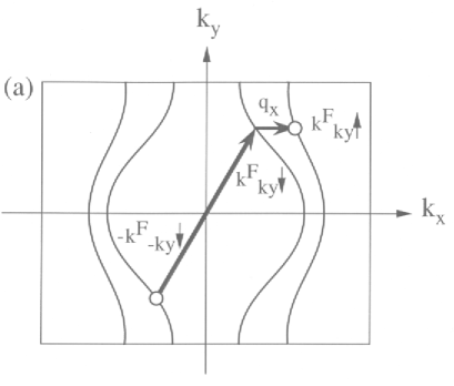
Fig.  1: (a) Schematic Q1D Fermi surface in $k_{x}$-$k_{y}$ plane in a magnetic field. (b) $a(k^{\rm F}_{k_{y},\sigma}-k^{\rm F}_{k_{y},\bar{\sigma}})$ as a function of $k_{y}/(b\pi)$. We take parameters as $t_{b}/t_{a}=0.1$, $t_{4b}/t_{b}=0$, quarter filled band and $H=5$Tesla. The long-dashed (dotted) line represents the $x$-component $aq_{x}(s)=2sa\mu_{\rm B}H/v_{\rm F}$ of the “nesting” vector a$q$ in $s=1.0(0.9)$.

In Fig. 2, we plot $T_{\rm c}(H)$ of the isotropic superconductivity obtained from eq. (9). In the following, we take parameters as $2t_{a}=1950$K, $t_{b}/t_{a}=0.1$, $t_{4b}/t_{b}=0$, $T_{\rm c}(0)=1.35$K. The maximum value of $T_{\rm c}(H)$ for each $H$ is obtained by optimizing $q_{x}(s)$.

The lines with squares, solid circles and open circles in Fig. 2 are obtained for $t_{c}/t_{a}=0$, which corresponds to no orbital effect. The optimized $T_{\rm c}(H)$ in the absence of higher harmonic terms is plotted by the line with solid circles. We find that the critical field at $T=0$, $H^{\rm LOFF}_{\rm P}\sim 6.0$T is more than two times larger than the Pauli paramagnetic limit $H_{\rm P}=1.84T_{\rm c}(0)\cong 2.5$T. This result is also larger than that of the squares, where the nesting vector $q$ is fixed to be $2\mu_{\rm B}H/v_{\rm F},(s=1)$ as studied by Lebed ${}^{\hbox{\immediate{?})}}$ ($H^{\rm LOFF}_{\rm P}\cong 0.6\sqrt{t_{a}/t_{b}}H_{\rm P}\sim 4.7$T). By adding the higher harmonic terms $t_{2b}/t_{b}=-0.1$ and $t_{3b}/t_{b}=-0.07$, $H^{\rm LOFF}_{\rm P}$ becomes larger (the open circle line in Fig. 2, $H^{\rm LOFF}_{\rm P}\sim 9$T). The enhancement of $T_{c}(H)$ and $H^{\rm LOFF}_{\rm P}$ due to the optimization of $q$ and the higher harmonic terms ($t_{2b}<0$) can be understood by the “nesting” of the Fermi surface as follows. At low temperatures, only electrons with $v^{\rm F}_{k_{y},\sigma}|k^{\rm F}_{k_{y},\sigma}-k^{\rm F}_{k_{y},\bar{\sigma}}+\alpha q_{x}|<\delta\sim T$ can contribute to forming Cooper pairs. The area on the Fermi surface, where $v^{\rm F}_{k_{y},\sigma}|k^{\rm F}_{k_{y},\sigma}-k^{\rm F}_{k_{y},\bar{\sigma}}+\alpha q_{x}|<\delta$, is proportional to $\sqrt{\delta}$ as $\delta\rightarrow 0$ if down Fermi surface touches the up Fermi surface by the translation of $q$, while it is proportional to $\delta$ if two Fermi surfaces cross by the translation. Since $\sqrt{\delta}\gg\delta$ for $\delta\rightarrow 0$, $H^{\rm LOFF}_{\rm P}$ becomes largest when the Fermi surfaces touch by the translation, which is equivalent to the case when $q_{x}(s)$ touches $k^{\rm F}_{k_{y},\sigma}-k^{\rm F}_{k_{y},\bar{\sigma}}$ in Fig. 1(b). The enhancement of $H^{\rm LOFF}_{\rm P}$ in 2D by this mechanism has been studied by Shimahara. ${}^{\hbox{\immediate{\bf{?}})}}$ These are two possibilities of choosing optimal $q_{x}(s)$, i.e., $q_{x}(s)$ touches $k^{\rm F}_{k_{y},\sigma}-k^{\rm F}_{k_{y},\bar{\sigma}}$ at $k_{y}\approx 0$ or $k_{y}\approx\pm\pi/b$. It may depend on the curvature of the Fermi surface and the Fermi velocity that which $q_{x}(s)$ gives the higher $H^{\rm LOFF}_{\rm P}$. We found that $H^{\rm LOFF}_{\rm P}$ is the largest when $q_{x}(s)$ touches at $k_{y}\approx 0$. If we take the positive $t_{2b}$, the “nesting” becomes worse at $k_{y}\approx 0$, although it becomes better at $k_{y}\approx\pm\pi/b$ as shown by the dot-dashed line Fig. 1(b). In this case $H^{\rm LOFF}_{\rm P}$ is not enhanced. We get $H^{\rm LOFF}_{\rm P}\approx 5.8$T for $t_{2b}/t_{b}=0.1$ and $t_{3b}/t_{b}=-0.07$. On the other hand $k^{\rm F}_{k_{y},\sigma}-k^{\rm F}_{k_{y},\bar{\sigma}}$ becomes flatter at $k_{y}\approx 0$ when $t_{2b}$ is negative as shown by the dashed line in Fig. 1(b), resulting in the better “nesting” and larger $H^{\rm LOFF}_{\rm P}$, as shown by the line with open circles in Fig. 2.

Next, we take the effect of orbital motions into account. Since the field dependence of the initial slope ${\rm d}H^{b}_{\rm c2}/{\rm d}T|_{T_{\rm c}(0)}$ is approximately given by the parameter $t_{c}t_{a}$ ${}^{\hbox{\immediate{?},\penalty 1000\hskip 0.91003pt plus 0.70004pt minus 0.70004pt{?})}}$ in the week field limit, we take parameters as $2t_{a}\sim 1950$K, $2t_{c}\sim 3.0$K, $a\sim 7\AA$, $c\sim 13\AA$ and $T_{\rm c}(0)\sim 1.35$K in order to fit the initial slope observed in (TMTSF)₂ClO₄ .${}^{\hbox{\immediate{?},\penalty 1000\hskip 0.91003pt plus 0.70004pt minus 0.70004pt{?})}}$ The transition temperature is plotted as the thick solid line in Fig. 2. This curve seems to be consistent with the experiments in organic superconductors (TMTSF)₂X by Lee et al .${}^{\hbox{\immediate{?},\penalty 1000\hskip 0.91003pt plus 0.70004pt minus 0.70004pt{?})}}$

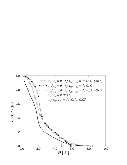
Fig.  2: Transition temperature $T_{\rm c}(H)$ of an isotropic pairing as a function of the magnetic field in the case of $t_{b}/t_{a}=0.1$, $t_{4b}/t_{b}=0$, $T_{\rm c}(0)=1.35$K for quarter filled electrons. The lines with squares and open circles and thick solid line are obtained from the optimal $q_{x}(s)$ giving the maximum value of $T_{\rm c}(H)$. If $s$ is fixed in $1.0$, we get the line with solid circles.

We also study $T_{\rm c}(H)$ of an anisotropic spin-singlet state. As shown in our previous paper ,${}^{\hbox{\immediate{?})}}$ the linearized gap equation for the anisotropic spin-singlet state is given by

$$\Delta(x)=2UT\sum_{k_{y},k_{z}}\cos^{2}(ck_{z})\sum_{\alpha,\omega_{n}}\int_{|x-x^{\prime}|>d}{\rm d}x^{\prime}\Delta(x^{\prime})$$

$$\times G^{\alpha}_{\uparrow}(x,x^{\prime},k_{y},k_{z},\omega_{n})G^{\bar{\alpha}}_{\uparrow}(x,x^{\prime},-k_{y},-k_{z},-\omega_{n}).$$ (13)

where $U$ is the nearest-site attractive interaction along the $c$ axis. The energy gap is zero at the lines $|ck_{z}|=\pi/2$ in this model. As in the isotropic case, eq. (13) is written as a matrix equation

$$\Delta^{Q}_{2l}=2U\sum_{l^{\prime}}\sum_{N}\sum_{k_{y}}D^{N}_{l,l^{\prime}}(k_{y})\tilde{K}_{k_{y}}(Q+NG)\Delta^{Q}_{2l^{\prime}},$$ (14)

where $\tilde{K}_{k_{y}}(q_{x})$ is given in eq. (12) and the coefficients $D^{N}_{l,l^{\prime}}(k_{y})$ is defined by

$$D^{N}_{l,l^{\prime}}(k_{y})=\frac{1}{4}\left[M^{1}_{N,l,l^{\prime}}(k_{y})+M^{-1}_{N,l,l^{\prime}}(k_{y})+2M^{0}_{N,l,l^{\prime}}(k_{y})\right],$$ (15)

where $M^{j}_{N,l,l^{\prime}}(k_{y})$ is given by

$$M^{j}_{N,l,l^{\prime}}(k_{y}) = \sum_{n}J_{n+l}(\eta^{\alpha}_{k_{y},\sigma})J_{n+l^{\prime}+j}(\eta^{\alpha}_{k_{y},\sigma})$$ (16)

$$\times J_{n-l+N}(\eta^{\alpha}_{k_{y},\bar{\sigma}})J_{n-l^{\prime}+N-j}(\eta^{\alpha}_{k_{y},\bar{\sigma}}).$$

In Fig. 3, we plot $T_{\rm c}(H)$ of an anisotropic spin-singlet superconductivity. Since the initial slope of the anisotropic spin singlet state is $\sqrt{2}$ times larger than that in the isotropic state ,${}^{\hbox{\immediate{?})}}$ we take parameters as $2t_{a}\sim 2070$K and $2t_{c}\sim 4.0$K in order to fit the experimental results. Other parameters are same as in the isotropic pairing case.

Fig.  3: Transition temperature $T_{\rm c}(H)$ of the anisotropic pairing as a function of the magnetic field.

If $U=\lambda$ and $t_{c}=0$ ($\eta^{\alpha}_{k_{y},\sigma}=0$), $T_{\rm c}(H)$ of an anisotropic spin-singlet is same as an isotropic pairing since $S^{N}_{l,l^{\prime}}(k_{y})=D^{N}_{l,l^{\prime}}(k_{y})=\delta_{l0}\delta_{l^{\prime}0}\delta_{N0}$. When $t_{c}\neq 0$, the behavior of $T_{\rm c}(H)$ for an anisotropic spin-singlet state is different from that for the isotropic case, but the difference between them is small.

In conclusion, we have calculated $T_{\rm c}(H)$ of the isotropic and anisotropic spin-singlet superconductivity in Q1D electrons. Although the Zeeman splitting strongly suppresses the superconductivity, the critical magnetic field is enhanced by choosing the optimal “nesting vector” and taking account of the higher harmonic terms in the energy dispersion. This result seems to be consistent with $T_{\rm c}(H)$ observed in the (TMTSF)₂X ,${}^{\hbox{\immediate{?},\penalty 1000\hskip 0.91003pt plus 0.70004pt minus 0.70004pt{?},\penalty 1000\hskip 0.91003pt plus 0.70004pt minus 0.70004pt{?})}}$ which may show not only the possibility of spin-singlet pairing in this system but importance of higher harmonic terms.

References

References

[1] A. G. Lebed: JETP Lett. 44 (1986) 114.
[2] N. Dupuis, G. Montambaux and C. A. R. S de Melo: Phys. Rev. Lett. 70 (1993) 2613.
[3] N. Dupuis and G. Montambaux: Phys. Rev. B 49 (1994)
8993.
[4] Y. Hasegawa and M. Miyazaki: J. Phys. Soc. Jpn. 65
(1996) 1028.
[5] M. Miyazaki and Y. Hasegawa: J. Phys. Soc. Jpn. 65
(1996) 3238.
[6] M. Miyazaki, K. Kishigi and Y. Hasegawa: J. Phys. Soc.
Jpn. 67 (1997) 2618.
[7] C. A. R. S de Melo:The
Superconducting State in Magnetic Fields (World Scientific, Singapore,
1998)
[8] I. J. Lee et al.:
Appl. Superconductivity 2 (1994) 753.
[9] I. J. Lee et al.:
Synth. Met. 70 (1995) 747.
[10] I. J. Lee et al.: Phys. Rev. Lett. 78 (1997)
1481.
[11] A. A. Abrikosov: Zh. Eksp Teor. Fiz. 32 (1957)
1442.
[12] L. P. Gor’kov: Zh. Eksp. Teor. Fiz. 37 (1959) 833.
[13] A. M. Clogston: Phys. Rev. Lett. 9 (1962) 266.
[14] B. S. Chandrasekhar: Appl. Phys. Lett. 1 (1962) 7.
[15] P. Fulde and A. Ferrell: Phys. Rev. 135 (1964)
A550.
[16] A. I. Larkin and Yu. N. Ovchinnikov: Sov. Phys. JETP
20 (1965) 762.
[17] A. G. Lebed: Phys. Rev. B 59 (1999) R721.
[18] L. P. Gor’kov and A. G. Lebed: J. Phys. Lett. bf 45
(1984) L433.
[19] G. Montambaux, M. Heritier and P. Lederer: Phys. Rev.
Lett. 55 (1985) 2078.
[20] K. Yamaji: J. Phys. Soc. Jpn. 54 (1985) 1034.
[21] D. Zanchi and G. Montambaux: Phys. Lev. Lett. 77
(1996) 366.
[22] N. Dupuis and V. M. Yakovenko: Phys. Rev. B 58
(1998) 8773.
[23] M. Takigawa, H. Yasuoka and G. Saito:
J. Phys. Soc. Jpn. 56
(1987) 873.
[24] S. Belin and K. Behnia: Phys. Rev. Lett. 79 (1997)
2125.