Quantum kinetic theory VII: The influence of vapor dynamics on condensate growth

Abstract

We extend earlier models of the growth of a Bose-Einstein condensate [1, 2, 3] to include the full dynamical effects of the thermal cloud by numerically solving a modified quantum Boltzmann equation. We determine the regime in which the assumptions of the simple model of [3] are a reasonable approximation, and compare our new results with those that were earlier compared with experimental data. We find good agreement with our earlier modelling, except at higher condensate fractions, for which a significant speedup is found. We also investigate the effect of the final temperature on condensate growth, and find that this has a surprisingly small effect.

The particular discrepancy between theory and experiment found in our earlier model remains, since the speedup found in these computations does not occur in the parameter regime specified in the experiment.

I Introduction

The fundamental process in the growth of a Bose-Einstein condensate is that of bosonic stimulation, by which atoms are scattered into and out of the condensate at rates enhanced by a factor proportional to the number of atoms in the condensate. This was first quantitatively considered by Gardiner et al. [1], in a paper which treated the idealized case of the growth of a condensate from an nondepletable “bath” of atoms at a fixed positive chemical potential $\mu$ and temperature $T$. This gave rise to a simple and elegant formula known as the simple growth equation

$$\dot{n}_{0}=2W^{+}(n_{0})\left\{\left(1-\mbox{e}^{[\mu_{\rm C}(n_{0})-\mu]/kT}\right)n_{0}+1\right\},$$ (1)

in which $n_{0}$ is the population of the condensate, $\mu$ is the chemical potential of the thermal cloud, and $\mu_{\rm C}(n_{0})$ is the condensate eigenvalue. The prefactor $W^{+}(n_{0})$ is a rate with an expression derived from quantum kinetic theory [4], which was estimated approximately in [1] by using a classical Boltzmann distribution. To go beyond the Boltzmann approximation for $W^{+}$ involves a very much more detailed treatment of the populations of the trap levels with energy less than $\mu$, since the equilibrium Bose-Einstein distribution for $\mu>0$ is not consistent with energies less than $\mu$. In other words, the populations of the lower trap levels cannot be treated as time-independent, and thus the dynamics of growth must include at least this range of trap levels as well as the condensate level. Therefore in [2, 3] we considered a less simplified model, covering a range of energies up to a cut-off, $E_{R}$, above which the system was assumed to be a thermal cloud with a fixed temperature and chemical potential. Equations were derived for the rate of growth of these levels along with the condensate, and the rates at which particles from the thermal bath scattered these quasi-particles between levels within the condensate band. The results of calculations showed that a speedup of the growth rate by a factor of the order of 3–4 compared to the simple growth equation could be expected, and that the initial part of the growth curve would be modified, leading to a much sharper onset of the initiation of the condensate growth.

The only experiment that has been done on condensate growth [11] was then under way. In these experiments clouds of sodium atoms were cooled to just above the transition temperature, at which point the high energy tail of the distribution was rapidly removed by an very severe RF “cut”, where the frequency of the RF field was quickly ramped down. After a short period of equilibration, the resulting vapor distribution was found to be similar to the assumptions of our theoretical treatments, and condensate growth followed promptly. The results obtained were fitted to solutions of the simple growth equation (1). When experimental results became available a speedup of about the predicted factor was found, and indeed the higher temperature results agreed very well with the theoretical predictions. At lower temperatures there was still some disparity; the theory predicted a slower rate of growth with decreasing temperature, but experimentally the opposite was observed.

The situation in which we now find ourselves leaves no alternative other than to address the remaining approximations. In our previous work we have made four major approximations:

• The part of the vapor with energies higher than $E_{R}$ has been treated as being time independent.

• The energy levels above the condensate level were modified phenomenologically to account for the fact that they must always be greater than the condensate chemical potential, which rises as the condensate grows.

• We treated all levels as being particle-like, on the grounds that detailed calculations [12] have shown that only a very small proportion of excitations of a trapped Bose gas are not of this kind.

• We have used the quantum Boltzmann equation in a ergodic form, in which all levels of a similar energy are assumed to be equally occupied.

In this paper we will no longer require the first two of these approximations. Abandoning the first means that we are required to take care of all kinds of collisions which can occur, and thus treat the time-dependence of all levels. This comes at a dramatic increase in both the computation time required (hours rather than seconds) and the precision of algorithms required. We also use a density of states which should be close to the actual density of states as the condensate grows, thereby avoiding the phenomenological modification of energy levels. However, we still treat all of the levels as being particle-like, since it seems unlikely that the few non-particle-like excitations will have a significant effect on the growth as a whole. The ergodic form of the quantum Boltzmann is needed to make the computations tractable, and is of necessity retained.

II Formalism

The basis of our method is Quantum Kinetic theory, a full exposition of which is given in Ref. [4]. These develop a complete framework for the study of a trapped Bose gas in a set of master equations. The full solution of these equations is not feasible, however, and therefore some type of approximation must be made. The basic structure of the method used here is essentially the same as that of QKVI, the major difference being that all time-dependence of the distribution function is retained. As explained in [3, 10], quantum kinetic theory leads to a model which can be viewed as a modification of the quantum Boltzmann equation in which

• The condensate wavefunction and energy eigenvalue—the condensate chemical potential $\mu_{\rm C}(n_{0})$—are given by the solution of the time-independent Gross-Pitaevskii equation with $n_{0}$ atoms.

• The trap levels above the condensate level are the quasiparticle levels appropriate to the condensate wavefunction. This leads to a density of states for the trap levels which is substantially modified, as discussed below in Sect. III B

• The transfer of atoms between levels is given by a modified quantum Boltzmann equation (MQBE) in the energy representation. This makes the ergodic assumption; that the distribution function depends only on energy.

A The ergodic form of the quantum Boltzmann equation

The derivation of the ergodic form of the quantum Boltzmann equation used by [13] is particular to the undeformed harmonic potential, and we give here a derivation appropriate to our case, in which the density of states can change with time as the condensate grows. We bin the phase space into energy bands labeled by the index $n$ with energies in a range $D_{n}(t)\equiv\left(\varepsilon_{n}(t)-{\delta\varepsilon_{n}(t)\over 2},\varepsilon_{n}(t)+{\delta\varepsilon_{n}(t)\over 2}\right)$ of width $\delta\varepsilon_{n}(t)$, and these widths change in time so that the number of states within each bin, $g_{n}$ is constant in time.

Starting from the full quantum Boltzmann equation the ergodic approximation is expressed in terms of this binned description as follows: We set $f({\bf x},{\bf K},t)$ equal to a constant, $f_{n}$, when $\epsilon({\bf x},{\bf K},t)\equiv{\hbar^{2}{\bf K}^{2}/2m}+V_{\rm eff}({\bf x},t)$ is inside the $n$th bin, i.e., $\epsilon({\bf x},{\bf K},t)\in D_{n}(t)$. (Here $V_{\rm eff}({\bf x},t)$ is the potential of the trap, as modified by the mean field arising from the presence of the condensate, as explained in QKV and QKVI.)

Thus we can approximate

$${\partial f({\bf x},{\bf K},t)\over\partial t}\to{\partial f_{n}\over\partial t}\mbox{\qquad if\qquad}\epsilon({\bf x},{\bf K},t)\in D_{n}(t),$$ (2)

In order to derive the ergodic quantum Boltzmann equation, we define the indicator function $\chi_{n}({\bf x},{\bf K},t)$ of the $n$th bin $D_{n}(t)$ by

$$\chi_{n}({\bf x},{\bf K},t) = 1\mbox{\qquad if\qquad}\epsilon({\bf x},{\bf K},t)\in D_{n}(t),$$ (3)

$$= 0\mbox{\qquad otherwise.}$$ (4)

The number of states in the bin $n$ will be given by $g_{n}=\int d^{3}{\bf x}d^{3}{\bf K}\,\chi_{n}({\bf x},{\bf K},t)/h^{3}$, and is held fixed.

The formal statement of the binned approximation is

$$f({\bf x},{\bf K},t)\to\sum_{n}f_{n}\chi_{n}({\bf x},{\bf K},t),$$ (5)

and the ergodic quantum Boltzmann equation is derived by substituting (5) into the various parts of the quantum Boltzmann equation as follows. For the time derivative part we make this replacement, and project onto $D_{n}(t)$, getting

$$\int{d^{3}{\bf x}d^{3}{\bf K}\over h^{3}}\chi_{n}({\bf x},{\bf K},t){\partial f({\bf x},{\bf K},t)\over\partial t} \to g_{n}{\partial f_{n}\over\partial t}.$$ (6)

[Note that the expansion (5) would mean that delta function singularities at the upper and lower boundaries of $D_{n}(t)$ would arise by differentiating $f({\bf x},{\bf K},t)$ as defined in (5), but the condition that $g_{n}$ be fixed means that these are of equal and opposite weight, and cancel when integrated over $D_{n}(t)$, givng a result consistent with (6).] We now replace ${\partial f({\bf x},{\bf K},t)/\partial t}$ on the left hand side of (6) by the collison integral that appears on the right hand side of the quantum Boltzmann equation, and substitute for $f({\bf x},{\bf K},t)$ in the collision integral using (5). [The streaming terms give no contribution, since the form (5) is a function of the energy $\epsilon({\bf x},{\bf K},t)$.]

This leads to the ergodic quantum Boltzmann equation in the form

 

$$g_{n}{\partial f_{n}\over\partial t} = {4a^{2}h^{3}\over m^{2}}\sum_{pqr}\left\{f_{p}f_{q}(1+f_{r})(1+f_{n})-(1+f_{p})(1+f_{q})f_{r}f_{n}\right\}\int{d^{3}{\bf x}d^{3}{\bf K}\over h^{3}}\int{d^{3}{\bf K}_{1}}\int{d^{3}{\bf K}_{2}}\int{d^{3}{\bf K}_{3}}$$ (9)

$$\times\chi_{n}({\bf x},{\bf K}_{1},t)\chi_{p}({\bf x},{\bf K}_{2},t)\chi_{q}({\bf x},{\bf K}_{3},t)\chi_{r}({\bf x},{\bf K},t)\delta\left({\bf K}_{1}+{\bf K}_{2}-{\bf K}_{3}-{\bf K}\right)$$

$$\times\delta\left(\epsilon({\bf x},{\bf K}_{1},t)+\epsilon({\bf x},{\bf K}_{2},t)-\epsilon({\bf x},{\bf K}_{3},t)-\epsilon({\bf x},{\bf K},t)\right).$$

The final integral is now approximated by the method of[13] to give [$a$ and $\bar{\omega}$ are defined in Sect. III]

$$g_{n}{\partial f_{n}\over\partial t} = {8ma^{2}\bar{\omega}^{2}\over\pi\hbar}\sum_{pqr}\left\{f_{p}f_{q}(1+f_{r})(1+f_{n})-(1+f_{p})(1+f_{q})f_{r}f_{n}\right\}{M(p,q,r,n)}\Delta(p,q,r,n).$$ (10)

Here $\Delta(p,q,r,n)$ is a function which expresses the overall energy conservation, and is defined by

$$\Delta(p,q,r,n) = 1\mbox{ when }|\varepsilon_{p}+\varepsilon_{q}-\varepsilon_{r}-\varepsilon_{n}|\leq{\left|\delta\varepsilon_{p}+\delta\varepsilon_{q}+\delta\varepsilon_{r}+\delta\varepsilon_{n}\right|\over 2},$$ (11)

$$= 0\mbox{ otherwise}.$$ (12)

 

Because we approximate $f({\bf x},{\bf K},t)$ by a constant value within each $D_{n}(t)$, energy conservation means that $\bar{E}\equiv\sum_{n}\varepsilon_{n}g_{n}f_{n}(t)$ is constant. This follows from energy conservation in the full quantum Boltzmann equation, which also implies that

$$\sum_{rn}\Delta(p,q,r,n)M(p,q,r,n)(\varepsilon_{r}+\varepsilon_{n})$$ (13)

$$\qquad=(\varepsilon_{p}+\varepsilon_{q})\sum_{rn}\Delta(p,q,r,n)M(p,q,r,n)$$ (14)

This is the limit to which the binning procedure defines energy conservation.

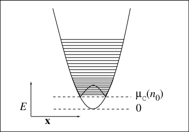
FIG. 1.: Qualitative picture of the compression of the quantum levels above the condensate mode as the condensate eigenvalue increases.

III Details of model

The most important aspect of our model is the inclusion of the mean field effects of the condensate. As the population of the condensate increases, the absolute energy of the condensate level also rises due to the atomic interactions. This results in a compression in energy space of the quantum levels immediately above the condensate, (see Fig. 1) and has an important effect on the evolution of the cloud.

The correct description of the quantum levels immediately above the ground state when there is a significant condensate population requires a quasiparticle transformation. This is computationally difficult, however, so we make use of a single-particle approximation for these states. This should be reasonable, as most of the growth dynamics will involve higher lying states that will be almost unaffected by the presence of the condensate. In [3] we did this using a linear interpolation of the density of states; here we use an approximate treatment based on the Thomas-Fermi approximation.

A Condensate chemical potential $\mu_{\rm C}(n_{0})$

We consider a harmonic trap with a geometric mean frequency of

$$\bar{\omega} = (\omega_{x}\omega_{y}\omega_{z})^{1/3}.$$ (15)

We include the mean field effects via a Thomas-Fermi approximation for the condensate eigenvalue, which is directly related to the number of atoms in the condensate mode. As in [3, 10], we use a modified form of this relation in order to give a smooth transition to the correct harmonic oscillator value when the condensate number is small:

$$\mu_{\rm C}(n_{0})=\alpha\left[n_{0}+({3\hbar\bar{\omega}}/{2\alpha})^{5/2}\right]^{2/5},$$ (16)

where $\alpha=(15a\bar{\omega}m^{1/2}\hbar^{2}/4\sqrt{2})^{2/5}$, and $a$ is the atomic s-wave scattering length. Thus, for $n_{0}=0$ we have $\mu_{\rm C}(0)=\varepsilon_{0}=3\hbar\bar{\omega}/2$.

B Density of states $\bar{g}(\varepsilon)$

We assume a single particle energy spectrum with a Bogoliubov-like dispersion relation, as in Timmermans et al. [14], which leads to a density of states of the form

 

$$\bar{g}(\varepsilon,n_{0}) = \frac{4}{\pi}\frac{\mu_{\rm C}(n_{0})^{2}}{(\hbar\bar{\omega})^{3}}\left[\left(\frac{\varepsilon}{\mu_{\rm C}(n_{0})}-1\right)\int_{0}^{1}dx\sqrt{1-x}\frac{\left[\sqrt{(\varepsilon/\mu_{\rm C}(n_{0})-1)^{2}+x^{2}}-x\right]^{1/2}}{\sqrt{(\varepsilon/\mu_{\rm C}(n_{0})-1)^{2}+x^{2}}}+\int_{1}^{\varepsilon/\mu_{\rm C}(n_{0})}dx\sqrt{x}\sqrt{{\varepsilon\over\mu_{\rm C}(n_{0})}-x}\right],$$ (17)

This integral can be carried out analytically; the result is

$$\bar{g}(\varepsilon,n_{0}) = \frac{\varepsilon^{2}}{2(\hbar\bar{\omega})^{3}}\left\{1+q_{1}\left(\mu_{\rm C}(n_{0})/\varepsilon\right)+\left(1-\frac{\mu_{\rm C}(n_{0})}{\varepsilon}\right)^{2}q_{2}\left(\frac{1}{\varepsilon/\mu_{\rm C}(n_{0})-1}\right)\right\},$$ (19)

where

$$q_{1}(x) = \frac{2}{\pi}\left[\sqrt{x}\sqrt{1-x}(1-2x)-\sin^{-1}(\sqrt{x})\right],$$ (20)

$$q_{2}(x) = \frac{4\sqrt{2}}{\pi}\left[\sqrt{2x}+x\log\left(\frac{1+x+\sqrt{2x}}{\sqrt{1+x^{2}}}\right)-\left\{\frac{\pi}{2}+\sin^{-1}\left(\frac{x-1}{\sqrt{1+x^{2}}}\right)\right\}\right].$$ (21)

 

This is plotted in Fig. 2, along with that for the ideal gas. Thus the density of states of the trap varies smoothly as the condensate grows.

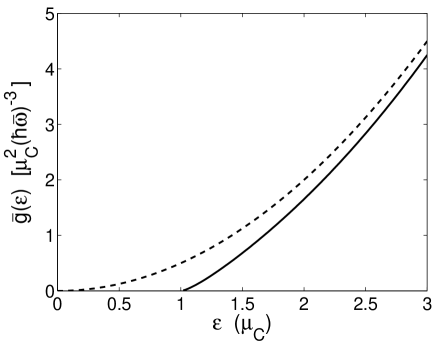
FIG. 2.: The modified density of states (solid curve) compared with non-interacting function (dashed curve) for the harmonic trap.

IV Numerical methods

A Representation

The bins we shall choose for the representation of the distribution in terms of the quantities $f_{n}$ as in (5) are divided into two distinct regions, as shown diagrammatically in Fig. 3. The lowest energy region corresponds essentially to the condensate band $R_{C}$ of [1, 3, 7, 10]. This is the region in which $f_{n}$ is rapidly varying in the regime of quantum degeneracy, and is described by a series of fine-grained energy bins up to an energy $E_{R}\approx 3\mu_{\rm C}(n_{0,{\rm max}})$. The condensate is a single quantum state represented by the lowest energy bin.

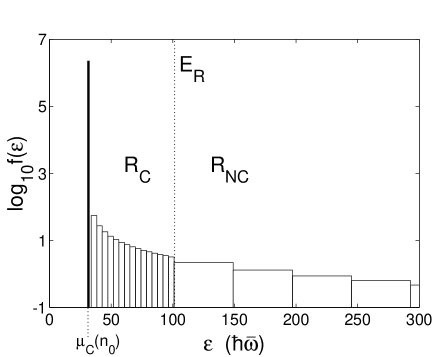
FIG. 3.: The numerical representation of the system with a condensate of $2.3\times 10^{6}$ atoms at a temperature of $590$nK. $R_{C}$ is the condensate band, which is fine-grained, whereas $R_{NC}$ is the non-condensate band, which is coarse-grained. The division between the two bands is fixed at $E_{R}$. The condensate energy is derived from the Thomas-Fermi approximation.

As the number of particles in the condensate changes, the energy of the condensate level changes according to the Thomas-Fermi approximation of Eq. 16. Thus the total energy width of $R_{C}$ decreases as the condensate grows.

We represent $R_{C}$ by a fixed number of energy bins of equal width $\delta\varepsilon_{n}$ with a midpoint of $\varepsilon_{n}$ .

As the condensate energy increases, we adjust $\varepsilon_{n}$ and $\delta\varepsilon_{n}$ between integration timesteps, such that the widths of the bins remain equal. This is done by redistributing the numbers of particles into new bins after each timestep, and thus does not contradict the requirement that $g_{n}$ is fixed during the timestep. We find that this is the most simple procedure for the calculation of rates in and out of these levels. We choose the number of bins to be sufficient such that the width is not more than about $\delta\varepsilon_{n}\sim 5\hbar\bar{\omega}$.

The high energy region corresponds to the thermal bath of our previous papers. This is the region in which $f_{n}$ is slowly varying, and therefore the energy bins are considerably broader (up to $64\hbar\bar{\omega}$ in the results presented in this paper). The evaporative cooling is carried out by the sudden removal of population of the bins in this region with $\varepsilon_{n}>\varepsilon_{\rm cut}$.

B Solution

There are four different types of collision that can occur given our numerical description of the system. These are depicted in Fig. 4.

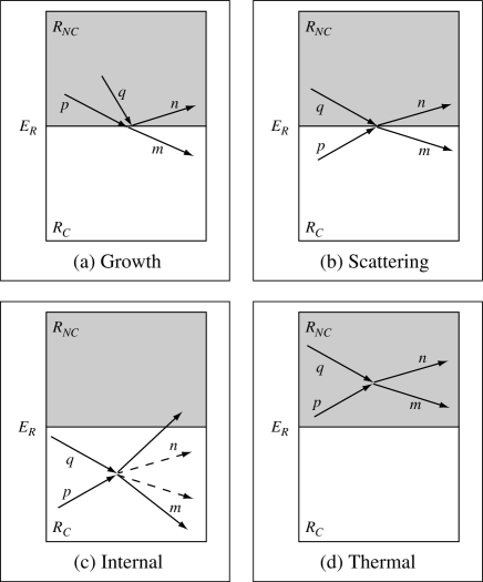
FIG. 4.: The four different collision types that can occur in our numerical description.

• Growth: This involves two particles in $R_{NC}$ colliding, resulting in the transfer of one of the particles to the condensate band (along with the reverse process).

• Scattering: A particle in $R_{NC}$ collides with a particle in the condensate band, with one particle remaining in $R_{C}$.

• Internal: Two particles within the condensate band collide with at least one of these particles remaining in $R_{NC}$ after the collision.

• Thermal: This involves all particles involved in the collision coming from the non-condensate band and remaining there.

Our first description of condensate growth [1] considered only process (a). The next calculation [2, 3] involved both process (a) and (b). The calculations presented below include all four processes, allowing us to determine whether the earlier approximations were justified.

The computation of the rates of processes (a) and (b) is made difficult because of the different energy scales of the two regions of the distribution function. Our solution is to interpolate the distribution function $f_{n}$ in $R_{NC}$ (non-condensate band) such that the bin sizes are reduced to be the same as for $R_{C}$ (the condensate band). The rates are then calculated using this interpolated distribution function, now consisting of more than one thousand bins, and the rates for the large bins of the non-condensate band are found by summing the rates of the appropriate interpolated bins.

We have found that these rates are extremely sensitive to the accuracy of the numerical interpolation — small errors lead to inconsistencies in the solutions of the MQBE. This procedure is more efficient than simply using the same bin size for the whole distribution, as there are only a small number of bins for the condensate band.

C Algorithm

The algorithm we use to solve the MQBE is summarised as follows

• Calculate the collision summation for all types of collisions, keeping the density of states, and the energies of the levels in the condensate band $R_{C}$ fixed. The distribution function $f_{n}(t+\delta t)$ is calculated using an embedded 4th order Runge-Kutta method, using Cash-Karp parameters [15].

• The quantity ${M(p,q,r,n)}$ defined by (10) expresses all the overlap integrals, and is quite difficult to compute exactly. In our computations we have simply set this to correspond to the value found in [13], i.e., we set

  $$M(p,q,r,n) = g_{{\rm min}(p,q,r,n)},$$ (22)

  and express energy conservation in a simplified form, using the fact that the energy bins will be chosen equally spaced, by choosing a Kronecker delta form

  $$\Delta(p,q,r,n) \to \delta(p+q,r+n).$$ (23)

  The difference between these two forms clearly goes to zero as the bins become very narrow.

  It has been explicitly checked that in practice energy is conserved to a very high degree of accuracy throughout the calculation.

• As a result of the time step, the condensate population will have changed. This causes the density of states to alter slightly, along with the positions and widths of the energy bins in the condensate band, as all these quantities are determined by the condensate number $n_{0}$. The derivation in Sect. II A shows that the populations $g_{n}f_{n}$ are of the bins which move with the change of energy levels and density of states as the condensate grows so as to maintain the number of levels $g_{n}$ in the bin constant. Therefore after the Runge-Kutta timestep, the numbers $g_{n}f_{n}$ represent the numbers of particles in the bins determined by the appropriate energy levels after that step.

• As a result of the preceding step, the bins will no longer of equal width, so we rebin the numbers of atoms into a new set of equally spaced bins, as explained Sect. IV A.

  To ensure total number conservation of particles, we keep the number of particles in each bin, $g_{n}f_{n}$ constant when we adjust the energies and widths of the bins. As the change in the density of states and the width of each bin is determined by the condensate number, the occupation per energy level of the $n$th bin, $f_{n}$, must be altered slightly to ensure number conservation.

• We now continue with step (1).

The change in $\mu_{C}(n_{0})$ with each time step, and hence the shifts in the energy of the bins in $R_{C}$ is very small. Hence, the adjustment of the distribution function due to step (3) is tiny, much smaller than the change due to step (1).

The method has been tested by altering the position of $E_{R}$ and width of the energy bins of $R_{NC}$ and $R_{C}$. We have found that the solution is independent of the value of $E_{R}$ over a large range of values of these parameters.

V Results

In this paper we present the results of simulations modelling the experiments described in [11]. In these experiments a cloud of sodium atoms confined in a ‘cigar’ shaped magnetic trap was evaporatively cooled to just above the Bose-Einstein transition temperature. Then, in a period of 10ms the high energy tail of the distribution was removed with a very rapid and rather severe RF cut. The condensate was then manifested by the formation of a sharp peak in the density distribution.

We have carried out a full investigation of the effect of varying the initial cloud parameters has on the growth of the condensate for the trap configuration described in [11]. In this paper we concentrate on a comparison of these results with our earlier theoretical model. To model these experiments, we begin our simulations with an equilibrium Bose-Einstein distribution, with temperature $T_{i}$ and chemical potential $\mu_{\rm init}$ and truncate it at an energy $\varepsilon_{\rm cut}=\eta kT_{i}$, which represents the system at the end of the RF sweep. This is then allowed to evolve in time, until the gas once again approaches an equilibrium the appropriate equilibrium Bose-Einstein in the presence of a condensate. This is pictured schematically in Fig. 5.

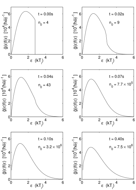
FIG. 5.: Snapshots of the distribution function for a simulation with initial conditions $\mu_{\rm init}=-100\hbar\bar{\omega}$, $T_{i}=1119$nK, and $\eta=2.83$. This results in a condensate with $n_{0}=7.5\times 10^{6}$ atoms at a temperature of $T_{f}=830$nK. For clarity, the condensate itself is not depicted, but the presence of a significant amount of condensate has the effect of displacing the left hand ends of the curves (d)–(f) an amount $\mu_{\rm C}(n_{0})/kT_{i}$ from the axis. The growth curve for this simulation is shown in Fig. 6(a).

Because of the ergodic assumption, the MQBE that we simulate depends only on the geometric average of the trapping frequencies $\bar{\omega}=(\omega_{x}\omega_{y}\omega_{z})^{1/3}$. There is likely to be some type of experimental dependence on the actual trap geometry which is not included in our simulation; however in the regime $kT\gg\hbar\bar{\omega}$ this should be small. The trap parameters of [11] were $(\omega_{x},\omega_{y},\omega_{z})=2\pi\times(82.3,82.3,18)$Hz , giving $\bar{\omega}=2\pi\times 49.6$Hz.

A Matching the experimental data

The main source of quantitative experimental data of condensate growth generally available is Fig. 5 of [11]. This gives growth rates as a function of final condensate number and temperature rather than the initial conditions. Whereas the growth curves calculated in [1, 3] required these parameters as inputs, the calculations presented here require three different input parameters; the initial number of atoms in the system $N_{i}$ (and hence the initial chemical potential $\mu_{\rm init}$), the initial temperature $T_{i}$, and the position of the cut energy $\eta kT_{i}$.

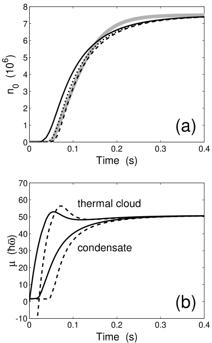
FIG. 6.: Growth of a condensate with $n_{0}=7.5\times 10^{6}$, $T_{f}=830$nK. Solid lines $\mu_{\rm init}=0$, dotted lines $\mu_{\rm init}=-40\hbar\bar{\omega}$, dashed lines $\mu_{\rm init}=-100\hbar\bar{\omega}.$ (a) Population of condensate versus time. Grey curve is the solution for model of [3]. (b) Chemical potential $\mu_{\rm C}(n_{0})$ of condensate (lower curves) and effective chemical potential $\mu_{\rm eff}$ of thermal cloud (upper curves).

Given the final parameters supplied in [11], it is possible to calculate a set of initial conditions that we require. As we know the final condensate number, we can calculate the value of the chemical potential of the gas using the Thomas-Fermi approximation for the condensate eigenvalue, Eq. 16. This gives a density of states according to Eq. 19, and along with the measured final temperature $T_{f}$, we can calculate the total energy $E_{\rm tot}$ and number of atoms $N_{\rm tot}$ in the system at the end of the experiment, completely characterizing the final state of the gas.

$$N_{\rm tot} = n_{0}+\sum_{\varepsilon_{n}>\mu_{\rm C}(n_{0})}^{\infty}\frac{g_{n}}{\exp[(\varepsilon_{n}-\mu_{\rm C}(n_{0}))/kT_{f}]-1},$$ (24)

$$E_{\rm tot} = E_{0}(n_{0})+\sum_{\varepsilon_{n}>\mu_{\rm C}(n_{0})}^{\infty}\frac{\varepsilon_{n}g_{n}}{\exp[(\varepsilon_{n}-\mu_{\rm C}(n_{0}))/kT_{f}]-1}.$$ (25)

We now want to find an initial distribution that would have the same total energy and number of atoms if truncated at $\varepsilon_{cut}=\eta kT_{i}$. If we specify an initial chemical potential for the distribution $\mu_{\rm init}$, we can self-consistently solve for the parameters $T_{i}$ and $\eta$ from the following non-linear set of equations

$$N_{\rm tot} = \sum_{\varepsilon_{n}=3\hbar\bar{\omega}/2}^{\eta kT_{i}}\frac{g_{n}}{\exp[(\varepsilon_{n}-\mu_{\rm init})/kT_{i}]-1},$$ (27)

$$E_{\rm tot} = \sum_{\varepsilon_{n}=3\hbar\bar{\omega}/2}^{\eta kT_{i}}\frac{\varepsilon_{n}g_{n}}{\exp[(\varepsilon_{n}-\mu_{\rm init})/kT_{i}]-1}.$$ (28)

This gives the input parameters for our simulation, and we can now calculate growth curves starting with initially different clouds, but resulting in the same final condensate number and temperature.

B Typical results

A sample set of growth curves is presented in Fig. 6(a), for a condensate with $7.5\times 10^{6}$ atoms at a final temperature of $830$nK and a condensate fraction of 10.4%. The initial parameters for the curves are given in Table I.

As can be seen the curves are very similar, and arguably would be difficult to distinguish in experiment. The main difference is the further the system starts from the transition point (i.e. the more negative the initial chemical potential), the longer the initiation time but the steeper the growth curve. This trend continues as $\mu_{\rm init}$ becomes more negative.

$\mu_{\rm init}(\hbar\bar{\omega})$	$T_{i}({\rm nK})$	$N_{i}(10^{6})$	$\eta$	$\varepsilon_{\rm cut}(\hbar\bar{\omega})$
0	1000	89.1	3.82	1605
-40	1080	100.1	3.31	1503
-100	1119	117.6	2.83	1419

TABLE I.: Parameters for the formation of a condensate with $n_{0}=7.5\times 10^{6}$ atoms at a temperature of $T_{f}=830{\rm nK}$ from an uncondensed thermal cloud. The growth curves are plotted in Fig. 6.

1 Effective chemical potential

To facilitate understanding of these results, we introduce the concept of an effective chemical potential $\mu_{\rm eff}$ for the non-condensate band. We do this by fitting a Bose-Einstein distribution to the lowest energy bins of $R_{NC}$ as a function of time. Obviously, the chemical potential is undefined when the system is not in equilibrium, but as has been noted for the classical Boltzmann equation [16], the distribution function tends to resemble an equilibrium distribution as evaporative cooling proceeds. The effective chemical potential is not unique—it is dependent on the particular choice of the energy cutoff $E_{R}$. It gives a good indication of the “state” of the non-condensate, however, since the majority of the particles entering the condensate after a collision come from these bins. In this paper $\mu_{\rm eff}$ was computed by a linear fit to $\log[1+1/f_{n}]$ of the first ten bins of the noncondensate band, with the intercept giving $\mu_{\rm eff}$ and the gradient the temperature.

2 Interpretation

We find that all the results presented in this paper can be qualitatively understood in terms of the simple growth equation Eq. (1), with the vapour chemical potential $\mu$ replaced by the effective chemical potential $\mu_{\rm eff}$ of the thermal cloud.

The simple growth equation requires $\mu_{\rm eff}>\mu_{\rm C}(n_{0})$ for condensate growth to occur. In Fig. 6(b) we plot the effective chemical potential $\mu_{\rm eff}$ of the thermal cloud and the chemical potential of condensate $\mu_{\rm C}(n_{0})$. This graphs helps explain the two effects noted above—longer initiation time and a steeper growth curve for the $\mu_{\rm init}=-100\hbar\bar{\omega}$ case. Firstly, the inversion of the chemical potentials for this simulation occurs at a later time than for $\mu_{\rm init}=0$, causing the stimulated growth to begin later. This is because the initial cloud for the $\mu_{\rm init}=-100\hbar\bar{\omega}$ simulation is further from the transition point at $t=0$. Secondly, the effective chemical potential of the thermal cloud rises more steeply, meaning that $\mu_{\rm eff}-\mu_{\rm C}(n_{0})$ is larger, and therefore the rate of condensate growth is increased.

C Comparison with earlier model

In Fig. 6(a) we have also plotted the growth curve that is calculated for these final condensate parameters by the model of [3], which we refer to as the simple model (not to be mistaken with the solution of the simple growth equation 1). For this earlier model the initial condensate number is indeterminate, whereas for the detailed calculation presented here the initial distribution is Bose-Einstein, with the zero of the time axis being the removal of the high energy tail.

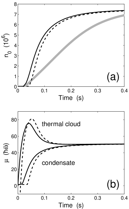
FIG. 7.: Comparison of condensate growth models for a condensate fraction of 24.1%, $n_{0}=7.5\times 10^{6}$, $T_{f}=590$nK. Solid lines $\mu_{\rm init}=0$, dashed lines $\mu_{\rm init}=-100\hbar\bar{\omega}.$ (a) Population of condensate versus time. Grey line is the solution for model of [3]. (b) Chemical potential of condensate (lower curves) and effective chemical potential of thermal cloud (upper curves).

For these particular parameters, it turns out that the results of the full calculation of the growth curve give very similar results to the previous model, with the initial condensate number adjusted appropriately. This is not surprising; indeed, from Fig. 6(b) we can see that the approximation of the thermal cloud by a constant chemical potential (i.e. the cloud is not depleted) is good for the region where the condensate becomes macroscopic.

For larger condensate fractions, however, the principal condition assumed in the model of [3], that the chemical potential of the vapor can be treated as approximately constant, is no longer satisfied. In Fig. 7(a) we plot the growth of the same size condensate as in Fig. 6, (that is, $7.5\times 10^{6}$ atoms) but at a lower final temperature of 590nK. In this situation the condensate fraction increases to 24.1%, and so there is considerable depletion of the thermal cloud. The effect of this can be seen in Fig. 7(b). The difference between the vapor and condensate chemical potentials $\mu_{\rm eff}-\mu_{\rm C}(n_{0})$ initially increases to much larger values than for the simple model, where $\mu_{\rm eff}$ is held constant at its final equilibrium value. It is this fact that causes more rapid growth.

As the condensate continues to grow, it begins to significantly deplete the thermal cloud, causing $\mu_{\rm eff}$ to decrease from its maximum. It is the “overshoot” of $\mu_{\rm eff}$ from the final equilibrium value that the model of [3] and QKVI cannot take account of. This overshoot only occurs for final condensate fractions of more than about ten percent; hence up to this value the simple model should be sufficient.

D Effect of the final temperature on condensate growth

We have investigated the effect that final temperature has on the growth of a condensate of a fixed number. All simulations were begun with $\mu_{\rm init}=0$, since the initial chemical potential has little effect on the overall shape of the growth curves. This determines the other parameters, $T_{i}$ and $\eta$ and the initial conditions are shown in Table II. The results of these simulations are presented in Fig. 8.

We find the somewhat surprising result that the growth curves do not change significantly over a very large temperature range for the same size condensate. In fact, a condensate formed at 600nK grows more slowly than at 400nK for these parameters. As the temperature is increased further, however, the growth rate increases again, and at a final temperature of 1$\mu$K the growth rate is faster than at 400nK. This effect has also been observed for both larger ($7.5\times 10^{6}$) and smaller ($1\times 10^{6}$) condensates.

This observation can once again be interpreted using the simple growth equation (1). Although $W^{+}(n_{0})$ increases with temperature (approximately as $T^{2}$ as shown in [1]), the maximum value of $\mu_{\rm eff}-\mu_{\rm C}(n_{0})$ achieved via evaporative cooling decreases with temperature for a fixed condensate number, as the cut required is less severe and the final condensate fraction is smaller. Also, the term in the curly brackets of Eq. 1 is approximately proportional to $T^{-1}$ for most regimes. The end result is that the decrease in this term compensates for the increase in $W^{+}(n_{0})$, giving growth curves that are very similar for the different simulations. Once the “overshoot” of the thermal cloud chemical potential ceases to occur (when the evaporative cooling cut is not as severe), the growth rate begins to increase with temperature as predicted by the model of [3] and QKVI.

FIG. 8.: Growth of a condensate with a final condensate size of $2.5\times 10^{6}$ atoms from a vapor with $\mu_{\rm init}=0$. The dotted line is for a final temperature of 400nK, dashed 600nK, and solid 1$\mu$K. (a) Growth curves. (b) Chemical potential of condensate (lower curves) and thermal cloud (upper curves).

$T_{f}({\rm nK})$	$T_{i}({\rm nK})$	$N_{i}(10^{6})$	$\eta$	$\varepsilon_{\rm cut}(\hbar\bar{\omega})$	Condensate fraction
400	622.0	21.5	2.19	572	0.253
600	707.3	31.6	4.03	1198	0.099
1000	1064.8	107.7	5.87	2629	0.025

TABLE II.: Parameters for the formation of condensate with $n_{0}=2.5\times 10^{6}$ atoms from an uncondensed thermal cloud with $\mu_{\rm init}=0$. The growth curves are presented in Fig. 8.

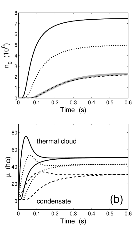
FIG. 9.: Growth of a condensate with at a final temperature of 590nK, starting from an uncondensed thermal cloud with $\mu_{\rm init}=0$. Solid line $7.5\times 10^{6}$ atoms, dotted line $5.0\times 10^{6}$ atoms, dashed $2.3\times 10^{6}$ atoms. The dashed line is for the same parameters as the lower temperature curves in [3]. (a) Growth curves, with the solution to the model of [3] in grey. (b) Chemical potential of condensate (lower curves) and thermal cloud (upper curves).

$n_{0}(10^{6})$	$T_{i}({\rm nK})$	$N_{i}(10^{6})$	$\eta$	$\varepsilon_{\rm cut}(\hbar\bar{\omega})$	Condensate fraction
2.3	692.5	29.6	4.07	1186	0.095
5.0	794.6	44.7	2.91	973	0.179
7.5	897.9	64.6	2.29	865	0.239

TABLE III.: Parameters for the formation of condensates at $T_{f}$ = 590nK from an uncondensed thermal cloud with $\mu_{\rm init}=0$. The growth curves are presented in Fig. 9

.

E Effect of size on condensate growth

Finally we have performed some simulations of the formation of a condensate at a fixed final temperature, but of a varying size. The parameters for these simulations are given in Table III, and the growth curves are plotted in Fig. 9(a). We find that the larger the condensate, the more rapidly it grows. The initial clouds required to form the larger condensates not only start at a higher temperature (and thus have a higher collision rate to begin with), but also they need to be truncated more severely, causing a larger difference in the chemical potentials, as seen in Fig. 9(b). Thus instead of these effects negating each other as in the previous section, here they tend to reinforce one another. This causes the growth rate to be highly sensitive to the final number of atoms in the condensate for a fixed final temperature.

For further comparison with the previous model, in Fig. 9(a) the dashed curve is for the same parameters as for the lower temperature results of [3], whose prediction is plotted in grey—as can be seen, the two methods are in very good agreement with each other for this choice of parameters. It is this particular set of final parameters for which the discrepancy between theory and experiment remains.

F The appropriate choice of parameters

In our computations we have taken some care to make sure that we can give our results as a function of the experimentally measured final temperature $T_{f}$ and condensate number $n_{0}$. Nevertheless, it can be seen from our results that this can give rise to counterintuitive behavior, such as the fact that under the condition of a given final condensate number, the growth rate seems to be largely independent of temperature, because of the cancellation noted in Sect. V D. This effect has its origin in the quite simple fact that with a sufficiently severe cut it is impossible to separate the process of equilibration of the vapor distribution to a quasiequilibrium from the actual process of growth of the condensate. In other words, the attempt to implement the “ideal” experiment in which a condensate grows from a vapor with a constant chemical potential and temperature cannot succeed with a sufficiently large cut. Under these conditions, the initial temperature differs quite strongly from the final temperature, and as well, the number of atoms required to produce the condensate is so large that the vapor cannot be characterized by a slowly varying chemical potential during most of the growth process.

G Comparison with experiment

1 Comparison with MIT fits

The most quantitative data available from [11] is in their Fig. 5, in which results are presented as parameters extracted from fits to the simple growth equation 1. In [3] we took two clusters of data from this figure, at the extremes of the temperature range for which measurements were made, and compared the theoretical results with the fitted experimental curves. At the higher temperature of 830nK the results were in good agreement with experiment, but at 590nK they differed significantly, the experimental growth rate being about three times faster than the theoretical result.

We have performed the same calculations using the detailed model. The results for 830nK are presented in Fig. 6 and those for 590nK are presented in Fig. 9. There is a good match between the two theoretical models at both temperatures.

2 Comparison with sample growth curves

In [11] some specific growth curves are also presented, and we shall compare these with with our computations, and those of Bijlsma et al. [17], which appeared in preprint form after the initial submission of this paper.

In Fig. 10 we show the data from Fig. 3 of [11], the computation of Fig. 11 of [17], and our own computations. This is for the MIT sodium trap, with the simulation parameters taken from Ref. [17] of $N_{i}=60\times 10^{6}$, $T_{i}=876$nK and $\eta=2.5$. We find this results in a condensate of $6.97\times 10^{6}$ atoms at a temperature of 604nK, and a final condensate fraction of 21.8% after half a second, which agrees with our predictions from the solution of the equations in Sect. V A at $t=\infty$ to within 0.2%.

We can see that there is little difference in the results of the two computations for this case, the main discrepancy being that the initiation time for our simulation is a little longer than that of Bijlsma et al. This is likely to be due to the fact that their calculation starts with the condensate already occupied with $n_{0}=5\times 10^{4}$ atoms, whereas we begin with the equilibrium number at this temperature given by the Bose distribution of $n_{0}=208$ atoms. This difference could be brought about by the use of a slightly different density of states, which is also the likely cause of the difference in the final condensate number, of approximately $3\times 10^{5}$ atoms.

The agreement with the experimental growth curve data is very good for both computations. The simpler model of [3] and QKVI cannot reproduce the results at this temperature, as is shown by the lower grey curve in Fig. 10. This is as we expect—the final condensate fraction is far greater than 10% and in this case the “overshoot” of $\mu_{\rm eff}$ is significant.

Given these initial conditions, this is the only case in which we have found that the “speedup” given by the full quantum Boltzmann theory may yield a significant improvement of the fit to the experimental data.

We would like to emphasise, however, that the parameters used for this simulation do not come from Ref. [11]. The MIT paper does not provide any details of the size of the thermal cloud, or the temperature at which this curve was measured, and as such, a set of unique initial and final parameters of the experiment cannot be determined. We have simply taken these parameters from the calculation of Ref. [17].

In fact, it seems likely to us that the final temperature for the experimental curve shown in Fig. 10 should be higher. Studying Fig. 5 of Ref. [11] shows that most condensates of $7\times 10^{6}$ atoms or more were formed at temperatures above 800nK. We have therefore performed a second calculation using the simple model with a final temperature of $830$nK, and this result is shown as the upper grey curve in Fig. 10. As can be seen, this also fits the experimental data extremely well. The condensate fraction at this higher temperature is 10.2%, meaning that these parameters are very similar to the situation considered in Fig. 6, which was originally found to be a good match to experimental data in Ref. [3]. We note that the solution to the simple model at this higher temperature is also in good agreement with our more detailed calculation for these parameters.

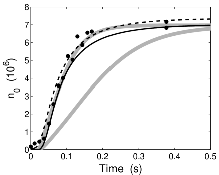
FIG. 10.: A comparision between the results of Fig. 11 of [17] and our own calculations with the initial conditions $N_{i}=60\times 10^{6}$ atoms, $T_{i}=876$nK, $\eta=2.5$. Our data is shown as the solid line and the results from Bijlsma et al. are the dashed line. The results of the simple model of condensate growth with a final temperature of $T_{f}=604$nK matching these initial conditions is lower grey curve. The upper grey curve is also for the simple model, but with what we feel is a more realistic final temperature of $T_{f}=830$nK. The experimental data points are the solid dots.

The situation is very different, however, if we compare with the result of Fig. 4 of [11], in which the final condensate number was $1.2\times 10^{6}$ atoms. In this case, the data of Fig. 4(b) of Ref. [11] can be used to extract all the relevant experimental parameters. This graph shows an experimentally measured reduction in the thermal cloud number from about $40\times 10^{6}$ atoms to about $15\times 10^{6}$ over the duration of the experiment. Including the final condensate population gives a total number of atoms in the system of approximately $16.2\times 10^{6}$, or a loss of about 60% of the atoms. With the three pieces of data taken from the MIT graphs (initial thermal cloud number, final thermal cloud number and final condensate number), we can estimate all the relevant parameters using the equations of Sect. V A, and these are shown in the second column of Table IV.

While the parameters we present here are consistent with the static experimental data, the growth curve corresponding to these parameters (shown in Fig. 11) certainly does not fit the dynamical data. We find that to remove such a large proportion of atoms, yet still obtain a relatively small condensate, the initial system must be a long way from the transition temperature, with $\mu_{\rm init}=-212\hbar\bar{\omega}$.

This means that condensate growth does not occur until the relaxation of the thermal cloud is almost complete, resulting in a very long initiation time, Also, when the growth does begin, the rate is significantly slower than was experimentally observed. This is the region in which the experimental and theoretical discrepancies lie.

Quantity	Parameters extracted from experiment	Parameters which give an apparent fit
$N_{i}$ ($10^{6}$)	40.0	40.0
Atoms lost	60%	94%
Condensate fraction	7.2%	51%
$T_{i}$ (nK)	945.5	765
$T_{f}$ (nK)	530	211
$\eta$	2.19	0.60

TABLE IV.: Comparison of the static parameters of the Bose gas that match Fig. 4 of Ref. [11]

The comparison of results is presented in Fig. 11. As well as the computation based on the extracted parameters, we also present two “apparent fits”, one based on our calculations and another based on a calculation of [17], and here we find the results of the two different formulations are almost identical. The difference appears to be due to the initial condensate number—our calculations begin with $295$ atoms, whereas Bijlsma et al. begin with $10^{4}$ atoms. The initial parameters chosen in [17] for this simulation are a system of $N_{i}=40\times 10^{6}$ atoms at at temperature of $T_{i}=765$nK, and the energy distribution is truncated at $\eta=0.6$—an extremely severe cut.

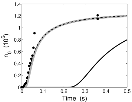
FIG. 11.: A comparision between the data of Fig. 4 of [11] (large solid dots) and our own calculations. The solid curve shows the growth curve for the static parameters that we have extracted from the experimental data: $N_{i}=40\times 10^{6}$, $T_{i}=945.5$nK, $\eta=2.19$. An apparent fit can also be obtained—the parameters for the grey curve (our results) and dashed curve (Bijlsma et al.) are $N_{i}=40\times 10^{6}$ atoms, $T_{i}=765$nK, $\eta=0.6$. However, as noted in the text, these parameters are not experimentally acceptable.

However, while the fit to the experimental data looks very good, the initial parameters for these calculations are not consistent with the experiment. An inspection of the final state of the gas explains the situation. The final temperature according to these computations is $T_{f}=211$nK, and the condensate fraction is 51%. Looking at the data of [11], we find no reported temperatures to be lower than 500nK, and the largest condensate fraction reported to be 30% (although our analysis of their data from Fig. 5 gave a maximum of 17%). The evaporative cooling of these particular simulations would have to remove 94% of the atoms in the trap, and we believe it is very unlikely that this matches any of the experimental situations.

3 Speedup of condensate growth compared to simplified theory

We have shown that a significant speedup of the condensate growth can occur at higher condensate fractions, but this cannot explain this particular discrepancy with the experimental results, for all of the measured values of temperature and condensate fraction for which growth rates are presented in Fig. 5 of [11].

The only situation in which this speedup might possibly be relevant to experiment is the single growth curve corresponding to Fig. 10. However, as we have noted, the initial conditions for this figure are quite speculative, and in fact also appear to be unrealistic.

The actual speedup observed in our computations is of the order of magnitude of that achievable with a different condensate fraction, and it is conceivable that the problem could be experimental rather than theoretical—a systematic error in the methodology of extracting the condensate number from the observed data could possibly cause the effect. For a realistic comparison to be made between experiment and theory, sufficient data should be taken to verify positively all the relevant parameters which have an influence on the results. Thus, one should measure initial and final temperatures, the final condensate number, the number of atoms in the vapor initially and finally, and the size of the “cut”. It should be noted in particular, in the one case where all of this data is available—that presented in Fig. 11—good agreement is not found.

The previous paper in this series, QKVI, considered in detail a semi-classical method of fitting theoretical spatial distributions to the two dimensional data extracted by phase-contrast imaging of the system during condensate growth. This method shows that significantly different condensate numbers and temperatures are consistent with the MIT data and methodology [11]. This seems to us to be a more likely origin of the discrepancy between theory and experiment at low temperatures with a small condensate number.

H Outlook

It does remain conceivable, however, that approximations made in this formulation of Quantum Kinetic theory are not appropriate to the experimental regime where the discrepancy remains. In this section we summarise the possible further extensions.

The first is the ergodic approximation, that all levels of a similar energy are assumed to be equally occupied. From the results of QKII it would seem than any non-ergodicity in the initial distribution would be damped on the time-scale of the growth—therefore the effect of this could be significant if the initial distribution is far from ergodic. It is difficult to know what the exact initial distribution of the system is without performing a three-dimensional detailed calculation of the evaporative cooling, which would require massive computational resources. There is also the fact that we have used the simplified form (22), derived in analogy with the work of Holland et al. [13] on the ergodic approximation.

The second important approximation is that the lower-lying states of the gas are reasonably well described by the single particle excitation spectrum, and thus using a density of states description in calculating the collision rates of these levels. The justification of this is that these states are not expected to be important in determining the growth of the condensate, and in QKVI it was shown that varying these rates by orders of magnitude had little effect on the growth curves.

A third approximation made is that the growth of the condensate level is adiabatic, and its shape remains well described by the Thomas-Fermi wave function. This may not be the case, and indeed some collective motion during growth was observed in [11]. We feel this may become important for sufficiently large truncations of the thermal cloud, in experiments that could be considered a temperature “quench”. Removing this assumption would require introducing a full description of the lower lying quasiparticle levels, and a time dependent Gross-Pitaevskii equation for the shape of the condensate.

The final approximation is that fluctuations of the occupation of the quantum levels are ignored.

The agreement between the theory and the single experiment performed so far is generally good, and there is only one regime in which there is significant discrepancy. The removal of these approximations requires a large amount of work, and we feel this is not justified until new experimental data on condensate growth becomes available.

VI Conclusion

We have extended the earlier models of condensate growth [1, 2, 3] and QKVI to include the full time-dependence of both the condensate and the thermal cloud. We have compared the results of calculations using the full model with the simple model, and determined that for bosonic stimulation type experiments resulting in a condensate fraction of the order of 10%, the model of [3] and QKVI is quite sufficient.

However, for larger condensate fractions the depletion of the thermal cloud becomes important. We have introduced the concept of the effective chemical potential $\mu_{\rm eff}$ for the thermal cloud as it relaxes, and observed it to overshoot its final equilibrium value in these situations, resulting in a much higher growth rate than the simple model would predict. Thus we have identified a mechanism for a possible speedup that may contribute to eliminating the discrepancy with experiment.

We have also found that the results of these calculations can be qualitatively explained using the effective chemical potential of the thermal cloud, $\mu_{\rm eff}$, and the simple growth equation (1). In particular, the rate of condensate growth for the same size condensate can be remarkably similar over a wide range of temperatures; in contrast, the rate of growth is highly sensitive to the final condensate number at a fixed temperature.

This model we have used in this paper eliminates all the major approximations in the calculation of condensate growth, apart from the ergodic assumption, whose removal would require massive computational resources. In the absence of experimental data sufficiently comprehensive to make possible a full comparison between experiment and theory, this does not at present seem justified.

In Sect. V G 2 we have compared the results of our simulations to those of Bijlsma et al. [17], and found that our formulations are quantitatively very similar, giving growth curves in very good agreement with each other. The two treatments are based on similar, but not identical methodologies, and have been independently computed. Thus the disagreement with experiment must be taken seriously.

REFERENCES

- [1] C. W. Gardiner, P. Zoller, R. J. Ballagh and M. J. Davis, Phys. Rev. Lett. 79, 1793 (1997)
- [2] C. W. Gardiner, M. D. Lee, R. J. Ballagh M. J. Davis and P. Zoller, cond-mat/9801027 (1998)
- [3] C. W. Gardiner, M. D. Lee, R. J. Ballagh, M. J. Davis, and P. Zoller, Phys. Rev. Lett. 81, 5266 (1997)
- [4] In this paper will use the notation: QKI for [5], QKII for [6], QKIII for [7], and QKIV for [8] QKV for [9] QKVI for [10]
- [5] C.W. Gardiner and P. Zoller, Phys. Rev. A 55, 2902 (1997)
- [6] D. Jaksch, C.W. Gardiner and P. Zoller, Phys. Rev. A 56, 575 (1997)
- [7] C.W. Gardiner and P. Zoller, Phys. Rev. A 58, 536 (1998)
- [8] D. Jaksch, C.W. Gardiner and P. Zoller, Phys. Rev. A 58, 1450 (1997)
- [9] C.W. Gardiner and P. Zoller, Phys. Rev. A 61, 033601 (2000)
- [10] M. D. Lee and C. W. Gardiner, Quantum Kinetic Theory VI: The Growth of a Bose-Einstein Condensate, cond-mat/9912420, Phys. Rev. A in press
- [11] H. J. Miesner, D. M. Stamper-Kurn, M. R. Andrews, D. S. Durfee, S. Inouye, and W. Ketterle, Science 279, 1005 (1998)
- [12] F. Dalfovo, S. Giorgini, L.P. Pitaevskii and S. Stringari, Rev. Mod. Phys. 71, 463 (1999)
- [13] M. Holland, J. Williams, J. Cooper, Phys. Rev. A 55, 3670 (1997)
- [14] E. Timmermans, P. Tommasini, and K. Huang, Phys. Rev. A. 55, 3645 (1997)
- [15] W. H. Press, S. A. Teukolsky, W. T. Vetterling, and B. P. Flannery, Numerical Recipes in C (Cambridge University Press, Cambridge, 1992)
- [16] O. J. Luiten, M. W. Reynolds, and J. T. M. Walraven, Phys. Rev. A 53, 381 (1996); M.J. Davis, B.Sc. Honours thesis, University of Otago (1996).
- [17] M. Bijlsma, E. Zaremba, and H. T. C. Stoof cond-mat/0001323 (2000)