To appear in the proceedings of SIGIR 2001

Iterative Residual Rescaling:
An Analysis and Generalization of LSI

Abstract

We consider the problem of creating document representations in which inter-document similarity measurements correspond to semantic similarity. We first present a novel subspace-based framework for formalizing this task. Using this framework, we derive a new analysis of Latent Semantic Indexing (LSI), showing a precise relationship between its performance and the uniformity of the underlying distribution of documents over topics. This analysis helps explain the improvements gained by Ando’s (2000) Iterative Residual Rescaling (IRR) algorithm: IRR can compensate for distributional non-uniformity. A further benefit of our framework is that it provides a well-motivated, effective method for automatically determining the rescaling factor IRR depends on, leading to further improvements. A series of experiments over various settings and with several evaluation metrics validates our claims.

1 Introduction

Background

The rapid increase in the availability of electronic documents has created high demand for automated text analysis technologies such as document clustering, summarization, and indexing. Representations enabling accurate measurement of semantic similarities between documents would greatly facilitate such technologies. In this paper, we focus on representations in which vector directionality is used to represent a document’s semantics, by which we mean its (human-interpretable) constituent concepts. This goal is to be accomplished without access to concept labels, since they are typically not available in many applications.

The vector space model (VSM) is a classic method for constructing such vector-based representations. It encodes a document collection by a term-document matrix whose $[i,j]$th element indicates the association between the $i$th term and $j$th document. However, as has been pointed out previously, VSM does not always represent semantic relatedness well; for instance, documents that do not share terms are mapped to orthogonal vectors even if they are clearly related.

Latent Semantic Indexing (LSI) [Deerwester et al.1990, Dumais1991] attempts to overcome this and other shortcomings by computing an approximation to the original term-document matrix; this is equivalent to projecting the term-document matrix onto a lower-dimensional subspace. LSI has been successfully applied to information retrieval and many language analysis tasks (e.g. Dumais+Nielsen:92a, Foltz+Dumais:92a, Berry:95a, Foltz+Kintsh+Landauer:98a, and Wolfe+al:98a), prompting several studies to explain its effectiveness (e.g. Bartell+al:92a, Story:96a, Ding:99a, Papadimitriou+al:00a, and Azar+al:01a).

Ando:00L introduced an alternative subspace-projection method, which we call Iterative Residual Rescaling (IRR), that outperforms LSI by counteracting its tendency to ignore minority-class documents. This is done by repeatedly rescaling vectors to amplify the presence of documents poorly represented in previous iterations. However, Ando presented only heuristic arguments to explain IRR’s success.

Contributions

In this paper, we use the notion of subspace projection to formalize the document representation problem. Based on this framework, we provide a new theoretical analysis that shows a precise relationship between the performance of LSI and the uniformity of the underlying distribution of documents over topics. As a consequence, we provide an explanation for IRR’s success: the rescaling it performs compensates for non-uniformities in the topic-document distribution. Moreover, our framework yields a new way to automatically adjust the amount of rescaling by estimating the non-uniformity.

To support our theoretical results, we present performance measurements both on document sets in which the topic-document distributions were carefully controlled, and on unrestricted datasets as would be found in application settings. In all cases and for all metrics, the results confirm our theoretical predictions. For instance, IRR combined with our new parameter selection technique achieved up to 10.1% higher kappa average precision than LSI and up to 8.7% better document clustering performance. The experiments as a whole provide strong evidence for the usefulness of our framework in general and the effectiveness of our augmented IRR in particular.

Notational conventions

A bold uppercase letter (e.g. $\mathbf{M}$) denotes a matrix; the corresponding bold lowercase letter with subscript $i$ (e.g. $\mathbf{m}_{i}$) denotes the matrix’s $i$th column vector. We use ${\rm range}(\mathbf{M})$ to denote $\mathbf{M}$’s range, or column space: $\{\mathbf{y}~{}|~{}\exists\mathbf{x}\mbox{ such that }\mathbf{y}=\mathbf{M}\mathbf{x}\}$. When a document collection has been specified, $n$ denotes the number of documents the collection contains.

2 Analyzing LSI

2.1 Topic-based similarities

Our framework for analyzing Latent Semantic Indexing and other subspace-based methods revolves around the notion of topic-based similarity. Fix an $n$-document collection ${\cal C}$ and corresponding $m$-by-$n$ term-document matrix $\mathbf{D}$. We assume that there exists a set, denoted ${\rm topics}({\cal C})$, of $k<n$ topics underlying ${\cal C}$. We also assume that for each topic $t$ and document $d$ there exists a (real-valued) relevance score $\mbox{rel}(t,d)$, suitably normalized so that for each $d$, we have $\sum_{t\in{\rm topics}({\cal C})}{\mbox{rel}(t,d)}^{2}=1$. We then define the true topic-based similarity between two documents $d$ and $d^{\prime}$ as:

$${\rm sim}(d,d^{\prime})=\sum_{t\in{\rm topics}({\cal C})}\mbox{rel}(t,d)\mbox{rel}(t,d^{\prime})\,.$$

It is convenient to summarize these similarities in a single $n$-by-$n$ matrix $\mathbf{S}$, where $\mathbf{S}[d,d^{\prime}]={\rm sim}(d,d^{\prime})$.

Note that although we assume the existence of underlying topics as the basis for the true document similarities, in contrast to other analyses (e.g. Papadimitriou+al:00a, Azar+al:01a, and Ding:99a) we do not assume that there is an underlying generative or probabilistic model that creates the term-document matrix $\mathbf{D}$.

2.2 The optimum subspace

We formulate the ultimate goal of subspace-based algorithms, such as LSI, as choosing some subspace such that projecting $\mathbf{D}$ onto this subspace creates new document vectors whose measured similarities (i.e., cosines) more closely correspond to the true topic-based similarities.

More formally, for any subspace ${\cal X}\subseteq\Re^{m}$, the unique (orthogonal) projection of a vector $\mathbf{x}\in\Re^{m}$ onto ${\cal X}$ is given by $\mathbf{P}_{{\cal X}}(\mathbf{x})=\mathbf{B}\mathbf{B}^{T}\mathbf{x}$ for any $\mathbf{B}$ whose columns form an orthonormal basis for ${\cal X}$. We define the projection of $\mathbf{D}$ onto ${\cal X}$ as the matrix $\left[\matrix{\mathbf{P}_{{\cal X}}(\mathbf{d}_{1})\cdots\mathbf{P}_{{\cal X}}(\mathbf{d}_{n})}\right]$, i.e., the result of projecting each of the term-document vectors. Hence, after projection onto ${\cal X}$, the similarity between the $i$th and $j$th documents is measured by

$$\cos(\mathbf{P}_{{\cal X}}(\mathbf{d}_{i}),\mathbf{P}_{{\cal X}}(\mathbf{d}_{j}))=\frac{\mathbf{P}_{{\cal X}}(\mathbf{d}_{i})^{T}\mathbf{P}_{{\cal X}}(\mathbf{d}_{j})}{|\mathbf{P}_{{\cal X}}(\mathbf{d}_{i})||\mathbf{P}_{{\cal X}}(\mathbf{d}_{j})|}\,.$$

The document representation problem is as follows: given $\mathbf{D}$ — but not $\mathbf{S}$ or even any knowledge of what the underlying topics are — find a subspace ${\cal X}$ such that the entries of the deviation matrix

$${\mbox{diff}_{\mathbf{S},\mathbf{D}}}({\cal X})=\mathbf{S}-\mathbf{P}_{{\cal X}}(\mathbf{D})^{T}\mathbf{P}_{{\cal X}}(\mathbf{D})$$

are small. The optimum subspace

$${\cal X}_{opt}=\mathop{\arg\min}_{{\cal X}\subseteq{\rm range}(\mathbf{D})}||{\mbox{diff}_{\mathbf{S},\mathbf{D}}}({\cal X})||_{2}\,,$$

with ties broken by smallest dimensionality and then arbitrarily, serves as the standard for comparison in our analysis. We denote the corresponding projection operator by $\mathbf{P}_{opt}$, and use ${\epsilon_{opt}}$ to denote the optimum error $||{\mbox{diff}_{\mathbf{S},\mathbf{D}}}({\cal X}_{opt})||_{2}$. Note that ${\epsilon_{opt}}$ need not be zero, as it may be impossible to project the given term-document matrix in such a way as to perfectly recover the true document similarities.

2.3 The singular value decomposition and LSI

In this section, we first briefly introduce the singular value decomposition (SVD) [Golub and Van Loan1996], since singular values are necessary for our analysis. Then, we describe LSI, which is based on the SVD.

The SVD factors an arbitrary rank-$h$ matrix $\mathbf{Z}\in\Re^{r\times s}$ into the following product:

$$\mathbf{Z}=\mathbf{U}\mathbf{\Sigma}\mathbf{V}^{T}\,,$$

where the columns of $\mathbf{U}\in\Re^{r\times h}$ and $\mathbf{V}\in\Re^{s\times h}$ are orthonormal, $\mathbf{\Sigma}=\mbox{diag}(\sigma_{1},\sigma_{2},\ldots,\sigma_{h})$ is diagonal (following convention, we assume $\sigma_{1}\geq\cdots\geq\sigma_{h}$), and the $\sigma_{i}$’s are all positive. The quantities $\sigma_{i}$, $\mathbf{u}_{i}$ and $\mathbf{v}_{i}$ are called the $i$th singular value, left singular vector, and right singular vector, respectively. The left singular vectors span $\mathbf{Z}$’s range, and $\sigma_{1}=||\mathbf{Z}||_{2}$.

Zeroing out all but the $\ell<h$ largest singular values yields the least-squares optimal rank-$\ell$ approximation to $\mathbf{Z}$. Latent Semantic Indexing (LSI) [Deerwester et al.1990, Dumais1991] applies this rank-$\ell$ approximation to the term-document matrix $\mathbf{D}$, which corresponds to projecting $\mathbf{D}$ onto the rank-$\ell$ LSI subspace spanned by $\mathbf{u}_{1},\ldots,\mathbf{u}_{\ell}$: letting $\mathbf{U}_{\ell}=\left[\matrix{\mathbf{u}_{1}\ldots\mathbf{u}_{\ell}}\right]$,

$$\mathbf{U}_{\ell}\mathbf{U}_{\ell}^{T}\mathbf{D}=\mathbf{U}\;\mbox{diag}(\underbrace{\sigma_{1},\cdots,\sigma_{\ell},0,\cdots,0}_{h\mbox{ entries}})\;\mathbf{V}^{T}.$$

Note that the fact that this matrix approximates $\mathbf{D}$ well does not imply that it represents the true document similarities well, as we shall see.

Further intuition may be gained on the left singular vectors by the following observation. Let ${\rm proj}^{(j)}(\mathbf{d}_{i})$ be the projection of $\mathbf{d}_{i}$ onto the span of $\mathbf{u}_{1},\ldots,\mathbf{u}_{j}$, and let $\mathbf{r}_{i}^{(j)}$ be the residual vector $\mathbf{d}_{i}-{\rm proj}^{(j-1)}(\mathbf{d}_{i})$. Then, $\mathbf{u}_{j}$ is the unit vector that maximizes the following quantity:

$$g^{(j)}(\mathbf{x})=\sum_{i=1}^{n}\left(|\mathbf{r}_{i}^{(j)}|\cos(\mathbf{r}_{i}^{(j)},\mathbf{x})\right)^{2}\,.$$

In a sense, $\mathbf{u}_{j}$ resembles a weighted average of residual vectors, where longer residuals receive greater weight. Hence, the $\ell$ left singular vectors may be thought of as representing the $\ell$ major directions in the document collection.

2.4 Non-uniformity and LSI

We now state our results relating the non-uniformity of the underlying topic-document distribution to the quality of the document representation spaces derived using LSI. The main outline of our argument is to first show relations between certain singular values and certain quantities linked to our topic model, and then show how the distance between the LSI-subspace and the optimal subspace relates to these singular values. Proofs of these results, which make use of invariant subspace perturbation theorems [Davis and Kahan1970, Stewart and Sun1990, Golub and Van Loan1996], are sketched in the appendix of this paper and given in full in Ando:thesis.

Recall that we are dealing with a fixed document collection ${\cal C}$ with $k$ underlying topics. Throughout, we use $h$ to denote the dimensionality of the optimum subspace. For clarity, we will abuse notation by writing “$x\in y\pm z$” as shorthand for “$x\in[y-z,y+z]$”.

A crucial quantity in our analysis is the dominance $\Delta_{t}$ of a given topic $t$:

$$\Delta_{t}=\sqrt{\sum_{d\in{\cal C}}\mbox{rel}(t,d)^{2}}\,.$$

(It may be helpful to observe that in the special “single-topic documents” case, where each document is relevant to only one topic in ${\rm topics}({\cal C})$, squaring $\Delta_{t}$ gives exactly the number of documents in ${\cal C}$ that are relevant to topic $t$.) We assume without loss of generality that $\Delta_{1}\geq\Delta_{2}\geq\cdots\geq\Delta_{k}$, and for convenience set $\Delta_{i}=0$ if $i>k$.

Now we show that the projection of $\mathbf{D}$ onto the optimum subspace ${\cal X}_{opt}$ in some sense reveals the topic dominances. It is intuitively clear, however, that the extent to which this holds should depend to some degree both on the optimum error ${\epsilon_{opt}}$ and on the topic mingling $\mu({\cal C})=\left(\sum_{t,t^{\prime}\in{\rm topics}({\cal C}),t\neq t^{\prime}}\left(\sum_{d\in{\cal C}}\mbox{rel}(t,d)\mbox{rel}(t^{\prime},d)\right)^{2}\right)^{1/2}$ (note that in the single-topic documents case, $\mu({\cal C})=0$). Certainly, if the optimum error is high, then we cannot expect the optimum subspace to fully reveal the topic dominances; also, if there is high topic mingling in the collection, then the topics will be fairly difficult to distinguish.

Theorem 2.1

Let $\tau_{i}$ be the $i$th largest singular value of $\mathbf{P}_{opt}(\mathbf{D})$. Then, $\tau_{i}^{2}\in\Delta_{i}^{2}\pm({\epsilon_{opt}}+\mu({\cal C}))$.

This result gives us leave to define $\widehat{\Delta}_{max}=\tau_{1}$ and $\widehat{\Delta}_{min}=\tau_{h}$, where $h$ is the dimension of ${\cal X}_{opt}$. The ratio $\widehat{\Delta}_{max}/\widehat{\Delta}_{min}$ then serves as a measure of the non-uniformity of the topic-document distribution underlying the collection: the more the largest topic dominates the collection, the higher this ratio will tend to be.

Now we are in a position to present our main theorem. This result bounds the distance between the optimum subspace ${\cal X}_{opt}$ and the same-dimensionality LSI subspace ${\cal X}_{LSI}$ by a function of the non-uniformity of ${\cal C}$’s topic-document distribution. The bound also incorporates a certain value (defined precisely in the appendix) $\widehat{\epsilon}_{vsm}\in\epsilon_{vsm}\pm{\epsilon_{opt}}$, where $\epsilon_{vsm}=||{\mbox{diff}_{\mathbf{S},\mathbf{D}}}({\cal X}_{VSM})||_{2}=||\mathbf{S}-\mathbf{D}^{T}\mathbf{D}||_{2}$ is the input error: intuitively, if a “bad” term-document matrix is received as input, one cannot expect LSI to do well.

Theorem 2.2

Let ${\cal X}_{LSI}$ be the $h$-dimensional LSI subspace spanned by the the first $h$ left singular vectors of $\mathbf{D}$. If $\widehat{\Delta}_{min}>\sqrt{\widehat{\epsilon}_{vsm}}$, then

$$||\tan(\Theta({\cal X}_{LSI},{\cal X}_{opt}))||_{2}\leq\frac{\widehat{\Delta}_{max}}{\widehat{\Delta}_{min}}\cdot\frac{\sqrt{\widehat{\epsilon}_{vsm}}/\widehat{\Delta}_{min}}{1-(\sqrt{\widehat{\epsilon}_{vsm}}/\widehat{\Delta}_{min})^{2}}\,,$$

where $\Theta$ is the canonical angle matrix measuring the distance between subspaces [Davis and Kahan1970, Stewart and Sun1990].

Intuitively, what this means is that ${\cal X}_{LSI}$ must be close to ${\cal X}_{opt}$ when the topic-document distribution is relatively uniform and the input error is small in comparison to the $h$th largest topic dominance. Conversely, if the input error is fixed, our bound on LSI’s performance weakens when the underlying topic-document distribution is highly non-uniform. Finally, we note that the condition on $\widehat{\epsilon}_{vsm}$ is natural: roughly speaking, if the input error is large enough to “swamp” the dominance of the $h$th largest topic, then intuitively we cannot expect good results.

Finally, we note that a related result can be proved which, roughly speaking, links lower bounds on the distance between the two subspaces to non-uniformity and the input error; however, this theorem is quite technical in nature and thus is omitted. We refer the reader to Ando:thesis for details.

2.5 Related work: theoretical analyses of LSI

As noted above, there have been several studies analyzing LSI, using approaches such as Bayesian regression models [Story1996] and Gaussian models [Ding1999]. Here, we concentrate on describing the work most similar in spirit to ours.

Zha+Marques+Simon:98a propose a subspace-based model for LSI. Their work focuses on dimensionality selection and implementation issues regarding more accurate updating schemes. Bartell+al:92a show that LSI can be regarded as a solution to the special Multidimensional Scaling (MDS) problem of preserving the inner products of the original document vectors. However, as noted above, this is not the same as recovering hidden topic-based similarities, especially in the case of noisy data.

Perhaps the work most similar to ours is that of Papadimitriou+al:00a and Azar+al:01a, both of which propose to explain LSI’s success with analyses that, like ours, employ invariant subspace perturbation theorems. Papadimitriou et al. start with a probabilistic corpus model. By assuming low input error and certain conditions on singular values (which, from our perspective, can be considered to be roughly equivalent to assuming relative uniformity, although Papadimitriou et al. did not explicitly make this connection), they show that LSI will work well with high probability. But their results are based on a pure probabilistic corpus model in which all the documents are single-topic and topics have associated primary (distinguishing) disjoint sets of terms. Thus, their analysis holds only for a very restricted class of document collections. Similarly, Azar et al. also start with particular conditions and a specialized underlying generative model to show that LSI works well for “good” documents with high probability. In contrast to these approaches, our analysis does not assume a model of term-document matrix creation, and so applies to arbitrary term-document matrices, with the non-uniformity and the input matrix’s quality being explicit terms in our bound.

3 IRR: Overcoming non-uniformity

Our results from Section 2.4 indicate that we could improve the performance of LSI if we could somehow “smooth” the topic-document distribution (that is, effectively lower $\widehat{\Delta}_{max}/\widehat{\Delta}_{min}$). We show that the Iterative Residual Rescaling (IRR) algorithm, introduced (but not named) and heuristically motivated by Ando:00L, accomplishes this task without prior knowledge of the assignments of documents to topics.

3.1 Ando’s IRR algorithm

Figure 1: Effect of nonuniformity on LSI, and how IRR compensates.

IRR	$(q,$	$\ell)$:
	$\mathbf{R}$:= $\mathbf{D}$     /* initialize residuals by given $m$-by-$n$ term-document matrix */
	For $j:=1,2,\ldots,\ell~{}~{}~{}~{}$ /* create $\ell$ basis vectors */
		For $i:=1,2,\ldots,n$
			${\hat{\mathbf{r}}_{i}}:=|\mathbf{r}_{i}|^{q}\mathbf{r}_{i}~{}~{}~{}~{}$ /* rescale residuals */
		$\mathbf{b}_{j}:=\arg\max_{\mathbf{x}:|\mathbf{x}|=1}\left(\sum_{i=1}^{n}\left(|{\hat{\mathbf{r}}_{i}}|\cos(\hat{\mathbf{r}}_{i},\mathbf{x})\right)^{2}\right)$
		For $i:=1,2,\ldots,n$
			Subtract from $\mathbf{r}_{i}$ its projection onto $\mathbf{b}_{j}$     /* recompute residuals */
	$\mathbf{D}_{\mbox{IRR}}:=\mathbf{B}\mathbf{B}^{T}\mathbf{D}$, where $\mathbf{B}=\left[\matrix{\mathbf{b}_{1}&\mathbf{b}_{2}&\cdots&\mathbf{b}_{\ell}}\right]$ /* new document representation */

Figure 2: High-level pseudocode for Ando’s IRR (i.e. before augmentation with auto-scale).

Recall from Section 2.3 that the left singular vectors $\mathbf{u}_{1},$ $\mathbf{u}_{2},\ldots$ produced by LSI can be derived, one by one, via the following computation:

$$\mathbf{u}_{j}=\mathop{\arg\max}_{|\mathbf{x}|=1}\sum_{i=1}^{n}\left(|\mathbf{r}_{i}^{(j)}|\cos(\mathbf{r}_{i}^{(j)},\mathbf{x})\right)^{2},$$

where the $\mathbf{r}_{i}^{(j)}$ are the residuals $\mathbf{d}_{i}-{\rm proj}^{(j-1)}(\mathbf{d}_{i})$. Unfortunately, inspection of this formula shows that when the topic-document distribution is highly non-uniform, the cumulative influence of a large number of (small) residuals for a major topic can cause smaller topics to be ignored, as depicted in Figures 1(a) and (b).

Our explanation of IRR’s effectiveness is that by amplifying the length differences among residual vectors, IRR boosts the influence of minority-topic documents, thus compensating for non-uniform topic distributions (Figure 1(c)). More precisely, IRR, like (our formulation of) the SVD, computes basis vectors by successive maximizations, as shown in the pseudocode in Figure 2. Crucially, though, IRR’s objective function, $\widehat{g}^{(j)}$, incorporates a scaling factor $q$ via the scaling function ${\rm pow}(\mathbf{r},q)=|\mathbf{r}|^{q}~{}\mathbf{r}$:

$$\widehat{g}^{(j)}(\mathbf{x})=\sum_{i=1}^{n}\left(|{\rm pow}(\mathbf{r}_{i}^{(j)},q)|~{}\cos({\rm pow}(\mathbf{r}_{i}^{(j)},q),\mathbf{x})\right)^{2}\,.$$

This is maximized by the first left singular vector of

$$\widehat{\mathbf{R}}^{(j)}=\left[\matrix{{\rm pow}(\mathbf{r}_{1}^{(j)},q)&\cdots&{\rm pow}(\mathbf{r}_{n}^{(j)},q)}\right]\,.$$

That is, IRR rescales each residual vector $\mathbf{r}_{i}$ at each basis vector computation, increasing the contrast between long and short residuals when $q>0$. LSI is the special case in which $q=0$.

3.2 The AUTO-SCALE method

Our discussion above argues that the degree of rescaling should depend on the uniformity of the topic-document distribution. Ando:00L did not explicitly make this connection, and hence could not take advantage of it: $q$ was determined simply by training on held-out data. In contrast, our novel analysis allows us to exploit this connection to develop an effective estimation method — automatic scaling factor determination (auto-scale) — that approximates the topic-document non-uniformity without prior knowledge of the underlying topics.

auto-scale is based on the observation that we can use the quantity $\sum_{t\in{\rm topics}({\cal C})}\Delta_{t}^{4}/n^{2}$ as a measure of the non-uniformity of the topic-document distribution. Of course, we don’t have access to the topic dominances $\Delta_{t}$, but we can approximate this measure by

$$f(\mathbf{D})\stackrel{{\scriptstyle def}}{{=}}\left(\frac{||\mathbf{D}^{T}\mathbf{D}||_{F}}{n}\right)^{2}\,.$$

This approximation follows from first assuming that the input matrix is fairly good, so that $||\mathbf{D}^{T}\mathbf{D}||_{F}^{2}$ is roughly equal to $||\mathbf{S}||_{F}^{2}=\sum_{d,d^{\prime}\in{\cal C}}\left(\sum_{t\in{\rm topics}({\cal C})}\mbox{rel}(t,d)\mbox{rel}(t,d^{\prime})\right)^{2}$. The latter can be rewritten, after some algebra, as the quantity $\sum_{t\in{\rm topics}({\cal C})}\Delta_{t}^{4}+\mu({\cal C})^{4}$, which is roughly $\sum_{t\in{\rm topics}({\cal C})}\Delta_{t}^{4}$ if we assume approximately single-topic documents. In practice, we set $q$ to a linear function of $f(\mathbf{D})$; this is discussed in Section 5.1.

Although the above assumptions are rather coarse, auto-scale yields good empirical results: see Sections 5 and 6.

3.3 Dimensionality selection

IRR’s second parameter is $\ell$, the dimensionality of the created subspace. One way to set this parameter is to train it on held-out data. Following Ando:00L, we found that learning thresholds on the residual ratio $||\mathbf{R}^{(j)}||_{F}^{2}/n$ as a stopping criterion is effective for both LSI and IRR. Intuitively, this ratio describes how much is left out of the proposed subspace (of course, we do not want to reproduce the term-document matrix exactly — hence the threshold). Note that this training method allows some flexibility in the chosen dimensionality: for different data sets, the same residual ratio threshold may result in selecting a different $\ell$.

While training on held-out data is reasonable and is commonly employed in practice, it is a relatively expensive process. A speedier alternative arises in settings in which $k$, the number of topics, is pre-specified — examples include cases where the topic set is a fixed class such as the TREC topic labels, or where the application allows the user to specify the appropriate level of granularity for his or her needs. In such settings, we could simply set the dimensionality equal to $k$ as a matter of convenience. (Indeed, Papadimitriou+al:00a show that under certain strong assumptions on the data, rank-$k$ LSI should perform well. See also Ando:thesis.) We describe experiments with both selection methods below.

4 Evaluation metrics

Kappa average precision   Our first evaluation metric is based on the pair-wise average precision [Ando2000], adapted from the average precision measure commonly used in information retrieval. The motivation behind this metric is that the measured similarity for any two intra-topic documents (i.e., that share at least one topic) should be higher than for any two cross-topic documents which have no topics in common. More formally, let $p_{i}$ denote the document pair with the $i$th largest measured similarity (cosine). Precision for an intra-topic pair $p_{j}$ is defined by

$${\rm prec}(p_{j})=\frac{\#\mbox{ of intra-topic pairs $p_{i}$ such that $i\leq j$}}{\mbox{$j$}}\,.$$

The pair-wise average precision is the average of these precision values over all intra-topic pairs.

To compensate for the effect of large topics (which increase the likelihood of chance intra-topic pairs), we modify the pair-wise average precision to create a new metric, which we call the kappa precision in reference to the Kappa statistic [Siegel and Castellan, Jr.1988, Carletta1996]:

$${\rm prec}_{\kappa}(p_{i})=\frac{{\rm prec}(p_{i})-{\rm chance}}{1-{\rm chance}}\,,$$

where ${\rm chance}=$ ($\#$ of intra-topic pairs)/($\#$ of document pairs). The kappa average precision $\kappa$ is defined to be the average of the kappa precision over all intra-topic pairs, and is a linear function of the pair-wise average precision.

Clustering   We also test how well the new subspaces represent document similarities by seeing whether document clustering improves when these new representations are used as input. To simplify the scoring, we consider only single-topic documents.

Let $C$ be a cluster-topic contingency table such that $C[i,j]$ is the number of documents in cluster $i$ that are relevant to topic $j$, as in Slonim+Tishby:00a. We define $s(C)=\sum_{i,j}{\cal N}_{ij}/n$, where ${\cal N}_{ij}=C[i,j]$ if $C[i,j]$ is the unique maximum in both its row and column, and ${\cal N}_{ij}=0$ otherwise. Note that this (rather strict) measure only considers the most tightly coupled topic-cluster assignment, and decreases when either cluster purity or topic integrity declines (see Figure 3).

	topic 1	topic 2	topic 3	topic 4
cluster 1	5	10	20	0
cluster 2	5	10	5	0
cluster 3	0	0	0	21
cluster 4	15	5	0	0
cluster 5	0	0	0	4

Figure 3: Sample contingency table, with $s(C)=(15+20+21)/100=56\%$.

To factor out the idiosyncracies of particular clustering algorithms, we apply six standard clustering methods — single-link, complete-link, group average, and k-means with initial clusters generated by these three methods — to the document vectors in each proposed subspace, and record both the ceiling (highest) and floor (lowest) $s(C)$ scores. While the ceiling performance is perhaps more intuitive, we observe that the floor performance also gives us important information about the quality of the representation being evaluated: if the floor is low, then there is at least one clustering algorithm for which the document subspace is not a good representation; otherwise, the representation is good for all six clustering algorithms.

5 Controlled distributions

Our first suite of experiments studies the dependence of LSI and IRR on increasingly less uniform topic-document distributions. The results strongly support our theoretical analysis of LSI’s sensitivity to non-uniformity.

5.1 Experimental setting

To focus on distributional non-uniformity, we first chose two TREC topics, and then specified seven distribution types: (25, 25), (30, 20), (35, 15), (40, 10), (43, 7), (45, 5), and (46, 4), where $(n_{1},n_{2})$ indicates that $n_{i}$ of the documents are relevant to topic $i$. For each of these types, we generated ten sets of 50 TREC documents each, where each document was relevant to exactly one of the pre-selected topics. We also created five-topic data sets in the same manner, using distribution types of the form $(i,j,j,j,j)$ (which makes uniformity comparisons obvious).

To create the term-document matrices, we extracted single-word stemmed terms using TALENT [Boguraev and Neff2000], removed stopwords, and then length-normalized the document vectors (so that term weights were frequency-based).

To implement auto-scale, we set $q=\alpha\cdot f(\mathbf{D})+\beta$, where $\alpha=3.5$ and $\beta=0$ for all our experiments. These values (which are necessary to determine the “units” of the scale factor) were empirically determined once and for all from observations on data disjoint from our test sets. This contrasts with training $q$ for every new test set encountered, as in Ando:00L. Training is an expensive process, and we envision interactive applications such as organizing query results (a task we simulate in Section 6) in which what would serve as training data is not obvious. We thus view auto-scale as a practical alternative to the usual parameter training.

For simplicity, the dimensionality of LSI and IRR in our experiments was set to the number of topics.

5.2 Controlled-distribution results

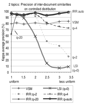
Figure 4: Kappa average performance, two topics. Points are averages over ten document sets.

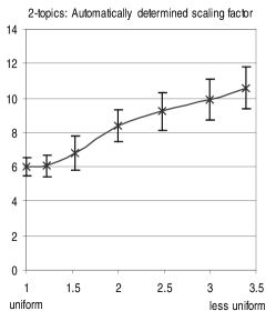
Figure 5: Automatically-determined scaling factor values: ten-set average and standard deviation.

We first examine the kappa average precision results, shown in Figure 4. The $x$-axis represents the nonuniformity of the topic-document distribution, as measured by $\Delta_{max}/\Delta_{min}$. We see that when the topic-document distribution is relatively uniform, LSI’s performance is higher than 90%. However, as the nonuniformity increases, the performance of LSI drops precipitously, in accordance with our theorems above.

Also, our interpretation of the scaling factor $q$ as compensating for non-uniformity is borne out nicely. For highly uniform distributions, the performance difference between $q=0$ (at which IRR = LSI), $q=2$, and $q=4$ is not great. At medium nonuniformity, $q=0$ degrades, but $q=2$ still does about the same as $q=4$. But as the non-uniformity increases even more, we see that $q=2$ is not large enough to compensate, and so declines in comparison to $q=4$.

Furthermore, we see that IRR with auto-scale (labelled ‘IRR:$q={\rm auto}$’) does extremely well across all levels of non-uniformity. Figure 5 shows that auto-scale indeed adjusts for more non-uniform distributions: the chosen scaling factor increases on average as the non-uniformity goes up.

Now, one might conjecture that instead of using auto-scale, it would suffice simply to choose a single very large value of $q$. Intuitively, though, this is problematic, since too high a scaling factor would tend to completely eliminate residuals. Furthermore, the $q=20$ curve in Figure 4 disproves the conjecture: in the uniform case, selecting an overly large scaling factor hurts performance, driving it below the baseline VSM curve.

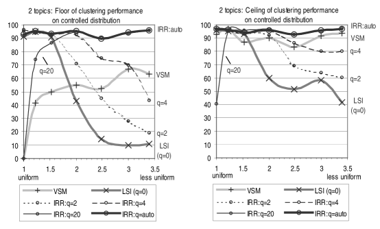
Figure 6: Floor and ceiling clustering results, two topics. Points are averages over ten document sets.

The two-topic floor and ceiling clustering results, shown in Figure 6, exhibit precisely the same types of behaviors as in the kappa average precision case. The floor performances are especially interesting, as they show that auto-scale-IRR exhibits very good performance for all six of our rather wide variety of clustering algorithms. They also indicate that VSM is ‘fragile’ for uniform distributions, in that sometimes it is a very poor representation for at least one of the clustering algorithms we employed.

Finally, Figure 7 shows the results of the same evaluation experiments run on five-topic data. Again, the empirical results are completely in line with what we predicted, with auto-scale leading to strong performance over all metrics and all degrees of non-uniformity. Note that the gap between LSI and VSM decreases in comparison to the $k=2$ case; this is due to the fact that at higher dimensionalities, the subspace produced by LSI gets closer to that of the original term-document matrix.

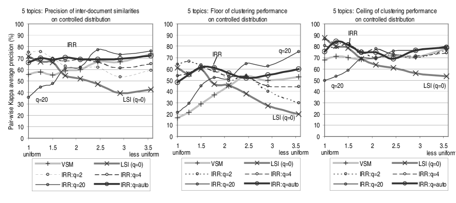
Figure 7: Ten-set averages of kappa average precision and floor and ceiling clustering results, five topics.

These results all strongly support our theoretical claims.

6 Unrestricted distributions

In this section, we experiment on the more realistic setting of document sets without distribution restrictions. We expect that in practice, topic-document distributions will be fairly non-uniform, so that IRR should perform well in comparison to LSI. Figure 8 summarizes the evaluation settings.

We used 648 TREC documents, each relevant to exactly one of twenty TREC topics. To perform parameter training, we randomly divided these documents into two disjoint document pools. We then simulated input from an information retrieval application by generating 15 document sets from each pool, where each set consisted of those documents containing one of 15 arbitrarily chosen keywords; this yielded a total of 30 document sets. Document sets from one pool were used as parameter training data for the sets from the other pool, and vice versa. Performance results are averages over these 30 runs. The scaling factor for IRR was determined by auto-scale in all cases (again with the same constants $\alpha$ and $\beta$ as before). The term-document matrices were created in the same manner as in Section 5.1.

6.1 Kappa average precision results

Recall that we consider two ways to choose the dimensionality of a document subspace. In the first case, the system knows $k$, the number of topics underlying the collection (in practice, this information could be user-supplied as a way to control topic granularity, or given by a set of predetermined classification labels), and sets the dimensionality to it. In the second case, $k$ is considered unknown, so we simply train the dimensionality parameter using the residual ratio method described in Section 3.3.

Metric	$\kappa$		floor/ceiling
Is $k$ given?	yes	no	yes		no
Choice of $\ell$	$k$	train	$k$	train	train
# of clusters	N/A		$k$		$\ell$
Section (Data)	6.1 (Table 9)		6.2 (Figure 10)

Figure 8: Evaluation settings for unrestricted distributions. Recall that $k$ is the number of topics and $\ell$ is the dimensionality.

From Figure 9, we see that IRR yields higher $\kappa$ than LSI and VSM for both dimensionality selection methods, and therefore does a better job at representing inter-document similarities. LSI performs relatively poorly on this task; indeed, using $k$ dimensions in the LSI case leads to worse results than VSM.

Dimensionality selection	LSI	IRR
Number of topics	-8.7	1.4
Trained	0	4.0

Figure 9: Thirty-set average absolute improvement in $\kappa$ over VSM (51.4%), unrestricted distributions.

6.2 Clustering results

To derive floor and ceiling clustering performance results, there are two parameters we need to specify: the dimensionality of the subspace, and the number of clusters.

If $k$, the number of topics, is available, then it is the natural choice for the number of clusters. Then, to choose the dimensionality in this case, one option is to also set it to $k$; Figure 10(a) shows the results. We see that IRR has the best clustering performance overall. Note that LSI’s ceiling is actually lower than VSM’s.

When $k$ is given but we train the dimensionality via the residual ratio, IRR still provides a better subspace for all the clustering algorithms we considered, both in terms of floor and ceiling performance (Figure 10(b)). We observe that for this type of data, training the dimensionality allows LSI to produce improved ceiling results.

We now consider the case in which $k$ is unknown. In this situation, we know of no alternative but to train the dimensionality on held-out data. As for the number of clusters, a reasonable default is to simply set this value to the trained dimensionality. Of course, this doesn’t apply to VSM, since the dimensionality is not a free parameter for it; instead, we set the number of clusters to the average of the number of topics in the training document sets.

Figure 10(c) shows the clustering results for the unknown-$k$ setting. LSI’s ceiling degrades by 4.3% compared with when the number of topics is given, while those of VSM and IRR show almost no change. Furthermore, IRR clearly outperforms the other methods.

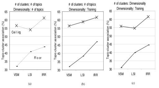
Figure 10: Document clustering performances, unrestricted distributions: averages over 30 runs.

6.3 Discussion

In our experiments, LSI did worse or essentially the same as VSM in 4 out of 8 combinations of practical settings and metrics. In particular, when the dimensionality is chosen to be the number of topics, LSI performs relatively poorly. Dimensionality training improves LSI’s kappa average precision scores, and also improves its clustering performance with respect to VSM as long as the correct number of clusters (i.e. the number of topics) is given. However, when the number of clusters is unknown, LSI’s ceiling clustering performance drops, again indicating that for LSI  the dimensionality should not be tied to the number of clusters.

In contrast, IRR consistently performs better than LSI and VSM for all our settings and metrics. In particular, IRR fares relatively well when the dimensionality is set to the number of topics as compared to when the dimensionality is actually trained. These results suggest that setting the dimensionality to the number of topics, when known, may be a practical alternative to dimensionality training. Furthermore, in clustering applications for which the number of topics is not known, we at least might be able to reduce the training effort by only searching for the dimensionality, setting the number of clusters to the same value.

7 Conclusion

To conclude, we review our three main results. First, we have provided a new theoretical analysis of LSI, showing a precise relationship between LSI’s performance and the uniformity of the underlying topic-document distribution. Second, we have used our framework to extend Ando’s (2000) IRR algorithm by giving a novel and effective method for determining the requisite scaling factor. Third, we have shown that IRR, together with our parameter determination method, provides very good performance in comparison to LSI over a variety of document-topic distributions and applications-oriented metrics.

A Appendix

We use the following perturbation result on singular values, which is a slight rewriting of Corollary 8.6.2 in Golub+VanLoan:96a.

Theorem A.1

Let $\mathbf{E}=\mathbf{X}_{1}-\mathbf{X}_{2}$, where $\mathbf{X}_{1},\mathbf{X}_{2}\in\Re^{r\times s}$ and $r\geq s$, and for $1\leq i\leq s$, let $\sigma_{i}^{(1)}$ and $\sigma_{i}^{(2)}$ denote the $i$th singular values of $\mathbf{X}_{1}$ and $\mathbf{X}_{2}$, respectively. Then,
$|\sigma_{i}^{(1)}-\sigma_{i}^{(2)}|\leq||\mathbf{E}||_{2}\leq||\mathbf{E}||_{F}.$

Notational conventions   If we refer to a singular value $\sigma_{j}$ of a matrix $\mathbf{Z}$ with rank less than $j$, it is understood that $\sigma_{j}=0$. (This corresponds to the “zero-padded” version of the SVD that is also commonly used; we presented the non-padded version above for conceptual clarity.)

Throughout, $\tau_{i}$ denotes the $i$th singular value of $\mathbf{P}_{opt}(\mathbf{D})$.

A.1 Proof of Theorem 2.1

Let $\rho_{1},\ldots,\rho_{n}$ be the singular values of the true topic-based similarities matrix $\mathbf{S}$. For convenience, fix a particular $i\in\{1,\ldots,n\}$.

Since ${\mbox{diff}_{\mathbf{S},\mathbf{D}}}({\cal X}_{opt})=\mathbf{S}-\mathbf{P}_{opt}(\mathbf{D})^{T}\mathbf{P}_{opt}(\mathbf{D})$, by Theorem A.1 we have $\tau_{i}^{2}\in\rho_{i}\pm{\epsilon_{opt}}$.

Next, define the matrix $\mathbf{S}^{\prime}\in\Re^{n\times n}$ by

$$\mathbf{S}^{\prime}[t_{1},t_{2}]=\sum_{d\in{\cal C}}\mbox{rel}(t_{1},d)\mbox{rel}(t_{2},d)\,,$$

where we define $\mbox{rel}(t,d)=0$ for $t>k$ and $d\in{\cal C}$. One can verify that the singular values of $\mathbf{S}^{\prime}$ are the same as the singular values of $\mathbf{S}$: $\rho_{1},\ldots,\rho_{n}$.

Now, consider the matrix $\mathbf{E}\stackrel{{\scriptstyle def}}{{=}}\mathbf{S}^{\prime}-{\rm diag}(\Delta_{1}^{2},\ldots,\Delta_{n}^{2})$. We note that the singular values of ${\rm diag}(\Delta_{1}^{2},\ldots,\Delta_{n}^{2})$ are $\Delta_{1}^{2},\ldots,\Delta_{n}^{2}$. Furthermore, observe that $||\mathbf{E}||_{F}=\mu({\cal C})$, the topic mingling in the collection. Therefore, by again applying Theorem A.1 we find that $\rho_{i}\in\Delta_{i}^{2}\pm\mu({\cal C})$.

Combining our partial results yields the desired result:

$$\tau_{i}^{2}\in\Delta_{i}^{2}\pm({\epsilon_{opt}}+\mu({\cal C}))\,.$$

A.2 Invariant subspace tangent theorem

The proof of Theorem 2.2 is based on the following simplification of the Davis-Kahan tangent theorem [Davis and Kahan1970] (see also Theorem 3.10 of Stewart+Sun:90a).

Theorem A.2

Let $\mathbf{A}\in\Re^{r\times r}$ be a symmetric matrix, and let $\left[\matrix{\mathbf{X}&\mathbf{Y}}\right]$ be an orthogonal matrix, with $\mathbf{X}\in\Re^{r\times p}$, so that ${\rm range}(\mathbf{X})$ forms an invariant subspace of $\mathbf{A}$ (i.e. $\mathbf{x}\in{\rm range}(\mathbf{X})$ implies $\mathbf{A}\mathbf{x}\in{\rm range}(\mathbf{X})$). For any matrix $\widehat{\mathbf{X}}\in\Re^{r\times p}$ with orthonormal columns, we define the residual matrix $\mathbf{R}$ of $\widehat{\mathbf{X}}$ as

$$\mathbf{R}=\mathbf{A}\widehat{\mathbf{X}}-(\widehat{\mathbf{X}}\widehat{\mathbf{X}}^{T})\mathbf{A}\widehat{\mathbf{X}}\,.$$

Suppose the eigenvalues of $\widehat{\mathbf{X}}^{T}\mathbf{A}\widehat{\mathbf{X}}$ lie in the range $[\alpha,\beta]$ and that there exists $\delta>0$ such that the eigenvalues of $\mathbf{Y}^{T}\mathbf{A}\mathbf{Y}$ either all lie in the interval $(-\infty,\alpha-\delta]$ or are all in $[\beta+\delta,\infty)$. Then,

$$||\tan(\Theta({\rm range}(\mathbf{X}),{\rm range}(\widehat{\mathbf{X}}))||_{2}\leq\frac{||\mathbf{R}||_{2}}{\delta}\,.$$

A.3 Proof sketch for Theorem 2.2

Here, we outline the proof (given in full in Ando:thesis). The main idea is to apply Theorem A.2 by choosing $\mathbf{X}$ and $\widehat{\mathbf{X}}$ so that ${\rm range}(\mathbf{X})={\cal X}_{LSI}$ and ${\rm range}(\widehat{\mathbf{X}})={\cal X}_{opt}$, and setting $\mathbf{A}=\mathbf{D}\mathbf{D}^{T}$, for which the LSI subspace is invariant.

Let $\widehat{\mathbf{D}}=\mathbf{P}_{opt}(\mathbf{D})$, and define $\overline{\mathbf{D}}=\mathbf{D}-\widehat{\mathbf{D}}$; note that $\widehat{\mathbf{D}}^{T}\overline{\mathbf{D}}=\overline{\mathbf{D}}^{T}\widehat{\mathbf{D}}=\mathbf{0}$. Let $\sigma_{i}$ denote the $i$th singular value of $\mathbf{D}$.

First, consider the largest singular value of $\overline{\mathbf{D}}^{T}\overline{\mathbf{D}}$, which we will denote by $\widehat{\epsilon}_{vsm}$. It can be shown that $\widehat{\epsilon}_{vsm}\in\epsilon_{vsm}\pm{\epsilon_{opt}}$, thus justifying our choice of notation. (First show that ${\mbox{diff}_{\mathbf{S},\mathbf{D}}}({\cal X}_{opt})={\mbox{diff}_{\mathbf{S},\mathbf{D}}}({\cal X}_{VSM})-(-\overline{\mathbf{D}}^{T}\overline{\mathbf{D}})$, and then apply Theorem A.1 to this equation and observe that the largest singular value of ${\mbox{diff}_{\mathbf{S},\mathbf{D}}}({\cal X}_{VSM})$ is $\epsilon_{vsm}$.)

Then, it can be shown that $\sigma_{h+1}\leq\sqrt{\widehat{\epsilon}_{vsm}}$: apply Theorem A.1 to the equation $\overline{\mathbf{D}}^{T}\overline{\mathbf{D}}=\mathbf{D}^{T}\mathbf{D}-\widehat{\mathbf{D}}^{T}\widehat{\mathbf{D}}$ and then note that $\tau_{h+1}=0$ because of the dimensionality of ${\cal X}_{opt}$.

Now, to apply Theorem A.2, choose the columns of $\mathbf{X}$ to be the first $h$ left singular vectors (in order) of $\mathbf{D}$, and choose the columns of $\widehat{\mathbf{X}}$ to be all $h$ left singular vectors (in order) of $\widehat{\mathbf{D}}$. We set the columns of $\mathbf{Y}$ to the rest of the $m-h$ left singular vectors (in order) of the “zero-padded” version of the SVD of $\mathbf{D}$.

Some linear algebra reveals that the eigenvalues of $\mathbf{Y}^{T}\mathbf{A}\mathbf{Y}$ are no greater than $\sigma_{h+1}^{2}$, and the eigenvalues of $\widehat{\mathbf{X}}^{T}\mathbf{A}\widehat{\mathbf{X}}$ are no smaller than $\widehat{\Delta}_{min}^{2}$. Therefore, we set $\delta=\widehat{\Delta}_{min}^{2}-\sigma_{h+1}^{2}$. Note that $\delta\geq\widehat{\Delta}_{min}^{2}-\widehat{\epsilon}_{vsm}$ by above, and so is positive by assumption. Hence, Theorem A.2 applies.

Finally, it can be shown that $||\mathbf{R}||_{2}\leq\widehat{\Delta}_{max}\cdot\sqrt{\widehat{\epsilon}_{vsm}}$, which yields the desired result:

$$||\tan(\Theta({\cal X}_{LSI},{\cal X}_{opt}))||_{2} \leq \frac{\widehat{\Delta}_{max}\cdot\sqrt{\widehat{\epsilon}_{vsm}}}{\widehat{\Delta}_{min}^{2}-\widehat{\epsilon}_{vsm}}$$

$$\leq \frac{\widehat{\Delta}_{max}}{\widehat{\Delta}_{min}}\cdot\frac{\sqrt{\widehat{\epsilon}_{vsm}}/\widehat{\Delta}_{min}}{1-(\sqrt{\widehat{\epsilon}_{vsm}}/\widehat{\Delta}_{min})^{2}}\,.$$

References

- [\citenameAndo2000] Ando, Rie Kubota. 2000. Latent semantic space: Iterative scaling improves inter-document similarity measurement. In Proceedings of the 23rd SIGIR, pages 216–223.
- [\citenameAndo2001] Ando, Rie Kubota. 2001. The Document Representation Problem: An Analysis of LSI and Iterative Residual Rescaling. Ph.D. thesis, Cornell University. Forthcoming.
- [\citenameAzar et al.2001] Azar, Yossi, Amos Fiat, Anna Karlin, Frank McSherry, and Jared Saia. 2001. Spectral analysis of data. In Proceedings of the ACM Symposium on Theory of Computing (STOC).
- [\citenameBartell, Cottrell, and Belew1992] Bartell, Brian T., Garrison W. Cottrell, and Richard K. Belew. 1992. Latent Semantic Indexing is an optimal special case of Multidimensional Scaling. In Proceedings of the 15th SIGIR, pages 161–167.
- [\citenameBerry, Dumais, and O’Brien1995] Berry, Michael W., Susan T. Dumais, and Gavin W. O’Brien. 1995. Using linear algebra for intelligent information retrieval. SIAM Review, 37(4):573–595.
- [\citenameBoguraev and Neff2000] Boguraev, Branimir and Mary Neff. 2000. Discourse segmentation in aid of document summarization. In Proceedings of the Hawaii International Conference on System Sciences.
- [\citenameCarletta1996] Carletta, Jean. 1996. Assessing agreement on classification tasks: The kappa statistic. Computational Linguistics, 22(2):249–254.
- [\citenameDavis and Kahan1970] Davis, Chandler and W. M. Kahan. 1970. The rotation of eigenvectors by a perturbation. III. SIAM Journal on Numerical Analysis, 7(1):1–46, March.
- [\citenameDeerwester et al.1990] Deerwester, Scott, Susan Dumais, George Furnas, Thomas Landauer, and Richard Harshman. 1990. Indexing by Latent Semantic Analysis. Journal of the American Society for Information Science, 41(6):391–407.
- [\citenameDing1999] Ding, Chris H.Q. 1999. A similarity-based probability model for Latent Semantic Indexing. In Proceedings of the 22nd SIGIR, pages 58–65.
- [\citenameDumais1991] Dumais, Susan T. 1991. Improving the retrieval of information from external sources. Behavior Research Methods, Instruments, & Computers, 23(2):229–236.
- [\citenameDumais and Nielsen1992] Dumais, Susan T. and Jakob Nielsen. 1992. Automating the assignment of submitted manuscripts to reviewers. In Proceedings of SIGIR ’92, pages 233–244.
- [\citenameFoltz and Dumais1992] Foltz, Peter W. and Susan T. Dumais. 1992. Personalized information delivery: An analysis of information filtering methods. Communications of the ACM, 35(12):51–60.
- [\citenameFoltz, Kintsch, and Landauer1998] Foltz, Peter W., Walter Kintsch, and Thomas K. Landauer. 1998. The measurement of textual coherence with Latent Semantic Analysis. Discourse Processes, 25(2&3):285–307.
- [\citenameGolub and Van Loan1996] Golub, Gene H. and Charles F. Van Loan. 1996. Matrix Computations. The Johns Hopkins University Press, third edition.
- [\citenamePapadimitriou et al.2000] Papadimitriou, Christos H., Prabhakar Raghavan, Hisao Tamaki, and Santosh Vempala. 2000. Latent Semantic Indexing: A probabilistic analysis. Journal of Computer and System Sciences, 61(2):217–235.
- [\citenameSiegel and Castellan, Jr.1988] Siegel, Sidney and N. J. Castellan, Jr. 1988. Nonparametric Statistics for the Behavioral Sciences. McGraw Hill, second edition.
- [\citenameSlonim and Tishby2000] Slonim, Noam and Naftali Tishby. 2000. Document clustering using word clusters via the information bottleneck method. In Proceedings of the 23rd SIGIR, pages 208–215.
- [\citenameStewart and Sun1990] Stewart, G. W. and Ji-guang Sun. 1990. Matrix Perturbation Theory. Computer Science and Scientific Computing. Academic Press, San Diego.
- [\citenameStory1996] Story, Roger E. 1996. An explanation of the effectiveness of Latent Semantic Indexing by means of a Bayesian regression model. Information Processing & Management, 32(3):329–344.
- [\citenameWolfe et al.1998] Wolfe, Michael B. W., M. E. Schreiner, Bob Rehder, Darrell Laham, Peter Foltz, Walter Kintsch, and Thomas K. Landauer. 1998. Learning from text: Matching readers and text by Latent Semantic Analysis. Discourse Processes, 25:309–336.
- [\citenameZha, Marques, and Simon1998] Zha, Hongyuan, Osni Marques, and Horst D. Simon. 1998. Large-scale SVD and subspace-based methods for information retrieval. In Solving Irregularly Structured Problems in Parallel, Proceedings of 5th International Symposium (IRREGULAR’98), number 1457 in Lecture Notes in Computer Science. Springer-Verlag, pages 29–42.