Two Models for the Study
of Congested Internet Connections

Abstract

In this paper, we introduce two deterministic models aimed at capturing the dynamics of congested Internet connections. The first model is a continuous-time model that combines a system of differential equations with a sudden change in one of the state variables. The second model is a discrete-time model with a time step that arises naturally from the system. Results from these models show good agreement with the well-known ns network simulator, better than the results of a previous, similar model. This is due in large part to the use of the sudden change to reflect the impact of lost data packets. We also discuss the potential use of this model in network traffic state estimation.

I INTRODUCTION

An Internet connection consists of the exchange of data packets between a source and destination through intermediate computers, known as routers. The transmission of data in the majority of Internet connections is controlled by the Transport Control Protocol (TCP) [1, 2]. TCP is responsible for initializing and completing connections, controlling the rate of flow of data packets during a connection, ensuring that lost packets are retransmitted, etc.

Congestion can occur when the rate of flow of the connection is limited by some link on the path from source to destination. This link is known as the bottleneck link. Routers have buffers in which to store packets in case one of their outgoing links reaches full capacity. If new packets arrive at a router whose buffer is full, that router must drop packets. There exist various strategies, known as active queue management (AQM) policies, for determining how and when to drop packets prior to the buffer filling. One commonly used AQM is Random Early Detection (RED) [3].

In this paper we model the interaction between TCP and RED for a simple network connection experiencing congestion. This scenario, or ones similar to it, have been modeled previously for the purposes of evaluating RED [4, 5, 6, 7], obtaining throughput expressions [8, 9], and obviating the need for time-consuming simulation [4, 10, 11, 12], among others. There are stochastic [9] and deterministic models [4, 5, 6], continuous-time [4] and discrete-time models [5, 6].

Our models are closest to that of Misra et al. [4]. That model successfully captures the average network state in a variety of situations. This allows the authors to analyze RED from a control theoretic basis. Our aim is to develop a model of greater accuracy that will be useful in estimation not only of the average network state, but of additional quantities. For example, a model capable of capturing the mean queue length allows one to estimate the mean round-trip time. But a model that can capture the range, and better still, the variance of the queue length, will allow one to estimate the range and variance of the round-trip time. While this level of model accuracy can be useful, it is necessary in a model that is to be used for our ultimate goal of network traffic state estimation. Given some knowledge of the state of the network, an accurate model may be combined with a filter-based state-estimation scheme (which we discuss briefly in Sec. IV), in order to estimate the full network state at the current time. Network state estimation can be useful from the perspectives of both security and performance.

We make several assumptions about the Internet connection we are modeling. First, we assume it involves the transfer of a very large amount of data over an extended period of time. In this so-called bulk transfer, the senders always have data to transmit for the duration of the connection. Common TCP traffic such as FTP (File Transfer Protocol) file transfers, and non-streaming music and video downloads can all constitute bulk transfer. Second, we assume that the path from source to destination is fixed for the duration of the connection. Third, we assume the transfer is one-way, i.e., the data packets travel in only one direction. (Acknowledgments packets only travel in the other direction.) Fourth, any cross-traffic through the path is negligible. Fifth, the path contains one bottleneck link whose capacity is less than that of all other links in the path. Most of these assumptions reflect typical network scenarios with the possible exceptions of the cross-traffic and bottleneck assumptions.

Data traveling from the sender to the receiver is likely to pass through several intervening routers. However, based on our assumption that there is one bottleneck link, we need only consider the router whose outgoing link is this bottleneck link. All other routers simply forward the data along the path, and have unoccupied buffers. Combining all of the above assumptions, we can model the network we are attempting to represent with a network of one sender and one receiver separated by one router (see Fig. 1).

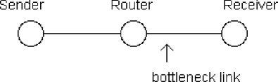
Figure 1: Network configuration

II THE MODELS

The primary mechanism used by TCP to regulate the flow of data is the congestion window on the sender’s computer. A window size of $W$ means that the number of unacknowledged packets from the sender that may be outstanding on the network at any one time is at most $W$. According to TCP, the sender’s window size follows the additive-increase/multiplicative-decrease (AIMD) scheme. Typically, the window size $W$ increases additively by $1/W$ with each successful packet transmission and decreases multiplicatively by a factor of $2$ when packets are dropped.

Packets needing to be stored in a router’s buffer due to congestion are placed in a queue. The RED module operating at this router keeps track of the queue length as well as of an exponentially-weighted average of the queue length, which we denote by $x$. When $x$ exceeds a pre-defined minimum threshold, RED will cause the router to drop arriving packets with probability that increases with $x$. Note that this adds a stochastic element to the connection. We attempt to capture the system behavior with a deterministic model; our model will not reflect the random component of the dynamics. However, as we will show below, the random component is reasonably small, and so a purely deterministic model can be useful for state estimation.

Previous attempts to model this scenario deterministically have made use of either discrete-time maps [5, 6] or differential equations [4]. Continuous-time models employing delay differential equations may do well in capturing the aspects of network behavior that evolve on small-time scales, such as flow rate increases. However, they are likely to smooth out the effects of sudden large changes in state (such as flow rate reductions). Furthermore, systems of delay differential equations can be cumbersome to express and solve due to the delay.

We address the above issues through innovations in our models, namely, a discrete impulse in the continuous-time model, the choice of time-step in the discrete-time model, and a packet-based frame of reference used by both models. The continuous-time model presented in this work combines a system of differential equations to capture the evolution of the small-time scale changes with a discrete impulse (sudden change in one of the state variables) to represent sudden large changes. The discrete-time model takes advantage of the fact that a congested bottleneck will impose uniform packet spacing. Using this spacing as the time step allows the discrete-time model to nicely capture the system behavior. In addition, as explained below, both models utilize a packet-based frame of reference for the state, which simplifies handling of the delay in the system, making the models easier to express and execute.

To describe the system, we consider the state variables, all of which have units of “packets” but are allowed to take non-integer values:

• $W$ – the congestion window size of the sender;

• $q$ – the length of the queue at the router;

• $x$ – the exponentially-weighted average of the queue length at the router.

In our packet-based frame of reference, $W(t)$ represents the congestion window in effect for a packet arriving at the queue at time $t$. This was the sender’s congestion window at an earlier time, when the packet left the sender.

In developing the models we will often refer to the round-trip time, $R$. The round-trip time is the time between the departure of a packet from the sender and the return to the sender of the acknowledgment for that packet. It consists of a fixed propagation delay, $a$, and a queuing delay. For a packet encountering a single congested router with queue length $q$, and outgoing link capacity $c$ (measured in packets per unit time), the queuing delay is $q/c$. Thus,

$$R(q)=a+\frac{q}{c}.$$ (1)

II-A THE CONTINUOUS-TIME MODEL

Our continuous-time model consists of two distinct parts. The first part is a system of differential equations similar to the one found in [4]. It is used to model the additive-increase of the window size, and both instantaneous and averaged queue lengths. The second part of the model is an impulse in which the window size state variables are instantaneously reset. This is used to model the multiplicative decrease in the window size caused by a dropped packet.

II-A1 MODELING THE ADDITIVE INCREASE

According to TCP, the window size, $W$, will normally increase by $1/W$ upon receipt of each acknowledgment. (We do not model the “slow start” phase in which the window size increases by one per received acknowledgment.) Since $W$ specifies the number of unacknowledged packets that can be out in the network at any one time, it follows that about W packets are sent per round-trip time, $R$. Thus, in approximately one round-trip time, $W$ acknowledgments return (assuming no lost packets), causing $W$ to increase by $1$. Although network data is transmitted in discrete packets, during the period of additive-increase and in the absence of dropped packets, quantities appear to vary smoothly when viewed over the time-scales we are interested in (on the order of $1$ to $100$ seconds) for our network settings. Hence we model the additive-increase of the window size continuously:

$$\frac{dW(t)}{dt}=\frac{1}{R(q(t))}.$$ (2)

The rate of change of the queue length at a given time is equal to the difference between the flows into and out of the router. By the explanation above, the flow into the router at time $t$ is $W(t)/R(q(t))$. If the queue is occupied, the flow rate out will be equal to the capacity of the router’s outgoing link, $c$. Otherwise the flow out is equal to the minimum of $c$ and the incoming flow rate.

$$\frac{dq(t)}{dt}=\left\{\begin{array}[]{ll}\frac{W(t)}{R(q(t))}-c&\mbox{when $q(t)>0$},\\ max\left(\frac{W(t)}{R(q(t))}-c,0\right)&\mbox{when $q(t)=0$}.\end{array}\right.$$ (3)

The exponentially-weighted average queue is determined by RED upon each packet arrival as follows:

$$x_{n+1}=wq_{n+1}+(1-w)x_{n},$$ (4)

where $w$ is the exponential-weighting parameter, $0\leq w\leq 1$, and the subscripts denote successive measurements of $q$ and $x$ (which occur at packet arrivals) for a given router. This equation describes a low-pass filter, and, making use of the fact that $w$ is small in practice, it can be approximated by the differential equation:

$$dx(t)/dt=w(q(t)-x(t))(W(t)/R(q(t))).$$ (5)

The term $W(t)/R(q(t))$ expresses the rate of packets arriving at the queue. The model is summarized by equations  (2), (3), and (5).

Because of our bulk-transfer and bottleneck assumptions (see Sec. I), the network is often congested to the point of saturation. This allows us to simplify the model by discarding the $q=0$ case in equation (3), and replacing the packet rate term in equation (5) with the bottleneck link capacity, $c$, as follows:

$$\frac{dW(t)}{dt}=\frac{1}{R(q(t))}$$ (6)

$$\frac{dq(t)}{dt}=\frac{W(t)}{R(q(t))}-c$$ (7)

$$\frac{dx(t)}{dt}=wc(q(t)-x(t)).$$ (8)

II-A2 MODELING THE MULTIPLICATIVE DECREASE

In a real network situation, a router using RED will drop an arriving packet with probability $p$ given by:

$$p(x)=\left\{\begin{array}[]{lll}0&\mbox{when $x<q_{min}$},\\ \frac{x-q_{min}}{q_{max}-q_{min}}p_{max}&\mbox{when $q_{min}\leq x\leq q_{max}$ },\\ 1&\mbox{when $x>q_{max}$}.\end{array}\right.$$ (9)

In practice, this usually causes a packet to be dropped soon after $x$ exceeds $q_{min}$. For the purposes of keeping our model simple and deterministic, we assume a drop occurs as soon as $x$ exceeds $q_{min}$. We continue to evolve the continuous system for one round-trip time to reflect the delay in notification of the sender that a packet has been dropped. Then we cut the window state variable, $W$, in half. Next the continuous evolution resumes but we hold the window state variable constant for one round-trip time. This is done in order to represent the Fast Recovery/Fast Retransmit(FRFR) algorithm in the NewReno version of TCP. Once this round-trip time has elapsed, the model resumes continuous evolution as described in Section  II-A1.

Denoting the continuous-time system of equations  (6), (7), and (8) by A, we can summarize the continuous-time model in hybrid systems form as in Fig. 2, where $T$ is a timer variable. The use of a hybrid system to express the model was suggested by [10]. Our model begins in the congestion avoidance phase, following the set of equations, A. Once $x$ exceeds $q_{min}$, the model assumes a drop occurs, and it transitions to the delayed drop notification phase. In this phase, it continues following the original set of equations but now it also utilizes a count-down timer, $T$, which expires one round-trip time from the time $x$ exceeds $q_{min}$. Once this timer expires, the model transitions into the recovery phase, first cutting $W$ in half and initializing a new count-down timer at the value of the present round-trip time. In the recovery phase, the equations still hold, but with one exception: $W$ is now held fixed. Finally, when this count-down timer expires, the model returns to the congestion avoidance phase.

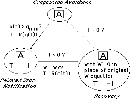
Figure 2: Hybrid systems view of the continuous-time model. A stands for equations (6), (7), and (8). $T^{\prime}=dT/dt$ and $W^{\prime}=dW/dt$.

II-A3 MODELING MULTIPLE SENDERS

The continuous-time model can be easily generalized to handle more than one sender. As in the case of one sender, we assume each additional sender is upstream from the bottleneck link and engaged in bulk transfer, sending data as fast as allowed by TCP. Following [4], denote the window size of the $i^{th}$ sender by $W_{i}$. We keep track of each sender’s window separately. The queue equation (3) is replaced by:

$$\frac{dq(t)}{dt}=\left\{\begin{array}[]{ll}(\sum_{i=1}^{N}\frac{W_{i}(t)}{R_{i}(q(t))})-c&\mbox{when $q(t)>0$},\\ max((\sum_{i=1}^{N}\frac{W_{i}(t)}{R_{i}(q(t))})-c,0)&\mbox{when $q(t)=0$}.\end{array}\right.$$ (10)

The connections need not all share the same fixed propagation delay, as the $R_{i}$ terms indicate. We use a separate copy of (2) for each window $W_{i}$, and a separate timer variable for each connection.

II-B TOWARDS A DISCRETE-TIME MODEL

In practice, the differential equations in the continuous-time model can be solved by numerical integration using a simple scheme such as Euler’s method. The main requirement is that the time step be small enough to reflect system behavior occurring on the smallest time-scale. In the given network scenario, the smallest time scale is the spacing between packets, which, as dictated by the bottleneck link, is equal to $1/c$. We will now show that the use of $1/c$ as a time step allows us to express the model in a simplified way as a discrete-time system.

The Euler numerical integration step for the $W$ equation (2), is

$$W_{k+1}=W_{k}+h\frac{1}{a+q_{k}/c},$$ (11)

where $h$ represents the time step. Setting $h=1/c$, we have

$$W_{k+1}=W_{k}+\frac{1}{ac+q_{k}}.$$ (12)

For the $q$ equation (3), neglecting the $q(t)=0$ term for the moment, the Euler step is

$$q_{k+1}=q_{k}+h\left(\frac{W_{k}}{a+q_{k}/c}-c\right),$$ (13)

which simplifies to

$$q_{k+1}=q_{k}+\frac{W_{k}}{ac+q_{k}}-1,$$ (14)

using the time step $1/c$. Note that in the above equation, the middle term represents the flow in per time step and the final term, the $-1$, represents the flow out per time step. In case the queue is empty, we omit the $-1$ term as no packets will leave within that time step:

$$q_{k+1}=\left\{\begin{array}[]{ll}q_{k}+\frac{W_{k}}{ac+q_{k}}-1&\mbox{when $q_{k}>0$},\\ q_{k}+\frac{W_{k}}{ac+q_{k}}=\frac{W_{k}}{ac}&\mbox{when $q_{k}=0$}.\end{array}\right.$$ (15)

Finally, it is easy to show that this choice of time step returns the equation for $x$ back to its original form.

$$x_{k+1}=wq_{k+1}+(1-w)x_{k}.$$ (16)

Note, we are still using the assumption that RED is updating the average queue size as if packets were arriving at the queue at a rate of $c$.

Summarizing these equations, we have a discrete-time model representation of the original continuous-time system that gives an intuitive description of the TCP dynamics on the shortest time-scale. We can utilize the same overall procedure as the continuous-time model (see Fig. 2), substituting the maps (12), (15) and (16) above for the differential equations (6), (7) and (8).

II-C THE DISCRETE-TIME MODEL

We can derive a similar but even more simplified discrete-time model by making the assumption that the system is saturated. As with the continuous-time model, the discrete-time model uses the three state variables $W$, $q$, and $x$ and consists of two primary components. The first component is a discrete-time map used to model the change in each of the state variables during the additive increase phase. The second part is an impulse that works similar to the one in the continuous-time model – it accounts for the sudden adjustment in the window size due to a dropped packet.

II-C1 MODELING THE ADDITIVE INCREASE

In practice, after an initial transient, the bottleneck link in the scenario we model will reach saturation and a queue will form at the router. Packets leave the queue at evenly spaced intervals of length $\delta=1/c$, where $c$ is the capacity of the outgoing link. For instance, if the link has a capacity of $200$ packets per second, the outgoing packets will be spaced (front-to-front) by $1/200s$ or $.005s.$ When these packets reach their destination, acknowledgment packets are sent out, with the same spacing. The arrival of the acknowledgment packets at the sender results in the sending of new data packets. Receipt of an acknowledgment frees one packet position in the TCP send window, $W$, and causes $W$ to increase by $1/W$. Typically this means that one packet is sent for each arriving acknowledgment. Occasionally, when $W$ reaches the next integer value, two packets are sent upon receipt of an acknowledgment. In other words, usually one packet arrives at the queue every $\delta$ seconds while one packet leaves the queue every $\delta$ seconds, resulting in no net change in queue length. But occasionally, $2$ packets arrive at the queue in a $\delta$-second interval while still only one leaves. This is the primary cause of queue length increase in this scenario.

The description above refers to what is sometimes known as the self-clocking nature of TCP. That is, a TCP sender has the ability to determine the limiting capacity in its flow path and send its packets at that rate. We take advantage of this behavior in our model, by employing $\delta$ as the time step in a discrete-time model of this system.

The time step is given by:

$$t_{k}=t_{0}+k\delta,\;k=0,1,2,\ldots$$ (17)

where the time $t_{0}$ marks the start of saturation. Our equation for $W$ follows directly from the rules of TCP:

$$W_{k+1}=W_{k}+\frac{1}{W_{k}}.$$ (18)

We express the change in the queue length as follows:

$$q_{k+1}=q_{k}+\frac{1}{W_{k}}.$$ (19)

While this yields fractional-valued queues, it does result in the queue length increasing by $1$ each time $W$ increases by $1$, as described above, and is simpler to express than the more realistic alternative. The equation for $x$ is the actual equation used by RED (the assumption of saturation means packets arrive each time step and so $x$ is updated each time step):

$$x_{k+1}=wq_{k}+(1-w)x_{k}.$$ (20)

The round-trip time, from (1), is:

$$R(q_{k})=a+\frac{q_{k}}{c}=\left(\frac{a}{\delta}+q_{k}\right)\delta.$$ (21)

In multiples of the time step $\delta$, the round-trip time is thus best approximated by $m_{k}=nint(a/\delta+q_{k})$ where “nint” means the nearest integer.

We initialize the additive-increase phase of the model at the start of saturation, or, in other words, at the onset of queuing. Just prior to this time, there is an exact balance between the flow in and out of the router. The flow in is equal to $W(t_{0})/R(q(t_{0}))=W(t_{0})/(a+q(t_{0})/c)$. Since $q(t_{0})=0$ at this point, the flow in is $W(t_{0})/a$ and the flow out is $c$. Thus the initial conditions for the discrete-time model are $q_{0}=0$ and $W_{0}=ca$. (Note that $W_{0}$ corresponds to the so-called bandwidth-delay product which is often used to estimate buffering for network resources.)

II-C2 MODELING THE MULTIPLICATIVE DECREASE

We model the multiplicative decrease here in much the same way as in the continuous-time model but with one additional element. As in the continuous-time model, we assume a drop occurs as soon as $x$ exceeds $q_{min}$: If $x_{k}>q_{min}$ then at time $k+m_{k}-1$, replace (18) with

$$W_{k+m_{k}}=\frac{1}{2}W_{k+m_{k}-1},$$ (22)

which reflects the delay of $1$ round-trip time in drop notification. We take advantage of the packet-level timing of this model to incorporate an additional aspect of what occurs to a network sender following a window cut. In a network, after cutting its window from $W$ to $W/2$, the sender will not send packets for $W/2$ time steps. This reflects the fact that acknowledgments for packets in the half of the window that is no longer accessible will not trigger the transmission of any new packets. As a result, the queue length will decrease. We model this by using the following equations for the next $W/2$ timesteps where $W$ is the window size just prior to the window cut:

$$W_{k+1}=W_{k},$$ (23)

$$q_{k+1}=q_{k}-1.$$ (24)

Note that $W_{k}$ remains fixed following the rules of Fast Recovery/Fast Retransmit, as was done in the continuous-time model. Next we continue to hold $W_{k}$ constant and now also hold $q_{k}$ constant to reflect the rest of the recovery period. In other words, the sender is sending packets but not increasing its window, hence the queue length should remain fixed:

$$q_{k+1}=q_{k}.$$ (25)

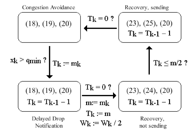
Figure 3: Hybrid systems view of the discrete-time model.

As with the continuous-time model, we can present the discrete-time model in hybrid systems form as pictured in Fig. 3. Each rounded rectangle contains the numbers of the equations to be used, and a timer variable, $T_{k}$, is utilized. The model begins in the congestion avoidance phase, obeying equations (18) , (19), and (20). Once $x$ exceeds $q_{min}$, the model assumes a drop occurs, and it transitions to the delayed drop notification phase. In this phase, it continues to obey the original set of equations, but now it also utilizes the count-down timer, $T_{k}$, which expires one round-trip time from the time $x$ exceeds $q_{min}$. (The round-trip time is given by $m_{k}$, which was defined following equation (21).) Once this timer expires, the model cuts $W_{k}$ in half, initializes a new count-down timer at the value of the present round-trip time (which we label $m$) and transitions into the recovery phase in which no packets are being sent. In this phase of the recovery, replace equations (18) and (19) used in the earlier phases, with (23) and (24), respectively. As mentioned above, this phase should last $W/2$ time steps. It is not difficult to show that this $W/2$ is equal to $.5m$ though we leave this result out for the sake of brevity. When the timer has been reduced by $.5m$, the model moves into the final state – recovery with transmission. Here it uses equations (23), (25) and (20). Finally, when the count-down timer expires, the model returns to the congestion avoidance phase.

II-C3 MODELING MULTIPLE SENDERS

In order to account for multiple senders, we must modify the discrete-time model. Consider the case of two senders, with window sizes of $W^{(1)}$ and $W^{(2)}$. Typically the senders will alternate sending windows of packets. As a result, acknowledgments will arrive at a given sender in bunches. Thus, the $1/W_{k}$ increase per time step $\delta$ indicated in (18), will not actually occur each time step for each sender. However, each connection’s window will still increase by $1$ per round-trip time. One way to reflect this in the model is to choose a time step of $2\delta$, use the original $W$ equation (18) for both senders, and change the queue equation to

$$q_{k+1}=q_{k}+\frac{1}{W^{(1)}_{k}}+\frac{1}{W^{(2)}_{k}}.$$ (26)

For $n$ senders, use a time step of $n\delta$ and include the term $1/W^{(j)}_{k}$ in the queue equation for each sender $j=1,2,...,n$.

II-D RESULTS

In this section we compare results obtained from applying our models to the network set-up mentioned above with those obtained using the ns simulator on an equivalent network. We used the settings listed in Table I.

TABLE I: Parameter Settings

Variable	Description	Value
$a$	Fixed propagation delay	.01 s
$c$	Bottleneck link capacity	1.5 Mbps
$q_{min}$	RED parameter	50
$q_{max}$	RED parameter	100
$p_{max}$	RED parameter	.1
$w$	RED parameter	.003
—-	Packet size	1000 bytes

We implemented the models in MATLAB. Since we do not model the slow-start behavior of TCP, we begin the comparison after an initial transient has ended. In Fig. 4, the top plot shows a comparison of the queue length in the continuous-time model with the results from the ns network simulator. The middle plot shows the results of the discrete-time model compared to the simulator. The bottom plot compares results from the fluid model of Misra et al. [4] with the simulator [13].

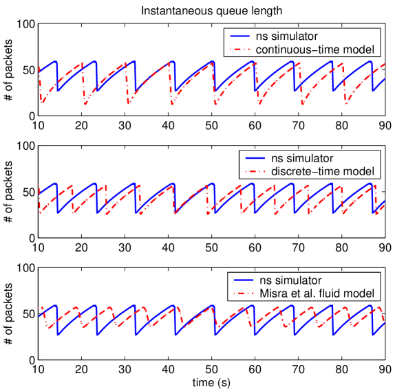
Figure 4: Comparison for one sender

Despite their lack of a stochastic component as well as several of the details of the TCP implementation, our models show good qualitative agreement with the simulator. We believe that the models have captured the essential behavior of this network under these flow conditions. The use of an impulse helps the models account for the sharp declines in the queue length caused by drop events. Lacking this feature, the fluid model of Misra et al. does not perform as well in this case of one sender.

One of the continuous-time model’s inaccuracies is that the queue length drops down too far. Lacking the no-send phase of the recovery that was included in the discrete-time model, the continuous-time model’s queue does not drop as much during the recovery period. This in turn causes $x$ to stay artificially high, high enough so that after the recovery is complete, it is still above $q_{min}$. As a result, a subsequent drop occurs, followed by an additional window cut and recovery period, all resulting in a further drop in the queue length. The consecutive recoveries’ negative contribution to queue length outweigh the positive contribution on the queue length of the lack of a no-send phase. The discrete-time model does not have this problem due to the use of the no-send recovery phase.

Another discrepancy found between our models and the simulator is in the period length of the queue oscillations. The discrete-time model’s period is too short because of the assumption of an instantaneous drop. At these settings, it takes, on average, around one second from the time RED turns on until a packet is dropped. In Sec. III we introduce a method to estimate this delay and incorporate it in the models. The continuous model’s period is too long because of the dual recovery periods which outweigh the effect just mentioned.

Fig. 5 shows a similar comparison except now we consider two senders on the network with identical fixed delays. The network has become harder to model as evidenced by the increased randomness in queue variations. Around the region $60\leq t\leq 80$, the simulator’s behavior is analogous to its typical behavior in the one-sender case. Hence, the statements made in the previous paragraph apply there. What is occurring in that region is one drop for each sender for each drop event. For much of the rest of the time interval shown, the variation is due to different drop occurrences such as two drops for one sender, only one drop, three drops and others. This suggests a modeling approach more directed towards statistical agreement than short-term qualitative agreement for cases of anything but a small number of senders.

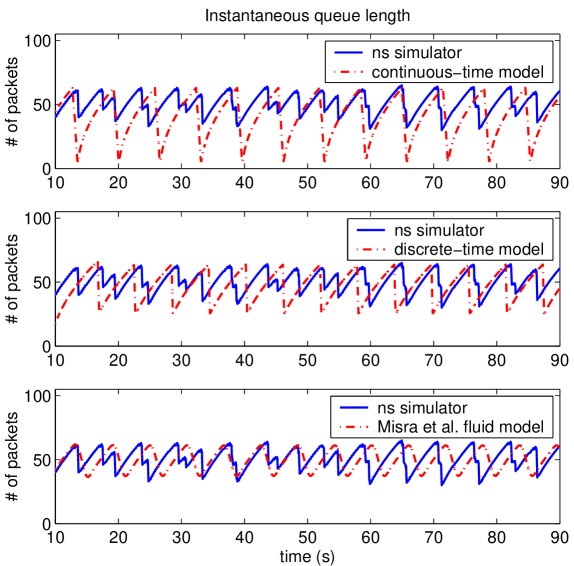
Figure 5: Comparison for two senders

For larger numbers of senders the model of Misra et al. shows better agreement with the simulator than our models do. Thus our models are advantageous mainly in cases when the bottleneck link congestion is due to a small number of senders. We propose extensions to our models in the following section to improve their performance.

III EXTENSIONS

Model simplicity is important if we are interested in being able to concisely describe a system, and for amenability to mathematical analysis. On the other hand, for the purpose of traffic state estimation, the key attributes we desire in a model are accuracy and computational efficiency. With this in mind, we introduce extensions to the models to improve their accuracy while still keeping the models simpler than a full-fledged packet-level simulator. The primary modification we consider is to implement a more realistic packet dropping mechanism within the models, one that more closely resembles RED.

III-A ESTIMATING THE INTERDROP TIME

As was mentioned in the previous section, one of the discrepancies between the models and simulator is that the models assume a drop occurs as soon as RED turns on. In reality, there tends to be a delay of about one second under the settings we are using. Here we describe a method to estimate this delay that we can incorporate into the models while still keeping them deterministic.

In practice, RED has an added layer of complexity. Namely, it has been designed so that effectively, the drop time is chosen from a uniform distribution on a time interval of length $1/p$, given a constant RED drop probability $p$. As implemented in the ns simulator [13], an additional wait parameter is used, which causes this time interval to lie between $1/p$ and $2/p$ from the time of the last drop. (This spacing also applies to the time between RED turning on and the first drop.) As a result, the expected time between drops is $3/(2p)$.

More precisely, when $x$ exceeds $q_{min}$ and RED turns on, it begins counting packets in order to determine when a packet drop should occur. The actual drop probability used by RED, which we denote $p_{drop}$, is given by:

$$p_{drop}(p,k)=\left\{\begin{array}[]{ll}0&\mbox{when $k<1/p$},\\ p/(2-kp)&\mbox{when $1/p\leq k<2/p$},\\ 1&\mbox{when $k\geq 2/p$},\end{array}\right.$$ (27)

where $k$ is the number of packets that have arrived since RED turned on, or since the previous packet drop. Let $K$ be the random variable representing the number of packets that arrive between drops, or between RED turning on and the first drop. If $x$ is constant, then $p$ is constant, in which case it can be shown that $K$ is uniformly distributed between $1/p$ and $2/p$. This means $E[K]=3/2p$.

Of course $x$ is generally not constant, and in our model we make the rough approximation that $E[K]$ is the solution to the equation $k_{drop}=3/[2p(x_{k_{drop}})]$, where $x_{k}$ is the value of $x$ when the packet counter reaches $k$. We further approximate $x$ as a linear function of $k$ between packet drops. Rewriting (4) as

$$x_{k}=x_{k-1}+w(q_{k}-x_{k-1}),$$ (28)

we replace $q_{k}-x_{k-1}$ by $q_{0}-x_{0}$:

$$x_{k}=x_{0}+kw(q_{0}-x_{0})$$ (29)

Assuming that $x_{k}$ remains between $q_{min}$ and $q_{max}$,

$$p(k)=a_{1}k+a_{2}$$ (30)

where $a_{1}$ and $a_{2}$ are constants determined by equations (9) and (29).

Since we want to find $k_{drop}$ such that $k_{drop}=3/[2p(x_{k_{drop}})]$, we substitute (30) into this equation. Solving the resulting quadratic produces the following solution:

$$k_{drop}=\frac{-a_{2}+\sqrt{a_{2}^{2}+6a_{1}}}{2a_{1}}$$ (31)

If $a_{2}^{2}+6a_{1}<0$, then since $a_{1}<0$, $p(k)$ is a decreasing function of $k$, and we assume that it becomes zero before another drop occurs.

We change the model as follows. When RED turns on, we compute $k$, the expected time until the next packet drop. A timer variable counts down this amount and when it expires, we consider the drop to have occurred and follow the same procedure as in the previous models. This scheme can be implemented for both the continuous-time and discrete-time models. In Fig. 6, we present results of its application to the continuous-time model. The figure shows that using this extension, the model is able to very closely reproduce the behavior of the simulator. However, the accuracy of this approach diminishes as the number of senders increases. For even greater accuracy, we fully implement RED as it is executed in the ns simulator. This is described in the following section.

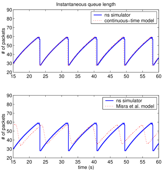
Figure 6: Comparison of models with ns simulator for the one-sender scenario described in Sec. II-D.

III-B FULL RED IMPLEMENTATION

In order to fully model RED, we begin by following the procedure laid out in the previous section up to equation (27). At that point, a uniform random number between $0$ and $1$ is generated and if this number is less than $p_{drop}$, a drop occurs. In the case of multiple senders, the probability of a given sender experiencing the drop is proportional to that sender’s share $(\frac{W_{i}}{R_{i}})/(\sum_{j=1}^{N}\frac{W_{j}}{R_{j}})$ of the overall flow. This introduces a greater degree of complexity and a stochastic component to the model. Since our ultimate goal is network traffic state estimation, our main priorities are model accuracy and computational efficiency.

We applied this model to the network described earlier, but now with four senders at varying fixed propagation delays from the receiver. Fig. 7 shows that there is good qualitative agreement between the model and the simulator. The additional jitter in the simulator’s queue is due to packet level activity. The model shows good statistical agreement with the simulator as well. Fig. 8 shows a comparison of queue histograms. Note that the model correctly captures the range in queue values, which can be used to calculate the range of round-trip times.

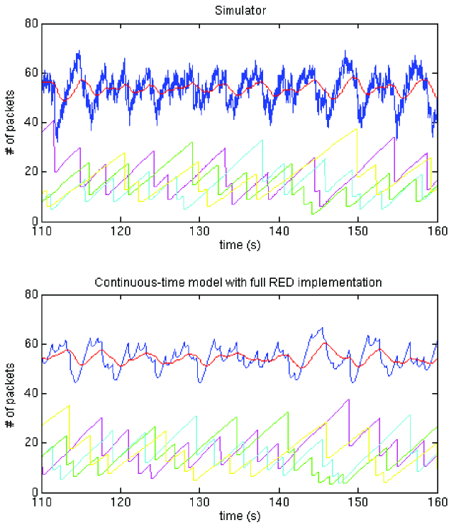
Figure 7: Comparison for four senders between the ns simulator and a realization of the continuous-time model using the full RED implementation. In both plots, the upper two curves represent the instantaneous and exponentially averaged queues. (The exponentially averaged queue is the curve showing less variation.) The lower four curves in both plots represent the window sizes of the four senders.

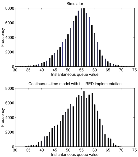
Figure 8: Comparison of instantaneous queue histograms for the four-sender network. The model is using the full RED implementation. Model queue values, which may be fractional, have been rounded for the purposes of comparison.

In order to evaluate the model’s responsiveness to network changes, we tested it on a network with two classes of flows, one of which turns off for part of the run. The classes both consist of five bulk transfer senders, but the fixed propagation delay is different for each class: $20$ ms for class $1$ senders, $35$ ms for class $2$ senders. The class $2$ senders turn off from $75$ to $125$ seconds after the start of the run. In practice, this effect could be caused by the sender-side application not having data to send for that stretch of time. Another possibility could be that the class $2$ senders are temporarily rerouted.

The results, shown in Fig. 9, indicate that the model does a good job of capturing the changes in the network state caused by the senders turning off. This includes the sudden drop in the queue just after the senders turn off. The model also reproduces the overall decreased level of the queue and increased level of the class 1 senders’ windows during the class 2 off period. Since both simulator and model have stochastic components, each plot represents a realization rather than the expected performance. Nevertheless, based on our observations of many realizations for both model and simulator, we expect the average performance to show good correspondence as well. For the time being, we give statistics from sample realizations in Table II, indicating the close statistical match between model and simulator. Note that the model is able to estimate the variance of the queue to within $10\%$. This implies that by using the model in conjunction with the round-trip time equation (1), a reasonable estimate of the variance of the round-trip time can be obtained.

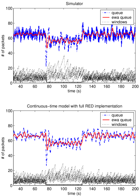
Figure 9: Comparison for two classes with five senders per class. Class 2 senders are off from 75 to 125 seconds.

TABLE II: Statistical Comparison

Variable	Quantity	Simulator	Model
All Flows On
$q$	mean	65.5	66.7
$q$	st.dev.	4.8	4.4
Half of the Flows Off
$q$	mean	56.0	56.0
$q$	st.dev.	7.0	6.5

IV TOWARDS NETWORK STATE ESTIMATION

Ultimately, we plan to use these models in a network traffic state estimation scheme. The state estimation problem can be posed as follows: Consider a network of $N$ senders and one bottleneck router, whose state can be characterized by the sender window sizes and the router queue and exponentially averaged queue lengths. Given only a series of observations of some subset of the full network state, such as the window sizes and round-trip times of a small number of senders, what is our best estimate of the state of the system at the current time? That is, we must estimate all of the sender window sizes, using only the past history of some observed portion of the state of the network.

The estimation scheme we have in mind can be described as a particle filter or, more generally, a sequential Monte Carlo method [14, 15]. The basic idea is related to that of a Kalman filter. But unlike the Kalman filter, the particle filter makes no assumptions about the linearity of the model, or about probability distributions being Gaussian. Thus it is a better fit for our model and system.

The particle filter starts off with a random ensemble of states. It uses the observation to filter and re-weight the ensemble members based on how consistent they are with the observation. Then the ensemble members are advanced in time using the model, and the filter and re-weighting process repeats. We are currently testing this procedure in a variety of network scenarios.

V CONCLUSION

We have developed two deterministic models with a discrete impulse that successfully capture the network behavior of TCP/RED in simple cases. Extending the models by adding a stochastic dropping mechanism consistent with RED, the models shows good correspondence in more complicated network situations, including those with larger numbers of senders and flows turning on and off.

Aside from network traffic state estimation described in Sec. IV, other works in progress include estimation of some dynamical properties such as period length, maximum sender window size and drop rate. Additionally, we are applying our models to networks subject to cross-traffic, including one that is prone to irregular behavior due to the presence of a source that sends large bursts of packets at regular intervals.

References

- [1] A. Medina, M. Allman and S. Floyd, “Measuring the Evolution of Transport Protocols in the Internet”, preprint, available from http://www.icir.org/tbit.
- [2] M. Fomenkov, K. Keys, D. Moore and k claffy, “Longitudinal Study of Internet Traffic in 1998-2003”, technical report, Cooperative Association for Internet Data Analysis (CAIDA), 2003.
- [3] S. Floyd and V. Jacobson, “Random Early Detection Gateways for Congestion Avoidance,” IEEE Trans. on Networking, Vol.1, no. 7, pp. 397-413, 1993.
- [4] V. Misra, W. Gong, D. Towsley. “Fluid-based Analysis of a Network of AQM Routers Supporting TCP Flows with an Application to RED,” Proc. of SIGCOMM 2000.
- [5] V. Firoiu and M. Borden, “Study of Active Queue Management for Congestion Control,” Proc. of Infocom 2000.
- [6] P. Ranjan, E. Abed and R. La, “Nonlinear Instabilities in TCP-RED,” Proc. of Infocom 2002.
- [7] S.H. Low, F. Paganini, J. Wang, S. Adlakha and J. Doyle, “Dynamics of TCP/RED and a Scalable Control,” Proc. of Infocom 2002.
- [8] M. Mathis, J. Semke, J. Mahdavi, and T. Ott, “The Macroscopic Behavior of the TCP Congestion Avoidance Algorithm,” Computer Communications Review, Vol. 27, no. 3, 1997.
- [9] J. Padhye, V. Firoiu, D. Towsley, and J. Kurose, “Modeling TCP Throughput: A Simple Model and its Empirical Validation,” Proc. of SIGCOMM 1998.
- [10] J. Hespanha, S. Bohacek, K. Obraczka and J. Lee, “Hybrid Modeling of TCP Congestion Control,” Lecture Notes in Computer Science, no. 2034, pp. 291-304, 2001.
- [11] S. Bohacek, J. Hespanha, J. Lee and K. Obraczka, “A Hybrid Systems Modeling Framework for Fast and Accurate Simulation of Data Communication Networks,” Proc. of SIGMETRICS 2003.
- [12] Y. Liu, F. Lo Presti, V. Misra, D. Towsley and Y. Gu, “Fluid Models and Solutions for Large-Scale IP Networks,” Proc. of SIGMETRICS 2003.
- [13] http://www.isi.edu/nsnam/ns/
- [14] N. Gordon, D. Salmond and A. Smith, “Novel approach to nonlinear/non-Gaussian Bayesian state estimation,” IEE Proceedings-F, Vol. 140, no. 2, pp. 107-113, 1993.
- [15] A. Doucet, N. de Freitas, N. Gordon, eds., Sequential Monte Carlo Methods in Practice, Springer, New York, 2001.