Improved Approximate String Matching and Regular Expression Matching on Ziv-Lempel Compressed Texts

Abstract

We study the approximate string matching and regular expression matching problem for the case when the text to be searched is compressed with the Ziv-Lempel adaptive dictionary compression schemes. We present a time-space trade-off that leads to algorithms improving the previously known complexities for both problems. In particular, we significantly improve the space bounds, which in practical applications are likely to be a bottleneck.

1 Introduction

Modern text databases, e.g. for biological and World Wide Web data, are huge. To save time and space, it is desireable if data can be kept in compressed form and still allow efficient searching. Motivated by this Amir and Benson [2, 3] initiated the study of compressed pattern matching problems, that is, given a text string $Q$ in compressed form $Z$ and a specified (uncompressed) pattern $P$, find all occurrences of $P$ in $Q$ without decompressing $Z$. The goal is to search more efficiently than the naïve approach of decompressing $Z$ into $Q$ and then searching for $P$ in $Q$. Various compressed pattern matching algorithms have been proposed depending on the type of pattern and compression method, see e.g., [3, 9, 12, 11, 19, 14]. For instance, given a string $Q$ of length $u$ compressed with the Ziv-Lempel-Welch scheme [24] into a string of length $n$, Amir et al. [4] gave an algorithm for finding all exact occurrences of a pattern string of length $m$ in $O(n+m^{2})$ time and space.

In this paper we study the classical approximate string matching and regular expression matching problems in the context of compressed texts. As in previous work on these problems [11, 19] we focus on the popular ZL78  and ZLW  adaptive dictionary compression schemes [26, 24]. We present a new technique that gives a general time-space trade-off. The resulting algorithms improve all previously known complexities for both problems. In particular, we significantly improve the space bounds. When searching large text databases, space is likely to be a bottleneck and therefore this is of crucial importance.

1.1 Approximate String Matching

Given strings $P$ and $Q$ and an error threshold $k$, the classical approximate string matching problem is to find all ending positions of substrings of $Q$ whose edit distance to $P$ is at most $k$. The edit distance between two strings is the minimum number of insertions, deletions, and substitutions needed to convert one string to the other. The classical dynamic programming solution due to Sellers [22] solves the problem in $O(um)$ time and $O(m)$ space, where $u$ and $m$ are the length of $Q$ and $P$, respectively. Several improvements of this result are known, see e.g., the survey by Navarro [18]. For this paper we are particularly interested in the fast solution for small values of $k$, namely, the $O(uk)$ time algorithm by Landau and Vishkin [13] and the more recent $O(uk^{4}/m+u)$ time algorithm due to Cole and Hariharan [7] (we assume w.l.o.g. that $k<m$). Both of these can be implemented in $O(m)$ space.

Recently, Kärkkäinen et al. [11] studied this problem for text compressed with the ZL78/ZLW  compression schemes. If $n$ is the length of the compressed text, their algorithm achieves $O(nmk+\mathit{occ})$ time and $O(nmk)$ space, where $\mathit{occ}$ is the number of occurrences of the pattern. Currently, this is the only non-trivial worst-case bound for the general problem on compressed texts. For special cases and restricted versions, other algorithms have been proposed [15, 21]. An experimental study of the problem and an optimized practical implementation can be found in [20].

In this paper, we show that the problem is closely connected to the uncompressed problem and we achieve a simple time-space trade-off. More precisely, let $t(m,u,k)$ and $s(m,u,k)$ denote the time and space, respectively, needed by any algorithm to solve the (uncompressed) approximate string matching problem with error threshold $k$ for pattern and text of length $m$ and $u$, respectively. We show the following result.

Theorem 1

Let $Q$ be a string compressed using ZL78 into a string $Z$ of length $n$ and let $P$ be a pattern of length $m$. Given $Z$, $P$, and a parameter $\tau\geq 1$, we can find all approximate occurrences of $P$ in $Q$ with at most $k$ errors in $O(n(\tau+m+t(m,2m+2k,k))+\mathit{occ})$ expected time and $O(n/\tau+m+s(m,2m+2k,k)+\mathit{occ})$ space.

The expectation is due to hashing and can be removed at an additional $O(n)$ space cost. In this case the bound also hold for ZLW  compressed strings. We assume that the algorithm for the uncompressed problem produces the matches in sorted order (as is the case for all algorithms that we are aware of). Otherwise, additional time for sorting must be included in the bounds. To compare Theorem 1 with the result of Karkkainen et al. [11], plug in the Landau-Vishkin algorithm and set $\tau=mk$. This gives an algorithm using $O(nmk+\mathit{occ})$ time and $O(n/mk+m+\mathit{occ})$ space. This matches the best known time bound while improving the space by a factor $\Theta(m^{2}k^{2})$. Alternatively, if we plug in the Cole-Hariharan algorithm and set $\tau=k^{4}+m$ we get an algorithm using $O(nk^{4}+nm+\mathit{occ})$ time and $O(n/(k^{4}+m)+m+\mathit{occ})$ space. Whenever $k=O(m^{1/4})$ this is $O(nm+\mathit{occ})$ time and $O(n/m+m+\mathit{occ})$ space.

To the best of our knowledge, all previous non-trivial compressed pattern matching algorithms for ZL78/ZLW  compressed text, with the exception of a very slow algorithm for exact string matching by Amir et al. [4], use $\Omega(n)$ space. This is because the algorithms explicitly construct the dictionary trie of the compressed texts. Surprisingly, our results show that for the ZL78  compression schemes this is not needed to get an efficient algorithm. Conversely, if very little space is available our trade-off shows that it is still possible to solve the problem without decompressing the text.

1.2 Regular Expression Matching

Given a regular expression $R$ and a string $Q$, the regular expression matching problem is to find all ending position of substrings in $Q$ that matches a string in the language denoted by $R$. The classic textbook solution to this problem due to Thompson [23] solves the problem in $O(um)$ time and $O(m)$ space, where $u$ and $m$ are the length of $Q$ and $R$, respectively. Improvements based on the Four Russian Technique or word-level parallelism are given in [17, 6, 5].

The only solution to the compressed problem is due to Navarro [19]. His solution depends on word RAM techniques to encode small sets into memory words, thereby allowing constant time set operations. On a unit-cost RAM with $w$-bit words this technique can be used to improve an algorithm by at most a factor $O(w)$. For $w=O(\log u)$ a similar improvement is straightforward to obtain for our algorithm and we will therefore, for the sake of exposition, ignore this factor in the bounds presented below. With this simplification Navarro’s algorithm uses $O(nm^{2}+\mathit{occ}\cdot m\log m)$ time and $O(nm^{2})$ space, where $n$ is the length of the compressed string. In this paper we show the following time-space trade-off:

Theorem 2

Let $Q$ be a string compressed using ZL78 or ZLW into a string $Z$ of length $n$ and let $R$ be a regular expression of length $m$. Given $Z$, $R$, and a parameter $\tau\geq 1$, we can find all occurrences of substrings matching $R$ in $Q$ in $O(nm(m+\tau)+\mathit{occ}\cdot m\log m)$ time and $O(nm^{2}/\tau+nm)$ space.

If we choose $\tau=m$ we obtain an algorithm using $O(nm^{2}+\mathit{occ}\cdot m\log m)$ time and $O(nm)$ space. This matches the best known time bound while improving the space by a factor $\Theta(m)$. With word-parallel techniques these bounds can be improved slightly. The full details are given in Section 4.5.

1.3 Techniques

If pattern matching algorithms for ZL78 or ZLW compressed texts use $\Omega(n)$ working space they can explicitly store the dictionary trie for the compressed text and apply any linear space data structure to it. This has proven to be very useful for compressed pattern matching. However, as noted by Amir et al. [4], $\Omega(n)$ working space may not be feasible for large texts and therefore more space-efficient algorithms are needed. Our main technical contribution is a simple $o(n)$ data structure for ZL78 compressed texts. The data structure gives a way to compactly represent a subset of the trie which combined with the compressed text enables algorithms to quickly access relevant parts of the trie. This provides a general approach to solve compressed pattern matching problems in $o(n)$ space, which combined with several other techniques leads to the above results.

2 The Ziv-Lempel Compression Schemes

Let $\Sigma$ be an alphabet containing $\sigma=|\Sigma|$ characters. A string $Q$ is a sequence of characters from $\Sigma$. The length of $Q$ is $u=|Q|$ and the unique string of length $0$ is denoted $\epsilon$. The $i$th character of $Q$ is denoted $Q[i]$ and the substring beginning at position $i$ of length $j-i+1$ is denoted $Q[i,j]$. The Ziv-Lempel algorithm from 1978 [26] provides a simple and natural way to represent strings, which we describe below. Define a ZL78 compressed string (abbreviated compressed string in the remainder of the paper) to be a string of the form

$$Z=z_{1}\cdots z_{n}=(r_{1},\alpha_{1})(r_{2},\alpha_{2})\ldots(r_{n},\alpha_{n}),$$

where $r_{i}\in\{0,\ldots,i-1\}$ and $\alpha_{i}\in\Sigma$. Each pair $z_{i}=(r_{i},\alpha_{i})$ is a compression element, and $r_{i}$ and $\alpha_{i}$ are the reference and label of $z_{i}$, denoted by $\mathrm{reference}(z_{i})$ and $\mathrm{label}(z_{i})$, respectively. Each compression element represents a string, called a phrase. The phrase for $z_{i}$, denoted $\mathrm{phrase}(z_{i})$, is given by the following recursion.

$$\mathrm{phrase}(z_{i})=\begin{cases}\mathrm{label}(z_{i})&\text{if $\mathrm{reference}(z_{i})=0$},\\ \mathrm{phrase}(\mathrm{reference}(z_{i}))\cdot\mathrm{label}(z_{i})&\text{otherwise}.\end{cases}$$

The $\cdot$ denotes concatenation of strings. The compressed string $Z$ represents the concatenation of the phrases, i.e., the string $\mathrm{phrase}(z_{1})\cdots\mathrm{phrase}(z_{n})$.

Let $Q$ be a string of length $u$. In ZL78, the compressed string representing $Q$ is obtained by greedily parsing $Q$ from left-to-right with the help of a dictionary $D$. For simplicity in the presentation we assume the existence of an initial compression element $z_{0}=(0,\epsilon)$ where $\mathrm{phrase}(z_{0})=\epsilon$. Initially, let $z_{0}=(0,\epsilon)$ and let $D=\{\epsilon\}$. After step $i$ we have computed a compressed string $z_{0}z_{1}\cdots z_{i}$ representing $Q[1,j]$ and $D=\{\mathrm{phrase}(z_{0}),\ldots,\mathrm{phrase}(z_{i})\}$. We then find the longest prefix of $Q[j+1,u-1]$ that matches a string in $D$, say $\mathrm{phrase}(z_{k})$, and let $\mathrm{phrase}(z_{i+1})=\mathrm{phrase}(z_{k})\cdot Q[j+1+|\mathrm{phrase}(z_{k})|]$. Set $D=D\cup\{\mathrm{phrase}(z_{i+1})\}$ and let $z_{i+1}=(k,Q[j+1+|\mathrm{phrase}(z_{i+1})|])$. The compressed string $z_{0}z_{1}\ldots z_{i+1}$ now represents the string $Q[1,j+|\mathrm{phrase}(z_{i+1})|])$ and $D=\{\mathrm{phrase}(z_{0}),\ldots,\mathrm{phrase}(z_{i+1})\}$. We repeat this process until all of $Q$ has been read.

Since each phrase is the concatenation of a previous phrase and a single character, the dictionary $D$ is prefix-closed, i.e., any prefix of a phrase is a also a phrase. Hence, we can represent it compactly as a trie where each node $i$ corresponds to a compression element $z_{i}$ and $\mathrm{phrase}(z_{i})$ is the concatenation of the labels on the path from $z_{i}$ to node $i$. Due to greediness, the phrases are unique and therefore the number of nodes in $D$ for a compressed string $Z$ of length $n$ is $n+1$. An example of a string and the corresponding compressed string is given in Fig. 1.

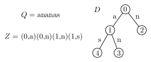
Figure 1: The compressed string $Z$ representing $Q$ and the corresponding dictionary trie $D$. Taken from [19].

Throughout the paper we will identify compression elements with nodes in the trie $D$, and therefore we use standard tree terminology, briefly summed up here: The distance between two elements is the number of edges on the unique simple path between them. The depth of element $z$ is the distance from $z$ to $z_{0}$ (the root of the trie). An element $x$ is an ancestor of an element $z$ if $\mathrm{phrase}(x)$ is a prefix of $\mathrm{phrase}(z)$. If also $|\mathrm{phrase}(x)|=|\mathrm{phrase}(z)|-1$ then $x$ is the parent of $z$. If $x$ is ancestor of $z$ then $z$ is a descendant of $x$ and if $x$ is the parent of $z$ then $z$ is the child of $x$.The length of a path $p$ is the number of edges on the path, and is denoted $|p|$. The label of a path is the concatenation of the labels on these edges.

Note that for a compression element $z$, $\mathrm{reference}(z)$ is a pointer to the parent of $z$ and $\mathrm{label}(z)$ is the label of the edge to the parent of $z$. Thus, given $z$ we can use the compressed text $Z$ directly to decode the label of the path from $z$ towards the root in constant time per element. We will use this important property in many of our results.

If the dictionary $D$ is implemented as a trie it is straightforward to compress $Q$ or decompress $Z$ in $O(u)$ time. Furthermore, if we do not want to explicitly decompress $Z$ we can compute the trie in $O(n)$ time, and as mentioned above, this is done in almost all previous compressed pattern matching algorithm on Ziv-Lempel compression schemes. However, this requires at least $\Omega(n)$ space which is insufficient to achieve our bounds. In the next section we show how to partially represent the trie in less space.

2.1 Selecting Compression Elements

Let $Z=z_{0}\ldots z_{n}$ be a compressed string. For our results we need an algorithm to select a compact subset of the compression elements such that the distance from any element to an element in the subset is no larger than a given threshold. More precisely, we show the following lemma.

Lemma 1

Let $Z$ be a compressed string of length $n$ and let $1\leq\tau\leq n$ be parameter. There is a set of compression elements $C$ of $Z$, computable in $O(n\tau)$ expected time and $O(n/\tau)$ space with the following properties:

• $|C|=O(n/\tau)$.

• For any compression element $z_{i}$ in $Z$, the minimum distance to any compression element in $C$ is at most $2\tau$.

Proof. Let $1\leq\tau\leq n$ be a given parameter. We build $C$ incrementally in a left-to-right scan of $Z$. The set is maintained as a dynamic dictionary using dynamic perfect hashing [8], i.e., constant time worst-case access and constant time amortized expected update. Initially, we set $C=\{z_{0}\}$. Suppose that we have read $z_{0},\ldots,z_{i}$. To process $z_{i+1}$ we follow the path $p$ of references until we encounter an element $y$ such that $y\in C$. We call $y$ the nearest special element of $z_{i+1}$. Let $l$ be the number of elements in $p$ including $z_{i+1}$ and $y$. Since each lookup in $C$ takes constant time the time to find the nearest special element is $O(l)$. If $l<2\cdot\tau$ we are done. Otherwise, if $l=2\cdot\tau$, we find the $\tau$th element $y^{\prime}$ in the reference path and set $C:=C\cup\{y^{\prime}\}$. As the trie grows under addition of leaves condition (ii) follows. Moreover, any element chosen to be in $C$ has at least $\tau$ descendants of distance at most $\tau$ that are not in $C$ and therefore condition (i) follows. The time for each step is $O(\tau)$ amortized expected and therefore the total time is $O(n\tau)$ expected. The space is proportional to the size of $C$ hence the result follows. $\Box$

2.2 Other Ziv-Lempel Compression Schemes

A popular variant of ZL78  is the ZLW compression scheme [24]. Here, the label of compression elements are not explicitly encoded, but are defined to be the first character of the next phrase. Hence, ZLW does not offer an asymptotically better compression ratio over ZL78 but gives a better practical performance. The ZLW scheme is implemented in the UNIX program compress. From an algorithmic viewpoint ZLW is more difficult to handle in a space-efficient manner since labels are not explicitly stored with the compression elements as in ZL78. However, if $\Omega(n)$ space is available then we can simply construct the dictionary trie. This gives constant time access to the label of a compression elements and therefore ZL78 and ZLW become ”equivalent”. This is the reason why Theorem 1 holds only for ZL78 when space is $o(n)$ but for both when the space is $\Omega(n)$.

Another well-known variant is the ZL77 compression scheme [25]. Unlike ZL78 and ZLW phrases in the ZL77 scheme can be any substring of text that has already been processed. This makes searching much more difficult and none of the known techniques for ZL78 and ZLW seems to be applicable. The only known algorithm for pattern matching on ZL77 compressed text is due to Farach and Thorup [9] who gave an algorithm for the exact string matching problem.

3 Approximate String Matching

In this section we consider the compressed approximate string matching problem. Before presenting our algorithm we need a few definitions and properties of approximate string matching.

Let $A$ and $B$ be strings. Define the edit distance between $A$ and $B$, $\gamma(A,B)$, to be the minimum number of insertions, deletions, and substitutions needed to transform $A$ to $B$. We say that $j\in[1,|S|]$ is a match with error at most $k$ of $A$ in a string $S$ if there is an $i\in[1,j]$ such that $\gamma(A,S[i,j])\leq k$. Whenever $k$ is clear from the context we simply call $j$ a match. All positions $i$ satisfying the above property are called a start of the match $j$. The set of all matches of $A$ in $S$ is denoted $\Gamma(A,S)$. We need the following well-known property of approximate matches.

Proposition 1

Any match $j$ of $A$ in $S$ with at most $k$ errors must start in the interval $[\max(1,j-|A|+1-k),\min(|S|,j-|A|+1+k)]$.

Proof. Let $l$ be the length of a substring $B$ matching $A$ and ending at $j$. If the match starts outside the interval then either $l<|A|-k$ or $l>|A|+k$. In these cases, more than $k$ deletions or $k$ insertions, respectively, are needed to transform $B$ to $A$. $\Box$

3.1 Searching for Matches

Let $P$ be a string of length $m$ and let $k$ be an error threshold. To avoid trivial cases we assume that $k<m$. Given a compressed string $Z=z_{0}z_{1}\ldots z_{n}$ representing a string $Q$ of length $u$ we show how to find $\Gamma(P,Q)$ efficiently.

Let $l_{i}=|\mathrm{phrase}(z_{i})|$, let $u_{0}=1$, and let $u_{i}=u_{i-1}+l_{i-1}$, for $1\leq i\leq n$, i.e., $l_{i}$ is the length of the $i$th phrase and $u_{i}$ is the starting position in $Q$ of the $i$th phrase. We process $Z$ from left-to-right and at the $i$th step we find all matches in $[u_{i},u_{i}+l_{i}-1]$. Matches in this interval can be either internal or overlapping (or both). A match $j$ in $[u_{i},u_{i}+l_{i}-1]$ is internal if it has a starting point in $[u_{i},u_{i}+l_{i}-1]$ and overlapping if it has a starting point in $[1,u_{i}-1]$. To find all matches we will compute the following information for $z_{i}$.

• The start position, $u_{i}$, and length, $l_{i}$, of $\mathrm{phrase}(z_{i})$.

• The relevant prefix, $\mathrm{rpre}(z_{i})$, and the relevant suffix, $\mathrm{rsuf}(z_{i})$, where

  $$\mathrm{rpre}(z_{i}) =Q[u_{i},\min(u_{i}+m+k-1,u_{i}+l_{i}-1)]\;,$$

  $$\mathrm{rsuf}(z_{i}) =Q[\max(1,u_{i}+l_{i}-m-k),u_{i}+l_{i}-1]\;.$$

  In other words, $\mathrm{rpre}(z_{i})$ is the largest prefix of length at most $m+k$ of $\mathrm{phrase}(z_{i})$ and $\mathrm{rsuf}(z_{i})$ is the substring of length $m+k$ ending at $u_{i}+l_{i}-1$. For an example see Fig. 2.

• The match sets $M_{I}(z_{i})$ and $M_{O}(z_{i})$, where

  $$M_{I}(z_{i}) =\Gamma(P,\mathrm{phrase}(z_{i}))\;,$$

  $$M_{O}(z_{i}) =\Gamma(P,\mathrm{rsuf}(z_{i-1})\cdot\mathrm{rpre}(z_{i}))\;.$$

  We assume that both sets are represented as sorted lists in increasing order.

Figure 2: The relevant prefix and the relevant suffix of two phrases in $Q$. Here, $|\mathrm{phrase}(z_{i-1})|<m+k$ and therefore $\mathrm{rsuf}(z_{i-1})$ overlaps with previous phrases.

We call the above information the description of $z_{i}$. In the next section we show how to efficiently compute descriptions. For now, assume that we are given the description of $z_{i}$. Then, the set of matches in $[u_{i},u_{i}+l_{i}-1]$ is reported as the set

$$M(z_{i}) = \{j+u_{i}-1\mid j\in M_{I}(z_{i})\}\cup$$

$$\{j+u_{i}-1-|\mathrm{rsuf}(z_{i-1})|\mid j\in M_{O}(z_{i})\cap[u_{i},u_{i}+l_{i}-1]\}\;.$$

We argue that this is the correct set. Since $\mathrm{phrase}(z_{i})=Q[u_{i},u_{i}+l_{i}-1]$ we have that

$$j\in M_{I}(z_{i})\Leftrightarrow j+u_{i}-1\in\Gamma(P,Q[u_{i},u_{i}+l_{i}-1]\;.$$

Hence, the set $\{j+u_{i}-1\mid j\in M_{I}(z_{i})\}$ is the set of all internal matches. Similarly, $\mathrm{rsuf}(z_{i-1})\cdot\mathrm{rpre}(z_{i})=Q[u_{i}-|\mathrm{rsuf}(z_{i-1})|,u_{i}+|\mathrm{rpre}(z_{i})|-1]$ and therefore

$$j\in M_{O}(z_{i})\Leftrightarrow j+u_{i}-1-|\mathrm{rsuf}(z_{i-1})|\in\Gamma(P,Q[u_{i}-|\mathrm{rsuf}(z_{i-1})|,u_{i}+1+|\mathrm{rpre}(z_{i})|])\;.$$

By Proposition 1 any overlapping match must start at a position within the interval $[\max(1,u_{i}-m+1-k),u_{i}]$. Hence, $\{j+u_{i}-1-|\mathrm{rsuf}(z_{i-1})|\mid j\in M_{O}(z_{i})\}$ includes all overlapping matches in $[u_{i},u_{i}+l_{i}-1]$. Taking the intersection with $[u_{i},u_{i}+l_{i}-1]$ and the union with the internal matches it follows that the set $M(z_{i})$ is precisely the set of matches in $[u_{i},u_{i}+l_{i}-1]$. For an example see Fig. 3.

$$Q=\textrm{ananasbananer},\quad P=\textrm{base},\quad Z=\textrm{(0,a)(0,n)(1,n)(1,s)(0,b)(3,a)(2,e)(0,r)}$$

Descriptions

$\begin{array}[]{l @{\hspace{5pt}} | @{\hspace{5pt}} l @{\hspace{5pt}} l @{\hspace{5pt}} l @{\hspace{5pt}} l @{\hspace{5pt}} l @{\hspace{5pt}} l @{\hspace{5pt}} l @{\hspace{5pt}} l}\hline\cr\hfil\hskip 5.0pt\vrule\hskip 5.0&z_{0}\hfil\hskip 5.0&z_{1}\hfil\hskip 5.0&z_{2}\hfil\hskip 5.0&z_{3}\hfil\hskip 5.0&z_{4}\hfil\hskip 5.0&z_{5}\hfil\hskip 5.0&z_{6}\hfil\hskip 5.0&z_{7}\\ \hline\cr u_{i}\hfil\hskip 5.0pt\vrule\hskip 5.0&1\hfil\hskip 5.0&2\hfil\hskip 5.0&3\hfil\hskip 5.0&5\hfil\hskip 5.0&7\hfil\hskip 5.0&8\hfil\hskip 5.0&11\hfil\hskip 5.0&13\\ l_{i}\hfil\hskip 5.0pt\vrule\hskip 5.0&1\hfil\hskip 5.0&1\hfil\hskip 5.0&2\hfil\hskip 5.0&2\hfil\hskip 5.0&1\hfil\hskip 5.0&3\hfil\hskip 5.0&2\hfil\hskip 5.0&1\\ \textrm{rpre}(z_{i})\hfil\hskip 5.0pt\vrule\hskip 5.0&\textrm{a}\hfil\hskip 5.0&\textrm{n}\hfil\hskip 5.0&\textrm{an}\hfil\hskip 5.0&\textrm{as}\hfil\hskip 5.0&\textrm{b}\hfil\hskip 5.0&\textrm{ana}\hfil\hskip 5.0&\textrm{ne}\hfil\hskip 5.0&\textrm{r}\\ \textrm{rsuf}(z_{i})\hfil\hskip 5.0pt\vrule\hskip 5.0&\textrm{a}\hfil\hskip 5.0&\textrm{an}\hfil\hskip 5.0&\textrm{anas}\hfil\hskip 5.0&\textrm{ananas}\hfil\hskip 5.0&\textrm{nanasb}\hfil\hskip 5.0&\textrm{asbana}\hfil\hskip 5.0&\textrm{banane}\hfil\hskip 5.0&\textrm{ananer}\\ M_{I}(z_{i})\hfil\hskip 5.0pt\vrule\hskip 5.0&\emptyset\hfil\hskip 5.0&\emptyset\hfil\hskip 5.0&\emptyset\hfil\hskip 5.0&\{2\}\hfil\hskip 5.0&\emptyset\hfil\hskip 5.0&\emptyset\hfil\hskip 5.0&\emptyset\hfil\hskip 5.0&\emptyset\\ M_{O}(z_{i})\hfil\hskip 5.0pt\vrule\hskip 5.0&\emptyset\hfil\hskip 5.0&\emptyset\hfil\hskip 5.0&\emptyset\hfil\hskip 5.0&\{6\}\hfil\hskip 5.0&\{6,7\}\hfil\hskip 5.0&\{5,6,7,8\}\hfil\hskip 5.0&\{2,3,4,5,6\}\hfil\hskip 5.0&\{2,3,4,6\}\\ M(z_{i})\hfil\hskip 5.0pt\vrule\hskip 5.0&\emptyset\hfil\hskip 5.0&\emptyset\hfil\hskip 5.0&\emptyset\hfil\hskip 5.0&\{6\}\hfil\hskip 5.0&\{7\}\hfil\hskip 5.0&\{8,9,10\}\hfil\hskip 5.0&\{12\}\hfil\hskip 5.0&\emptyset\end{array}$

Figure 3: Example of descriptions. $Z$ is the compressed string representing $Q$. We are looking for all matches of the pattern $P$ with error threshold $k=2$ in $Z$. The set of matches is $\{6,7,8,9,10,12\}$.

Next we consider the complexity of computing the matches. To do this we first bound the size of the $M_{I}$ and $M_{O}$ sets. Since the length of any relevant suffix and relevant prefix is at most $m+k$, we have that $|M_{O}(z_{i})|\leq 2(m+k)<4m$, and therefore the total size of the $M_{O}$ sets is at most $O(nm)$. Each element in the sets $M_{I}(z_{0}),\ldots,M_{I}(z_{n})$ corresponds to a unique match. Thus, the total size of the $M_{I}$ sets is at most $\mathit{occ}$, where $\mathit{occ}$ is the total number of matches. Since both sets are represented as sorted lists the total time to compute the matches for all compression elements is $O(nm+\mathit{occ})$.

3.2 Computing Descriptions

Next we show how to efficiently compute the descriptions. Let $1\leq\tau\leq n$ be a parameter. Initially, we compute a subset $C$ of the elements in $Z$ according to Lemma 1 with parameter $\tau$. For each element $z_{j}\in C$ we store $l_{j}$, that is, the length of $\mathrm{phrase}(z_{j})$. If $l_{j}>m+k$ we also store the index of the ancestor $x$ of $z_{j}$ of depth $m+k$. This information can easily be computed while constructing $C$ within the same time and space bounds, i.e., using $O(n\tau)$ time and $O(n/\tau)$ space.

Descriptions are computed from left-to-right as follows. Initially, set $l_{0}=0$, $u_{0}=0$, $\mathrm{rpre}(z_{0})=\epsilon$, $\mathrm{rsuf}(z_{0})=\epsilon$, $M_{I}(z_{0})=\emptyset$, and $M_{O}(z_{0})=\emptyset$. To compute the description of $z_{i}$, $1\leq i\leq n$, first follow the path $p$ of references until we encounter an element $z_{j}\in C$. Using the information stored at $z_{j}$ we set $l_{i}:=|p|+l_{j}$ and $u_{i}=u_{i-1}+l_{i-1}$. By Lemma 1(ii) the distance to $z_{j}$ is at most $2\tau$ and therefore $l_{i}$ and $u_{i}$ can be computed in $O(\tau)$ time given the description of $z_{i-1}$.

To compute $\mathrm{rpre}(z_{i})$ we compute the label of the path from $z_{0}$ towards $z_{i}$ of length $\min(m+k,l_{i})$. There are two cases to consider: If $l_{i}\leq m+k$ we simply compute the label of the path from $z_{i}$ to $z_{0}$ and let $\mathrm{rpre}(z_{i})$ be the reverse of this string. Otherwise ($l_{i}>m+k$), we use the ”shortcut” stored at $z_{j}$ to find the ancestor $z_{h}$ of distance $m+k$ to $z_{0}$. The reverse of the label of the path from $z_{h}$ to $z_{0}$ is then $\mathrm{rpre}(z_{i})$. Hence, $\mathrm{rpre}(z_{i})$ is computed in $O(m+k+\tau)=O(m+\tau)$ time.

The string $\mathrm{rsuf}(z_{i})$ may be the divided over several phrases and we therefore recursively follow paths towards the root until we have computed the entire string. It is easy to see that the following algorithm correctly decodes the desired substring of length $\min(m+k,u_{i})$ ending at position $u_{i}+l_{i}-1$.

1. Initially, set $l:=\min(m+k,u_{i}+l_{i}-1)$, $t:=i$, and $s:=\epsilon$.

2. Compute the path $p$ of references from $z_{t}$ of length $r=\min(l,0pt(z_{t}))$ and set $s:=s\cdot\mathrm{label}(p)$.

3. If $r<l$ set $l:=l-r$, $t:=t-1$, and repeat step $2$.

4. Return $\mathrm{rsuf}(z_{i})$ as the reverse of $s$.

Since the length of $\mathrm{rsuf}(z_{i})$ is at most $m+k$, the algorithm finds it in $O(m+k)=O(m)$ time.

The match sets $M_{I}$ and $M_{O}$ are computed as follows. Let $t(m,u,k)$ and $s(m,u,k)$ denote the time and space to compute $\Gamma(A,B)$ with error threshold $k$ for strings $A$ and $B$ of lengths $m$ and $u$, respectively. Since $|\mathrm{rsuf}(z_{i-1})\cdot\mathrm{rpre}(z_{i})|\leq 2m+2k$ it follows that $M_{O}(z_{i})$ can be computed in $t(m,2m+2k,k)$ time and $s(m,2m+2k,k)$ space. Since $M_{I}(z_{i})=\Gamma(P,\mathrm{phrase}(z_{i}))$ we have that $j\in M_{I}(z_{i})$ if and only if $j\in M_{I}(\mathrm{reference}(z_{i}))$ or $j=l_{i}$. By Proposition 1 any match ending in $l_{i}$ must start within $[\max(1,l_{i}-m+1-k),\min(l_{i},l_{i}-m+1+k)]$. Hence, there is a match ending in $l_{i}$ if and only if $l_{i}\in\Gamma(P,\mathrm{rsuf}^{\prime}(z_{i}))$ where $\mathrm{rsuf}^{\prime}(z_{i})$ is the suffix of $\mathrm{phrase}(z_{i})$ of length $\min(m+k,l_{i})$. Note that $\mathrm{rsuf}^{\prime}(z_{i})$ is a suffix of $\mathrm{rsuf}(z_{i})$ and we can therefore trivially compute it in $O(m+k)$ time. Thus,

$$M_{I}(z_{i})=M_{I}(\mathrm{reference}(z_{i}))\cup\{l_{i}\mid l_{i}\in\Gamma(P,\mathrm{rsuf}^{\prime}(z_{i}))\}\;.$$

Computing $\Gamma(P,\mathrm{rsuf}^{\prime}(z_{i}))$ uses $t(m,m+k,k)$ time and $s(m,m+k,k)$ space. Subsequently, constructing $M_{I}(z_{i})$ takes $O(|M_{I}(z_{i})|)$ time and space. Recall that the elements in the $M_{I}$ sets correspond uniquely to matches in $Q$ and therefore the total size of the sets is $\mathit{occ}$. Therefore, using dynamic perfect hashing [8] on pointers to non-empty $M_{I}$ sets we can store these using $O(\mathit{occ})$ space in total.

3.3 Analysis

Finally, we can put the pieces together to obtain the final algorithm. The preprocessing uses $O(n\tau)$ expected time and $O(n/\tau)$ space. The total time to compute all descriptions and report occurrences is expected $O(n(\tau+m+t(m,2m+2k,k))+\mathit{occ})$. The description for $z_{i}$, except for $M_{I}(z_{i})$, depends solely on the description of $z_{i-1}$. Hence, we can discard the description of $z_{i-1}$, except for $M_{I}(z_{i-1})$, after processing $z_{i}$ and reuse the space. It follows that the total space used is $O(n/\tau+m+s(m,2m+2k,k)+\mathit{occ})$. This completes the proof of Theorem 1. Note that if we use $\Omega(n)$ space we can explicitly construct the dictionary. In this case hashing is not needed and the bounds also hold for the ZLW compression scheme.

4 Regular Expression Matching

4.1 Regular Expressions and Finite Automata

First we briefly review the classical concepts used in the paper. For more details see, e.g., Aho et al. [1]. The set of regular expressions over $\Sigma$ are defined recursively as follows: A character $\alpha\in\Sigma$ is a regular expression, and if $S$ and $T$ are regular expressions then so is the concatenation, $(S)\cdot(T)$, the union, $(S)|(T)$, and the star, $(S)^{*}$. The language $L(R)$ generated by $R$ is defined as follows: $L(\alpha)=\{\alpha\}$, $L(S\cdot T)=L(S)\cdot L(T)$, that is, any string formed by the concatenation of a string in $L(S)$ with a string in $L(T)$, $L(S)|L(T)=L(S)\cup L(T)$, and $L(S^{*})=\bigcup_{i\geq 0}L(S)^{i}$, where $L(S)^{0}=\{\epsilon\}$ and $L(S)^{i}=L(S)^{i-1}\cdot L(S)$, for $i>0$.

A finite automaton is a tuple $A=(V,E,\Sigma,\theta,\Phi)$, where $V$ is a set of nodes called states, $E$ is set of directed edges between states called transitions each labeled by a character from $\Sigma\cup\{\epsilon\}$, $\theta\in V$ is a start state, and $\Phi\subseteq V$ is a set of final states. In short, $A$ is an edge-labeled directed graph with a special start node and a set of accepting nodes. $A$ is a deterministic finite automaton (DFA) if $A$ does not contain any $\epsilon$-transitions, and all outgoing transitions of any state have different labels. Otherwise, $A$ is a non-deterministic automaton (NFA).

The label of a path $p$ in $A$ is the concatenation of labels on the transitions in $p$. For a subset $S$ of states in $A$ and character $\alpha\in\Sigma\cup\{\epsilon\}$, define the transition map, $\delta(S,\alpha)$, as the set of states reachable from $S$ via a path labeled $\alpha$. Computing the set $\delta(S,\alpha)$ is called a state-set transition. We extend $\delta$ to strings by defining $\delta(S,\alpha\cdot B)=\delta(\delta(S,\alpha),B)$, for any string $B$ and character $\alpha\in\Sigma$. We say that $A$ accepts the string $B$ if $\delta(\{\theta\},B)\cap\Phi\neq\emptyset$. Otherwise $A$ rejects $Q$. As in the previous section, we say that $j\in[1,|B|]$ is a match iff there is an $i\in[1,j]$ such that $A$ accepts $B[i,j]$. The set of all matches is denoted $\Delta(A,B)$.

Given a regular expression $R$, an NFA $A$ accepting precisely the strings in $L(R)$ can be obtained by several classic methods [16, 10, 23]. In particular, Thompson [23] gave a simple well-known construction which we will refer to as a Thompson NFA (TNFA). A TNFA $A$ for $R$ has at most $2m$ states, at most $4m$ transitions, and can be computed in $O(m)$ time. Hence, a state-set transition can be computed in $O(m)$ time using a breadth-first search of $A$ and therefore we can test acceptance of $Q$ in $O(um)$ time and $O(m)$ space. This solution is easily adapted to find all matches in the same complexity by adding the start state to each of the computed state-sets immediately before computing the next. Formally, $\bar{\delta}(S,\alpha\cdot B)=\bar{\delta}(\delta(S\cup\{\theta\},\alpha),B)$, for any string $B$ and character $\alpha\in\Sigma$. A match then occurs at position $j$ if $\bar{\delta}(\{\theta\},Q[1,j])\cap\Phi\neq\emptyset$.

4.2 Searching for Matches

Let $A=(V,E,\Sigma,\theta,\Phi)$ be a TNFA with $m$ states. Given a compressed string $Z=z_{1}\ldots z_{n}$ representing a string $Q$ of length $u$ we show how to find $\Delta(A,Q)$ efficiently. As in the previous section let $l_{i}$ and $u_{i}$, $0\leq i\leq n$ be the length and start position of $\mathrm{phrase}(z_{i})$. We process $Z$ from left-to-right and compute a description for $z_{i}$ consisting of the following information.

• The integers $l_{i}$ and $u_{i}$.

• The state-set $S_{u_{i}}=\bar{\delta}(\{\theta\},Q[1,u_{i}]+l_{i}-1)$.

• For each state $s$ of $A$ the compression element $\mathrm{lastmatch}(s,z_{i})=x$, where $x$ is the ancestor of $z_{i}$ of maximum depth such that $\bar{\delta}(\{s\},\mathrm{phrase}(x))\cap\Phi\neq\emptyset$. If there is no ancestor that satisfies this, then $\mathrm{lastmatch}(s,z_{i})=\bot$.

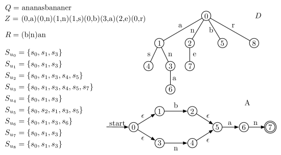
Figure 4: The compressed string $Z$ representing $Q$ and the corresponding dictionary trie $D$. The TNFA $A$ for the regular expression $R$ and the corresponding state-sets $S_{u_{i}}$ are given. The lastmatch pointers are as follows: $\mathrm{lastmatch}(s_{7},z_{i})=\{z_{0}\}$ for $i=0,1,\ldots,8$, $\mathrm{lastmatch}(s_{2},z_{i})=\mathrm{lastmatch}(s_{4},z_{i})=\mathrm{lastmatch}(s_{5},z_{i})=\{z_{3}\}$ for $i=3,6$, and $\mathrm{lastmatch}(s_{6},z_{i})=\{z_{2}\}$ for $i=2,7$. All other lastmatch pointers are $\bot$. Using the description we can find the matches: Since $s_{2}\in S_{u_{5}}$ the element $z_{3}\in M(s_{2},z_{6})$ represents the match $u_{6}+0pt(z_{3})-1=9$. The other matches can be found similarly.

An example description is shown in Fig. 4. The total size of the description for $z_{i}$ is $O(m)$ and therefore the space for all descriptions is $O(nm)$. In the next section we will show how to compute the descriptions. Assume for now that we have processed $z_{0},\ldots,z_{i-1}$. We show how to find the matches within $[u_{i},u_{i}+l_{i}-1]$. Given a state $s$ define $M(s,z_{i})=\{x_{1},\ldots,x_{k}\}$, where $x_{1}=\mathrm{lastmatch}(s,z_{i})$, $x_{j}=\mathrm{lastmatch}(s,\mathrm{parent}(x_{j-1}))$, $1<j\leq k$, and $\mathrm{lastmatch}(s,x_{k})=\bot$, i.e., $x_{1},\ldots,x_{k}$ is the sequence of ancestors of $z_{i}$ obtained by recursively following $\mathrm{lastmatch}$ pointers. By the definition of $\mathrm{lastmatch}$ and $M(s,z_{i})$ it follows that $M(s,z_{i})$ is the set of ancestors $x$ of $s$ such that $\bar{\delta}(s,x)\cap\Phi\neq\emptyset$. Hence, if $s\in S_{u_{i-1}}$ then each element $x\in M(s,z_{i})$ represents a match, namely, $u_{i}+0pt(x)-1$. Each match may occur for each of the $|S_{u_{i-1}}|$ states and to avoid reporting duplicate matches we use a priority queue to merge the sets $M(s,z_{i})$ for all $s\in S_{u_{i-1}}$, while generating these sets in parallel. A similar approach is used in [19]. This takes $O(\log m)$ time per match. Since each match can be duplicated at most $|S_{u_{i-1}}|=O(m)$ times the total time for reporting matches is $O(\mathit{occ}\cdot m\log m)$.

4.3 Computing Descriptions

Next we show how to compute descriptions efficiently. Let $1\leq\tau\leq n$ be a parameter. Initially, compute a set $C$ of compression elements according to Lemma 1 with parameter $\tau$. For each element $z_{j}\in C$ we store $l_{j}$ and the transition sets $\bar{\delta}(s,\mathrm{phrase}(z_{j}))$ for each state $s$ in $A$. Each transition set uses $O(m)$ space and therefore the total space used for $z_{j}$ is $O(m^{2})$. During the construction of $C$ we compute each of the transition sets by following the path of references to the nearest element $y\in C$ and computing state-set transitions from $y$ to $z_{j}$. By Lemma 1(ii) the distance to $y$ is at most $2\tau$ and therefore all of the $m$ transition sets can be computed in $O(\tau m^{2})$ time. Since, $|C|=O(n/\tau)$ the total preprocessing time is $O(n/\tau\cdot\tau m^{2})=O(nm^{2})$ and the total space is $O(n/\tau\cdot m^{2})$.

The descriptions can now be computed as follows. The integers $l_{i}$ and $u_{i}$ can be computed as before in $O(\tau)$ time. All $\mathrm{lastmatch}$ pointers for all compression elements can easily be obtained while computing the transitions sets. Hence, we only show how to compute the state-set values. First, let $S_{u_{0}}:=\{\theta\}$. To compute $S_{u_{i}}$ from $S_{u_{i-1}}$ we compute the path $p$ to $z_{i}$ from the nearest element $y\in C$. Let $p^{\prime}$ be the path from $z_{0}$ to $y$. Since $\mathrm{phrase}(z_{i})=\mathrm{label}(p^{\prime})\cdot\mathrm{label}(p)$ we can compute $S_{u_{i}}=\bar{\delta}(S_{u_{i-1}},\mathrm{phrase}(z_{i}))$ in two steps as follows. First compute the set

$$S^{\prime}=\bigcup_{s\in S_{u_{i-1}}}\bar{\delta}(s,\mathrm{phrase}(y))\;.$$ (1)

Since $y\in C$ we know the transition sets $\bar{\delta}(s,\mathrm{phrase}(y))$ and we can therefore compute the union in $O(m^{2})$ time. Secondly, we compute $S_{u_{i}}$ as the set $\delta(S^{\prime},\mathrm{label}(p))$. Since the distance to $y$ is at most $\tau$ this step uses $O(\tau m)$ time. Hence, all the state-sets $S_{u_{0}},\ldots,S_{u_{n}}$ can be computed in $O(nm(m+\tau))$ time.

4.4 Analysis

Combining it all, we have an algorithm using $O(nm(m+\tau)+\mathit{occ}\cdot m\log m)$ time and $O(nm+nm^{2}/\tau)$ space. Note that since we are using $\Omega(n)$ space, hashing is not needed and the algorithm works for ZLW as well. In summary, this completes the proof of Theorem 2.

4.5 Exploiting Word-level Parallelism

If we use the word-parallelism inherent in the word-RAM model, the algorithm of Navarro [19] uses $O(\left\lceil{m/w}\right\rceil(2^{m}+nm)+\mathit{occ}\cdot m\log m)$ time and $O(\left\lceil{m/w}\right\rceil(2^{m}+nm))$ space, where $w$ is the number of bits in a word of memory and space is counted as the number of words used. The key idea in Navarro’s algorithm is to compactly encode state-sets in bit strings stored in $O(\left\lceil{m/w}\right\rceil)$ words. Using a DFA based on a Glushkov automaton [10] to quickly compute state-set transitions, and bitwise OR and AND operations to compute unions and intersections among state-sets, it is possible to obtain the above result. The $O(\left\lceil{m/w}\right\rceil 2^{m})$ term in the above bounds is the time and space used to construct the DFA.

A similar idea can be used to improve Theorem 2. However, since our solution is based on Thompson’s automaton we do not need to construct a DFA. More precisely, using the state-set encoding of TNFAs given in [17, 6] a state-set transition can be computed in $O(\left\lceil{m/\log n}\right\rceil)$ time after $O(n)$ time and space preprocessing. Since state-sets are encoded as bit strings each transition set uses $\left\lceil{m/\log n}\right\rceil$ space and the union in (1) can be computed in $O(m\left\lceil{m/\log n}\right\rceil)$ time using a bitwise OR operation. As $n\geq\sqrt{u}$ in ZL78  and ZLW, we have that $\log n\geq\frac{1}{2}\log u$ and therefore Theorem 2 can be improved by roughly a factor $\log u$. Specifically, we get an algorithm using $O(n\left\lceil{m/\log u}\right\rceil(m+\tau)+\mathit{occ}\cdot m\log m)$ time and $O(nm\left\lceil{m/\log u}\right\rceil/\tau+nm)$ space.

References

- [1] A. V. Aho, R. Sethi, and J. D. Ullman. Compilers: principles, techniques, and tools. Addison-Wesley Longman Publishing Co., Inc., Boston, MA, USA, 1986.
- [2] A. Amir and G. Benson. Efficient two-dimensional compressed matching. In Proceedings of the 2nd Data Compression Conference, pages 279–288, 1992.
- [3] A. Amir and G. Benson. Two-dimensional periodicity and its applications. In Proceedings of the 3rd Symposium on Discrete algorithms, pages 440–452, 1992.
- [4] A. Amir, G. Benson, and M. Farach. Let sleeping files lie: pattern matching in Z-compressed files. J. Comput. Syst. Sci., 52(2):299–307, 1996.
- [5] P. Bille. New algorithms for regular expression matching. In Proceedings of the 33rd International Colloquium on Automata, Languages and Programming, pages 643–654, 2006.
- [6] P. Bille and M. Farach-Colton. Fast and compact regular expression matching, 2005. Submitted to a journal. Preprint availiable at arxiv.org/cs/0509069.
- [7] R. Cole and R. Hariharan. Approximate string matching: A simpler faster algorithm. SIAM J. Comput., 31(6):1761–1782, 2002.
- [8] M. Dietzfelbinger, A. Karlin, K. Mehlhorn, F. M. auf der Heide, H. Rohnert, and R. Tarjan. Dynamic perfect hashing: Upper and lower bounds. SIAM J. Comput., 23(4):738–761, 1994.
- [9] M. Farach and M. Thorup. String matching in Lempel-Ziv compressed strings. Algorithmica, 20(4):388–404, 1998.
- [10] V. M. Glushkov. The abstract theory of automata. Russian Math. Surveys, 16(5):1–53, 1961.
- [11] J. Kärkkäinen, G. Navarro, and E. Ukkonen. Approximate string matching on Ziv-Lempel compressed text. J. Discrete Algorithms, 1(3-4):313–338, 2003.
- [12] T. Kida, M. Takeda, A. Shinohara, M. Miyazaki, and S. Arikawa. Multiple pattern matching in LZW compressed text. In Proceedings of the 8th Data Compression Conference, pages 103–112, 1998.
- [13] G. M. Landau and U. Vishkin. Fast parallel and serial approximate string matching. J. Algorithms, 10(2):157–169, 1989.
- [14] V. Mäkinen, E. Ukkonen, and G. Navarro. Approximate matching of run-length compressed strings. Algorithmica, 35(4):347–369, 2003.
- [15] T. Matsumoto, T. Kida, M. Takeda, A. Shinohara, and S. Arikawa. Bit-parallel approach to approximate string matching in compressed texts. In Proceedings of the 7th International Symposium on String Processing and Information Retrieval, pages 221–228, 2000.
- [16] R. McNaughton and H. Yamada. Regular expressions and state graphs for automata. IRE Trans. on Electronic Computers, 9(1):39–47, 1960.
- [17] E. W. Myers. A four-russian algorithm for regular expression pattern matching. J. ACM, 39(2):430–448, 1992.
- [18] G. Navarro. A guided tour to approximate string matching. ACM Comput. Surv., 33(1):31–88, 2001.
- [19] G. Navarro. Regular expression searching on compressed text. J. Discrete Algorithms, 1(5-6):423–443, 2003.
- [20] G. Navarro, T. Kida, M. Takeda, A. Shinohara, and S. Arikawa. Faster approximate string matching over compressed text. In Proceedings of the Data Compression Conference (DCC ’01), page 459, Washington, DC, USA, 2001. IEEE Computer Society.
- [21] G. Navarro and M. Raffinot. A general practical approach to pattern matching over Ziv-Lempel compressed text. Technical Report TR/DCC-98-12, Dept. of Computer Science, Univ. of Chile., 1998.
- [22] P. Sellers. The theory and computation of evolutionary distances: Pattern recognition. J. Algorithms, 1:359–373, 1980.
- [23] K. Thompson. Programming techniques: Regular expression search algorithm. Commun. ACM, 11:419–422, 1968.
- [24] T. A. Welch. A technique for high-performance data compression. IEEE Computer, 17(6):8–19, 1984.
- [25] J. Ziv and A. Lempel. A universal algorithm for sequential data compression. IEEE Trans. Inform. Theory, 23(3):337–343, 1977.
- [26] J. Ziv and A. Lempel. Compression of individual sequences via variable-rate coding. IEEE Trans. Inform. Theory, 24(5):530–536, 1978.