In presenting this thesis in partial fulfillment of the requirements for an advanced degree at the University of British Columbia, I agree that the Library shall make it freely available for reference and study. I further agree that permission for extensive copying of this thesis for scholarly purposes may be granted by the head of my department or by his or her representatives. It is understood that copying or publication of this thesis for financial gain shall not be allowed without my written permission.

  

Department of Physics and Astronomy

The University of British Columbia

6224 Agricultural Road

Vancouver, B.C., Canada

V6T 1Z1

Date:

  

Abstract

We perform a numerical study of the critical regime for the general relativistic collapse of collisionless matter in spherical symmetry. The evolution of the matter is given by the Vlasov equation (or Boltzmann equation) and the geometry by Einstein’s equations. This system of coupled differential equations is solved using a particle-mesh (PM) method. This method approximates the distribution function which describes the matter in phase space with a set of particles moving along the characteristics of the Vlasov equation. The individual particles are allowed to have angular momentum different from zero but the total angular momentum has to be zero to retain spherical symmetry.

In accord wih previous work by Rein, Rendall and Schaeffer, our results give some indications that the critical behaivour in this model is of Type I (the smallest black hole in each family has a finite mass). For the families of initial data that we have studied it seems that in the critical regime the solution is a static spacetime with non-zero radial momentum for the individual particles. We have also found evidence for scaling laws for the time that the critical solutions spend in the critical regime.

Table of Contents

toc

List of Tables

lot

List of Figures

lof

Acknowledgements

I want to thank the rest of the graduate students under the supervision of Matt Choptuik, especially Jason Ventrella, with whom I have had many useful discussions. I also want to thank Bojan Losic, Noureddine Hambli, Luis Lehner and Bill Unruh who have been there for any question I ever had. I am grateful to all the people who have encouraged me from Spain, my family and friends, and the people of the department of Theoretical Physics and History of Science in the University of the Basque Country who allowed me to work there for some time during the development of this thesis. Finally, my supervisor, Matt Choptuik, for keeping on asking me where are the particles? and for being a friend in addition to a supervisor.

Chapter 1 Introduction

1.1 Gravitation and Critical Phenomena

Einstein’s theory of gravitation connects the geometry of spacetime to its matter content via the field equations:

$$G_{ab}=8\pi T_{ab}.$$ (1.1)

Here $G_{ab}$ is the Einstein tensor, whose coefficients are complicated functions of the metric, $g_{ab}$, and its first and second derivatives. $T_{ab}$ is the stress energy tensor, which depends on the matter, and also, in general, on the metric.

In a given coordinate system, these equations are non-linear partial differential equations for the metric coefficients and can give rise to very interesting solutions for the spacetime. Some of the most interesting phenomena occur at the threshold of black hole formation as was first discovered numerically by Choptuik [1], who studied the collapse of a massless scalar field in spherical symmetry.

For initial data characterized by one parameter $p$ (the maximum amplitude of the scalar field for example), Choptuik found a critical value $p^{*}$ such that for values of $p$, $p>p^{*}$, the evolution gave rise to the formation of a black hole, while for $p<p^{*}$ the scalar field dispersed to infinity. Near $p=p^{*}$ the space-time approached a universal solution, independent of the particular choice of the initial shape of the pulse (e.g. gaussian, tanh, etc). It was found that the near-critical dynamics was characterized by self-similar oscillations with scaling factor $e^{\Delta}$.

Choptuik also found that the masses of the black hole formed obeyed a scaling law:

$$M_{BH}\propto|p-p^{*}|^{\gamma}$$ (1.2)

where $\gamma$ was a universal exponent, again, universal in the sense of being independent of the choice of the family of initial data. This equation shows that, in principle, one can form black holes with arbitrarily small masses in the model. The transition to black hole formation in this case is thus continuous in the mass of the black hole. In analogy with the critical behavior in statistical mechanics this was called a Type II critical solution.

A lot of work has been done in the last few years trying to find the critical solutions for different types of matter. Type I transitions (i.e. transitions where the mass of the smaller black hole is finite) have been also found [2]. In this case, the solutions that have been found are either static or periodic [3]. Here it was found that the time that the solution stays in the critical regime scales like:

$$\tau\sim-\sigma\ln{|p-p^{*}|}$$ (1.3)

where, again, $\sigma$ is a universal constant.

The process of tuning $p$ to $p^{*}$ can be understood as choosing initial data such that at the threshold of black hole formation, we tune-out any growing component. Since we can tune away the growing components using only one parameter, the solution apparently has exactly one unstable mode. Linear perturbations of the critical solutions [3] agree with that observation.

In this thesis we study the critical regime for collisionless matter in spherical symmetry. If we think of the matter as being composed of individual particles, allowing these particles to have angular momentum different from zero (keeping the net angular momentum equal to zero to remain in spherical symmetry) can give us some insight concerning the importance of angular momentum in critical phenomena, without needing to go to spacetimes with less symmetry.

1.2 Collisionless Matter (A little bit of history)

Collisionless matter (or dust) has been widely studied in general relativity. Einstein [4] used this type of matter to investigate the physical significance of the singularity at $r=2\,M$ for the Schwarzschild solution. He studied clusters of particles rotating in circular orbits (and spherical symmetry) and proved that for clusters in equilibrium the Schwarzschild mass function cannot reach $M(r)=r/2$ ($r$ being the areal coordinate), therefore these configurations cannot have an event horizon nor a singularity. He postulated that this result also would hold for systems not in equilibrium and concluded that in “physical reality” there is no configuration of matter such that $M(r)=r/2$ (i.e. black holes cannot form). Although he came to the wrong conclusion, he studied one of the first models for relativistic stars.

In the case when the angular momentum of each particle is zero, and the spacetime is spherically symmetric, Oppenheimer and Snyder [5] showed that a homogeneous distribution of this kind of matter generally forms a singularity. Using comoving coordinates they found the solution for the spacetime and deduced that singularity formation would happen in finite proper time (at least from the point of view of the comoving observers). Tolman [6] and Bondi [7] generalized this result for non-homogeneous configurations, restricting to the case where no particle overtakes any other during the evolution.

Eardley and Smarr [8] considered the same model as Tolman and Bondi and studied the existence of maximal ($K=0$) and constant mean curvature ($K=K_{o}$) slicing conditions. Shapiro and Teukolsky [9], [10], [11], [12], [13] have studied this system in detail in the context of models of stellar clusters. They developed a code very similar to ours to study properties of relativistic clusters, such as stability and collapse to a black hole. They also extended the code to treat more general spacetimes , i.e. with axial symmetry, [14] to study naked singularities.

Rendall [16], [17], and Rein [15] have a series of papers addressing general properties for the Einstein-Vlasov system (the Cauchy problem, existence of static solutions in spherical symmetry, existence of general asymptotically flat solutions, etc…).

More recently, Rendall, Rein and Schaeffer [18] have published the first study of critical behavior (black-hole threshold behavior) for this type of matter. Indeed, in this last paper Rendall et al argue that the critical solution in the case of collisionless matter is generically Type I. Our results agree with theirs in that we also find evidence for Type I transitions for certain initial data families which we have studied in this thesis. In addition to that result, we argue here that the critical solutions in this model are static, and we present evidence for scaling laws of the form (1.3). Finally we have preliminary investigations aimed at determining whether the critical solution is unique (universality).

Chapter 2 The Equations

The dynamical state of dust can be described by a distribution function, $f$:

$$f(x^{a},p_{a})=dN/dV_{p}$$ (2.1)

where $N$ is the number of particles and $V_{p}$ is the volume in phase space. In our case, and since the matter is collisionless, the volume in phase space is a conserved quantity during the evolution of the system (Liouville theorem). This implies that the distribution function is also a conserved quantity:

$$\frac{df}{d\tau}=0$$ (2.2)

This is the collisionless Boltzmann or Vlasov equation. This equation plus Einstein’s equations (1.1), all restricted to spherical symmetry, i.e.:

$$f(t,x^{i},p_{i})=f(t,R\,x^{i},R\,p_{i})\quad{\mathrm{with}}\quad R\in SO(3)\quad i=1,2,3$$ (2.3)

form the system of equations that we want to solve numerically.

Numerical solutions of PDEs generally involves discretization of the continuum problem, and here we can consider at least two approaches: 1) Consider a set of particles which approximates the distribution function at the initial time and evolve the particles along the characteristics of equation (2.2). The geometry is computed at each time step using the energy densities derived from the positions and velocities of the particles. 2) Discretize the Vlasov equation for the distribution function in phase space and solve for it directly in phase space. In this case the energy densities, required in the update of the geometry, are calculated by integrating the distribution function over momentum space.

In the particle approach, we have the problem that a given set of particles is just one of the infinite number of possible realizations for given density and velocity profiles, therefore we introduce statistical errors. In the second case we have to solve the Vlasov equation, a partial differential equation in phase space. Although we have taken the particle approach due to the simplicity of the evolution equations, we include the equations for the direct integration in Appendix B.

As with any problem in “3+1” (or ADM) numerical relativity, we want to be able to specify initial data on a spatial hypersurface and then evolve these data in time. To do this, we need to split the equations (1.1) into a set of constraint equations (equations that must be satisfied at each instant of time) and dynamical or evolution equations (equations that tell us how to evolve the geometric quantities in time). In the most general case, we will have four constraint and six second-order-in-time evolution equations.

In order to do this splitting, we will make use of the $3+1$ formalism due to Arnowitt, Deser and Misner (ADM), for a review of this formalism see [19]. We have followed a summary by Choptuik [20] which is itself based on a review by York [24].

In the remainder of this chapter, we derive the system of equations that we solve. We start with a summary of the $3+1$ formalism and its restriction to the spherical symmetric case, and a definition and description of the maximal-areal coordinate system. In section 2.2 we explain how the Einstein’s equations are coupled to the matter, and in 2.3 we explain the particle evolution equations in our coordinates. The chapter ends with some calculations of conserved quantities.

2.1 The 3+1 Formalism of General Relativity.

We consider a spacetime manifold with metric $g_{ab}$ defined on it, and assume that we can slice the manifold into spacelike hypersurfaces, defined by $t=$ constant, where $t$ is our time coordinate. At least locally then, the space-like surfaces can be described in terms of a closed one-form, $\Omega_{a}$, which is just the gradient of $t$

$$\Omega_{a}=dt=\nabla_{a}t.$$ (2.4)

The norm of this one-form is:

$$g^{ab}\Omega_{a}\Omega_{b}=-\alpha^{-2},$$ (2.5)

where $\alpha$ is a scalar function commonly known as the lapse function. As long as our slices are spacelike, $\alpha$ will be strictly positive. We introduce a normalized one-form, $n_{a}$, defined by

$$n_{a}=-\alpha\Omega_{a}=-\alpha\nabla_{a}t.$$ (2.6)

The contravariant vector, $n^{a}=g^{ab}n_{b}$, which is the future-directed normal to the surfaces, can be viewed as the four velocity field of observers moving orthogonally to the slices.

In this section, again following York, we will describe the 3+1 split in terms of 4-dimensional tensors. At the same time, we will need to decompose various tensors (including the Einstein and stress energy tensors appearing in (1.1)) into pieces parallel to $n^{a}$ (“timelike” pieces) and pieces orthogonal to $n^{a}$ (“spacelike” pieces). Thus we define

$$W^{n}=-W^{a}n_{a},$$ (2.7)

where the sign convention is again York’s, while for covariant vectors we define

$$W_{n}=W_{a}n^{a}.$$ (2.8)

For the projection onto the hypersurfaces we use the projection operator:

$$\gamma^{a}{}_{b}=\delta^{a}{}_{b}+n^{a}n_{b}$$ (2.9)

The projection of the space-time metric to the hypersurfaces is:

$$\gamma_{ab}=\gamma^{c}{}_{a}\gamma^{d}{}_{b}\,g_{cd}=g_{ab}+n_{a}\,n_{b}$$ (2.10)

and is, in fact, the metric induced on the hypersurfaces by the 3+1 splitting. (Note that $\gamma^{ab}$ is not necessarily the inverse of $\gamma_{ab}$, as follows immediately from the definition of $\gamma^{a}{}_{b}$, and in this section we raise and lower all indexes with the four dimensional metric $g^{ab}$ and its inverse). We can now introduce the natural derivative operator on the space-like surfaces, by projection of the four dimensional covariant derivative:

$$D_{a}=\gamma^{b}{}_{a}\,\nabla_{b}.$$ (2.11)

It is easily shown that this derivative is compatible with the spatial metric:

$$D_{a}\gamma_{bc}=0.$$ (2.12)

Having defined a derivative operator on the hypersurfaces, we can compute the associated Riemann tensor ${{{}^{3}{\cal R}}_{abc}}^{d}$ which measures the intrinsic curvature of the hypersurface. For example, for a spatial one form $\omega_{a}$ ($\omega_{a}n^{a}=0$) we have

$$\left(D_{a}D_{b}-D_{b}D_{a}\right)\omega_{c}={{{}^{3}{\cal R}}_{abc}}^{d}\omega_{d}.$$ (2.13)

We can then also define the spatial Ricci tensor, ${{}^{3}{\cal R}}_{ac}={{{}^{3}{\cal R}}_{abc}}^{b}$ and the spatial Ricci scalar, ${}^{3}{\cal R}={{{}^{3}{\cal R}}^{a}}_{a}$.
Finally, we define the extrinsic curvature tensor, $K_{ab}$:

$$K_{ab}=-D_{a}n_{b}=\nabla_{a}n_{b}-n_{a}a_{b},$$ (2.14)

where $a_{b}=n^{a}D_{a}n_{b}$ is the dual to the four acceleration field of the observers moving with the slicing.
The geometry of the space-time is completely defined by the spatial metric, $\gamma_{ab}$, which describes the geometry of each slice, and the extrinsic curvature tensor which tells us how each slice is embedded in the four dimensional space-time.

We can write Einstein’s equations in terms of the tensors defined above, as well as the following projections of the stress energy tensor:

$$\rho = T^{ab}n_{a}n_{b}$$ (2.15)

$$j^{a} = \gamma^{a}{}_{b}(T^{bc}n_{c})$$ (2.16)

$$S^{ab} = \gamma^{a}{}_{c}\gamma^{b}{}_{d}T^{cd}$$ (2.17)

These are interpreted as the local energy density, momentum density and spatial stress tensor, respectively, for an observer moving orthogonally to the space-like hypersurfaces.
The Hamiltonian constraint is found by contracting Einstein’s equations with $n^{a}$ twice, $G_{ab}n^{a}n^{b}=T_{ab}n^{a}n^{b}$, yielding

$${{}^{3}{\cal R}}+K^{2}-{K^{a}}_{b}{K^{b}}_{a}=16\pi\rho$$ (2.18)

where $K=g^{ab}\,K_{ab}=\gamma^{ab}\,K_{ab}$ is the trace of the extrinsic curvature and ${{}^{3}\cal R}$ is the spatial Ricci scalar defined previously.
If we contract Einstein’s equations once with $n^{a}$, and then project the resulting vector onto the hypersurface, $\gamma^{a}{}_{c}\,G^{cb}\,n_{b}=\gamma^{a}{}_{c}T^{cb}n_{b}$, we get the momentum constraint:

$$D_{b}K^{ab}-D^{a}K=8\pi j^{a}.$$ (2.19)

These two constraint equations involve only spatial tensors and spatial derivatives of spatial tensors, and must be satisfied on each spacelike slice, including the initial slice.

In order to derive the evolution equations we use the Lie derivative along the vector field, $N^{a}$:

$$N^{a}=\alpha n^{a}+\beta^{a}=d/dt$$ (2.20)

where $\beta^{a}$ is an arbitrary spatial vector field, commonly known as the shift vector. Note that $N^{a}$ satisfies:

$$N^{a}\Omega_{a}=1$$ (2.21)

It can be shown that Lie differentiation along $N^{a}$ commutes with the projection operator. We can now write the rest of equations (1.1) as two different sets: (1) the evolution of the spatial metric:

$${\cal L}_{t}\gamma_{ab}=-2\alpha K_{ab}+{\cal L}_{\beta}\gamma_{ab}$$ (2.22)

which can also be viewed as a definition of $K_{ab}$, and (2) the evolution equations for the extrinsic curvature:

$${\cal L}_{t}{K^{a}}_{b}={\cal L}_{\beta}{K^{a}}_{b}-D^{a}D_{b}\alpha+\\ \alpha{{}^{3}{\cal R}^{a}}_{b}+K{K^{a}}_{b}+8\pi\left(\frac{1}{2}{P^{a}}_{b}\left(S-\rho\right)-{S^{a}}_{b}\right)$$ (2.23)

where $S$ is the trace of tensor given by equation (2.17).

2.1.1 3+1 Formalism in Spherical Symmetry

We now restrict our attention to spherical symmetry. In contrast to the previous section, where our tensor expressions involved abstract 4-dimensional indices, we will be mostly concerned with the components of specific 3-tensors in this section. Thus, Latin indices $i,j,k,\cdots$ range over the spatial values $1,2$ and $3$, and all indices of the spatial tensors are raised and lowered with $\gamma^{ij}$ and $\gamma_{ij}$ respectively, where $\gamma^{ij}\,\gamma_{jk}=\delta^{i}{}_{k}$.

The most general 3-metric in spherical symmetry can be written as:

$${}^{3}d{s}^{2}=a^{2}\left(t,r\right)\,dr^{2}+r^{2}\,b^{2}\left(t,r\right)\,d\Omega^{2}$$ (2.24)

where $d\Omega^{2}$ is the metric on the unit sphere, $d\Omega^{2}=d\theta^{2}+\sin^{2}{\theta}\,d\phi^{2}$. From the 3-metric, we can compute the associated connection coefficients or Christoffel symbols:

$$\Gamma^{i}{}_{jk}=\frac{1}{2}\gamma^{in}\left(\gamma_{nj,k}+\gamma_{nk,j}-\gamma_{jk,n}\right)$$ (2.25)

In our coordinates, the non-zero connection coefficients are:

$$\begin{array}[]{c}\begin{array}[]{lll}\Gamma^{r}{}_{rr}=a^{\prime}/a&\quad\quad\Gamma^{r}{}_{\theta\theta}=-\left(\left(r^{2}b^{2}\right)^{\prime}\right)/\left(2a^{2}\right)&\Gamma^{r}{}_{\phi\phi}=-\sin^{2}{\theta}\left(r^{2}b^{2}\right)^{\prime}/\left(2a^{2}\right)\\ \end{array}\\ \\ \begin{array}[]{ll}\Gamma^{\theta}{}_{r\theta}=\left(\left(r^{2}b^{2}\right)^{\prime}\right)/\left(2r^{2}b^{2}\right)&\quad\quad\quad\Gamma^{\theta}{}_{\phi\phi}=-\sin{\theta}\cos{\theta}\\ \\ \Gamma^{\phi}{}_{r\phi}=\left(r^{2}b^{2}\right)^{\prime}/\left(2r^{2}b^{2}\right)&\quad\quad\quad\Gamma^{\phi}{}_{\theta\phi}=\cot{\theta}\end{array}\end{array}$$ (2.26)

We also need to compute the components of the Ricci tensor:

$${}^{3}R_{ij}=\Gamma^{n}{}_{ij,n}-\Gamma^{n}{}_{in,j}+\Gamma^{n}{}_{nm}\,\,\Gamma^{m}{}_{ij}-\Gamma^{n}{}_{jm}\,\,\Gamma^{m}{}_{in}$$ (2.27)

from which we find the non-zero components:

$$\begin{array}[]{l}{}^{3}R_{rr}=-\left[\left(r^{2}b^{2}\right)^{\prime}/\left(r^{2}b^{2}\right)\right]^{\prime}+a^{\prime}\left(r^{2}b^{2}\right)^{\prime}/\left(ar^{2}b^{2}\right)-\frac{1}{2}\left[\left(r^{2}b^{2}\right)^{\prime}/\left(r^{2}b^{2}\right)\right]^{2}\\ \\ {}^{3}R_{\theta\theta}=-\left[\left(r^{2}b^{2}\right)^{\prime}/\left(2a^{2}\right)\right]^{\prime}+1-\left[a^{\prime}\left(r^{2}b^{2}\right)^{\prime}/\left(2a^{3}\right)\right]\\ \\ {}^{3}R_{\phi\phi}=\sin^{2}{\theta}R_{\theta\theta}\end{array}$$ (2.28)

The mixed components are given by

$$\begin{array}[]{c}{}^{3}R^{r}{}_{r}=-2\left[\left(rb\right)^{\prime}/a\right]^{\prime}/\left(arb\right)\\ \\ {}^{3}R^{\theta}{}_{\theta}=R^{\phi}{}_{\phi}=\left[a-\left(rb\left(rb\right)^{\prime}/a\right)^{\prime}\right]/\left(a\left(rb\right)^{2}\right).\end{array}$$ (2.29)

Another quantity which we need is ${\alpha_{|i}}^{|j}$, where “$|$” denotes covariant differentiation with respect to the 3-metric.

$${\alpha_{|i}}^{|j}=\gamma^{jk}\left(\alpha_{,ik}-\Gamma^{n}{}_{ik}\,\alpha_{,jn}\right)$$ (2.30)

which has the following non-zero components:

$$\begin{array}[]{lcr}{\alpha_{|r}}^{|r}=\left(\alpha^{\prime}/a\right)^{\prime}/a&{\alpha_{|\theta}}^{|\theta}=\alpha^{\prime}\left(r^{2}b^{2}\right)^{\prime}/\left(2r^{2}a^{2}b^{2}\right)&{\alpha_{|\phi}}^{|\phi}=\left(rb\right)^{\prime}\alpha^{\prime}/\left(rba^{2}\right)\end{array}$$ (2.31)

Finally, the Ricci scalar, ${}^{3}R=\gamma^{ij}R_{ij}$, is given by:

$${}^{3}R=\frac{2}{arb}\left[-2\left(\frac{\left(rb\right)^{\prime}}{a}\right)^{\prime}+\frac{a}{rb}\left(1-\frac{{\left(rb\right)^{\prime}}^{2}}{a^{2}}\right)\right]$$ (2.32)

At this point we have calculated all the geometric objects intrinsic to the spatial slices that we need. Now, we embed these slices into the most general spherically symmetric spacetime whose metric can be written:

$$ds^{2}=\left(-\alpha^{2}+a^{2}\beta^{2}\right)dt^{2}+2a^{2}\beta dtdr+a^{2}dr^{2}+r^{2}b^{2}d\Omega^{2}$$ (2.33)

where $\alpha$, $\beta$, $a$ and $b$ are all functions of $r$ and $t$. Note that due to the spherical symmetry, the shift vector has only a radial component; $\beta^{i}=\left(\beta,0,0\right)$, so $\beta$ will be called the shift function. In these coordinates $n_{\mu}=\left(-\alpha,0,0,0\right)$ and $n^{\mu}=\left(1/\alpha,-\beta/\alpha,0,0\right)$.

The extrinsic curvature can be written in terms of the 4-metric coefficients:

$$K_{ij}=-\frac{1}{2\alpha}\left(\frac{\partial\gamma_{ij}}{\partial t}-\gamma_{ij,k}\beta^{k}-\gamma_{ik}\beta^{k}{}_{,j}-\gamma_{kj}\beta^{k}{}_{,i}\right)$$ (2.34)

From this we compute the non-vanishing components for the current spherically symmetric case:

$$K_{rr} = \frac{a}{\alpha}\left(\left(a\beta\right)^{\prime}-\dot{a}\right)$$ (2.35)

$$K_{\theta\theta} = \frac{rb}{\alpha}\left(\beta\left(rb\right)^{\prime}-r\dot{b}\right)$$ (2.36)

$$K_{\phi\phi} = \sin^{2}{\theta}K_{\theta\theta}$$ (2.37)

The corresponding components with mixed indexes are:

$$K^{r}{}_{r} = \frac{1}{a\alpha}\left(\left(a\beta\right)^{\prime}-\dot{a}\right)$$ (2.38)

$$K^{\theta}{}_{\theta} = \frac{1}{rb\alpha}\left(\beta\left(rb\right)^{\prime}-r\dot{b}\right)$$ (2.39)

$$K^{\phi}{}_{\phi} = K^{\theta}{}_{\theta}$$ (2.40)

and the trace of the extrinsic curvature is

$$K=\frac{1}{a\alpha}\left(\left(a\beta\right)^{\prime}-\dot{a}\right)+\frac{2}{\alpha}\left(\beta\frac{\left(rb\right)^{\prime}}{rb}-\frac{\dot{b}}{b}\right)$$ (2.41)

Finally, the only non-zero component of $D_{i}K\equiv K_{|i}$ is

$$K_{|r}=K_{,r}=-\frac{1}{a\alpha}\left(\frac{a^{\prime}}{a}+\frac{\alpha^{\prime}}{\alpha}\right)\left(a\beta^{\prime}-\dot{a}\right)+\frac{1}{a\alpha}\left((a\beta)^{\prime\prime}-\dot{a}^{\prime}\right)-\frac{2}{\alpha^{2}}\alpha^{\prime}\left(\beta\frac{(rb)^{\prime}}{rb}-1\right)$$

2.1.2 Maximal Areal Coordinate System.

Einstein’s equations allow for coordinate freedom that we need to fix. We have chosen maximal-areal coordinates (defined below), but have also included the equations for the polar-areal system in Appendix C. The main advantage of maximal-areal coordinates is that, in contrast to the polar-areal case, the slices used can penetrate apparent horizons. As the name suggests, in the maximal-areal coordinate system, the radial coordinate is areal, so that the proper area of 2-spheres with radius $r$ is $4\pi r^{2}$. In terms of the general spherically-symmetric 4-metric (2.33), this means that $b\left(r,t\right)\equiv 1$. The time coordinate is fixed by demanding that the 3-slices be maximal, i.e. that $K\left(r,t\right)=0$. This leads to a condition on the lapse function $\alpha\left(r,t\right)$ (the so-called slicing condition), which must be satisfied at each instant of time.

Thus, in maximal-areal coordinates the 4-metric (2.33) takes the form:

$$ds^{2}=\left(-\alpha^{2}+a^{2}\beta^{2}\right)dt^{2}+2a^{2}\beta dtdr+a^{2}dr^{2}+r^{2}d\Omega^{2}$$ (2.42)

Using the expressions we derived in the previous section, we compute the relevant geometrical quantities we need in order to write Einstein’s equations in terms of these metric coefficients:

$$\begin{array}[]{c}R=2\left[-2\left(1/a\right)^{\prime}+a/r\left(a-1/a^{2}\right)\right]/(a\,r)\\ \\ \begin{array}[]{ll}R^{r}{}_{r}=-2\left(1/a\right)^{\prime}/(a\,r)&R^{\theta}{}_{\theta}=R^{\phi}{}_{\phi}=\left[a-\left(r/a\right)^{\prime}\right]/(a\,r^{2})\\ \\ K^{r}{}_{r}=\left(\left(a\,\beta\right)^{\prime}-\dot{a}\right)/(a\,\alpha)&K^{\theta}{}_{\theta}=K^{\phi}{}_{\phi}=\beta/\left(r\,\alpha\right)\\ \\ {K^{i}{}_{r}}{}_{|i}=K^{r}{}_{r,r}+2\left(K^{r}{}_{r}-K^{\theta}{}_{\theta}\right)/r&K_{|r}=0\\ \\ {\alpha_{|r}}^{|r}=\left(\alpha^{\prime}/a\right)^{\prime}/a&{\alpha_{|\theta}}^{|\theta}={\alpha_{|\phi}}^{|\phi}=\alpha^{\prime}/\left(r\,a^{2}\right)\end{array}\end{array}$$ (2.43)

We can now specialize equations (1.1):

Hamiltonian Constraint:

$$\frac{a^{\prime}}{a}=\frac{3}{2}a^{2}r{K^{\theta}{}_{\theta}}^{2}+4\pi ra^{2}\rho+\frac{1}{2r}\left(1-a^{2}\right)$$ (2.44)

Momentum Constraint:

$${K^{\theta}{}_{\theta}}^{\prime}=-\frac{3}{r}K^{\theta}{}_{\theta}-4\pi j_{r}$$ (2.45)

Evolution of the 3-metric:

$$\dot{a} = 2\alpha aK^{\theta}{}_{\theta}+\left(a\beta\right)^{\prime}$$ (2.46)

$$\beta = \alpha rK^{\theta}{}_{\theta}$$ (2.47)

Slicing Condition:

$$\alpha^{\prime\prime}=\alpha^{\prime}\left(\frac{a^{\prime}}{a}-\frac{2}{r}\right)+\frac{2\alpha}{r^{2}}\left(2r\frac{a^{\prime}}{a}+a^{2}-1\right)+4\pi a^{2}\alpha\left(S-3\rho\right)$$ (2.48)

where in deriving the last formula, we have made use of the slicing condition ($K=0$), and the evolution equations for the extrinsic curvature components, equations (2.23). As we will discuss in more detail below, we have chosen to do a constrained evolution, which, in this case means that we use the constraint equations, rather than evolution equations, to update $a$ and $K^{\theta}{}_{\theta}$.

2.2 Stress-Energy Tensor

In this section we explain how we calculate the energy densities $\rho$, $j_{r}$ and $S$ that appear in equations (2.44-2.48). We approximate the distribution function (2.1) by a set of $N$ “spherical particles”. Since the particles only interact with each other gravitationally, we have

$$T^{\mu\nu}=\sum_{i=1}^{N}T^{\mu\nu}_{i}$$ (2.49)

where $T^{\mu\nu}_{i}$ is the stress energy tensor for a single particle. For a point particle we can write:

$$T^{\mu\nu}_{i}=\frac{p^{\mu}_{i}\,p^{\nu}_{i}}{m_{i}}\delta(\vec{r}-\vec{r}_{i}(t)).$$ (2.50)

Here, $p^{\mu}_{i}$ is the $\mu$ component of the 4 momentum of the $i$-th particle, $m_{i}$ is its rest mass, and $\vec{r}_{i}(t)$ is the spatial position of the particle at time t.

Using equations (2.15-2.17) for $\rho$, $S$ and $j_{r}$ specialized to our coordinates, we get:

$$\left[\rho\right]_{i} = \alpha^{2}\left[T^{tt}\right]_{i}$$ (2.51)

$$\left[S\right]_{i} = \frac{1}{a^{2}}\left[T_{rr}\right]_{i}+\frac{1}{r^{2}}\left[T_{\theta\theta}\right]_{i}+\frac{1}{r^{2}{\mathrm{s}in}^{2}{\theta}}\left[T_{\phi\phi}\right]_{i}$$ (2.52)

$$\left[j_{r}\right]_{i} = \alpha\left[T^{t}{}_{r}\right]_{i}$$ (2.53)

Now we relax the point particle approximation and assume that each particle is a spherically symmetric shell of mass, uniformly distributed over a region $\Delta r$ of space. These shells of matter are averages of the shells at that point with magnitude of the angular momentum $l$ pointing in all posible directions. Therefore the angular momentum of the average is zero, $\vec{l}=0$, but $l^{2}\neq 0$. The proper volume that each particle occupies is then:

$$V_{i}=\frac{p^{t}}{m_{i}}\,\Delta r\int\sqrt{-g}\,\,d\phi\,d\theta=4\pi\,\Delta r\,\alpha\,a\,\frac{r^{2}_{i}\,\,p^{t}_{i}}{m_{i}}$$ (2.54)

and we can approximate the delta function that appears in (2.50) by $1/V_{i}$. This yields:

$$\rho_{i} = \frac{1}{4\pi\Delta ra}\frac{\left[\bar{p}^{t}\right]_{i}}{r^{2}_{i}}$$ (2.55)

$$S_{i}=\left[S^{r}{}_{r}\right]_{i}+\left[S^{a}{}_{a}\right]_{i} = \frac{1}{4\pi\Delta ra^{3}}\frac{{\left[p_{r}\right]_{i}}^{2}}{\left[\bar{p}^{t}\right]_{i}r^{2}_{i}}+\frac{1}{4\pi\Delta ra}\frac{\left[l\right]^{2}_{i}}{r^{4}_{i}\left[\bar{p}^{t}\right]_{i}}$$ (2.56)

$$\left[j_{r}\right]_{i} = \frac{1}{4\pi\Delta ra}\frac{\left[p_{r}\right]_{i}}{r^{2}_{i}}$$ (2.57)

Here $a$, $\alpha$ and $\beta$ are evaluated at $r=r_{i}$, $\left[\bar{p}^{t}\right]_{i}$ is defined as $\left[\bar{p}^{t}\right]_{i}\equiv\alpha\left[p^{t}\right]_{i}$, and ${\left[l\right]_{i}}^{2}\equiv{\left[p_{\theta}\right]_{i}}^{2}+{\left[p_{\phi}\right]_{i}}^{2}/\sin^{2}{\theta_{i}}$ is the square of the magnitude of the angular momentum of the $i$-th particle. We then introduce quantities which do not explicitly depend on the geometry (since after updating the particle positions we want to solve for the geometry): $\left[\bar{\rho}\right]_{i}\equiv a\left[\rho\right]_{i}$, $\left[\bar{S}^{r}{}_{r}\right]_{i}\equiv a^{3}\left[S^{r}{}_{r}\right]_{i}$, $\left[\bar{S}^{a}{}_{a}\right]_{i}=a\left[S^{a}{}_{a}\right]_{i}$ and $\left[\bar{\j}_{r}\right]_{i}\equiv a\left[j_{r}\right]_{i}$.

We interpolate the one-particle quantities to the continuum and sum over all the particles to find the total values:

$$\bar{f}=\sum_{i=1}^{N_{p}}\bar{f}_{i}W(r-r_{i})$$ (2.58)

where $\bar{f}_{i}$ is any of the barred quantities defined above for each particle, $\bar{f}$ is the corresponding quantity in the continuum case, and $W(r-r_{i})$ is an interpolation function (see section 3.4 for further explanation of how we define this function). Having defined (2.58) we can now write equations (2.44-2.48) as

$$\frac{a^{\prime}}{a} = \frac{1-a^{2}}{2r}+\frac{3}{2}ra^{2}{K^{\theta}{}_{\theta}}^{2}+4\pi ar\bar{\rho}$$ (2.59)

$${K^{\theta}{}_{\theta}}^{\prime} = -\frac{3}{r}K^{\theta}{}_{\theta}-4\pi\frac{\bar{\j}_{r}}{a}$$ (2.60)

$$\alpha^{\prime\prime} = \alpha^{\prime}\left(\frac{a^{\prime}}{a}-\frac{2}{r}\right)+\frac{2\alpha}{r^{2}}\left(a^{2}-1+2r\frac{a^{\prime}}{a}\right)+4\pi a\alpha\left(\frac{\bar{S}^{r}{}_{r}}{a^{2}}+\bar{S}^{a}{}_{a}-3\bar{\rho}\right)$$ (2.61)

$$\beta = \alpha rK^{\theta}_{\theta}$$ (2.62)

2.3 Evolution Equations

The equations of motion for the particles are just the geodesic equations (the characteristics of the Vlasov equation). These can be expressed in terms of the four momentum of the particle:

$$p^{a}\nabla_{a}p^{b}=0,$$ (2.63)

so in our coordinate system we have:

$$\frac{dp^{t}}{d\tau} = -\Gamma^{t}{}_{tt}\,\left({p^{t}}\right)^{2}-2\Gamma^{t}{}_{tr}\,p^{r}p^{t}-\Gamma^{t}{}_{rr}\,\left({p^{r}}\right)^{2}-\Gamma^{t}{}_{\theta\theta}\,\frac{l^{2}}{r^{4}}$$ (2.64)

$$\frac{dp^{r}}{d\tau} = -\Gamma^{r}{}_{tt}\,\left({p^{t}}\right)^{2}-2\Gamma^{r}{}_{tr}\,p^{r}p^{t}-\Gamma^{r}{}_{rr}\,\left({p^{r}}\right)^{2}-\Gamma^{r}{}_{\theta\theta}\,\frac{l^{2}}{r^{4}}$$ (2.65)

$$\frac{dp^{\theta}}{d\tau} = -2\Gamma^{\theta}{}_{r\theta}\,p^{r}p^{\theta}-\Gamma^{\theta}{}_{\phi\phi}\,{p^{\phi}}$$ (2.66)

where the $\Gamma$’s are the Christoffel symbols defined by (2.25), and $l^{2}={p_{\theta}}^{2}+{p_{\phi}}^{2}/\sin^{2}{\theta}$ is the square of the magnitude of the angular momentum as before. We want to consider the 4-momentum as a function of our time coordinate and not the proper time of each particle. In order to do the transformation we can use the chain rule ($d/d\tau=\left(dt/d\tau\right)\left(d/dt\right)$ and $p^{t}=dt/d\tau$):

$$\frac{dp^{t}}{dt} = -\Gamma^{t}{}_{tt}\,p^{t}-2\,\Gamma^{t}{}_{tr}\,p^{r}-\Gamma^{t}{}_{rr}\,\frac{\left({p^{r}}\right)^{2}}{p^{t}}-\Gamma^{t}{}_{\theta\theta}\,\frac{l^{2}}{p^{t}r^{4}}$$ (2.67)

$$\frac{dp^{r}}{dt} = -\Gamma^{r}{}_{tt}\,p^{t}-2\,\Gamma^{r}{}_{tr}\,p^{r}-\Gamma^{r}{}_{rr}\,\frac{\left({p^{r}}\right)^{2}}{p^{t}}-\Gamma^{r}{}_{\theta\theta}\,\frac{l^{2}}{p^{t}r^{4}}$$ (2.68)

$$\frac{dp^{\theta}}{dt} = -2\,\Gamma^{\theta}{}_{r\theta}\,\frac{p^{r}p^{\theta}}{p^{t}}-\Gamma^{\theta}{}_{\phi\phi}\,\frac{{p^{\phi}}^{2}}{p^{t}}$$ (2.69)

Furthermore it is convenient to express these equations in terms of $p_{r}$ rather than $p^{r}$:

$$p_{r}=g_{r\mu}p^{\mu}=a^{2}(t,r)\beta(t,r)p^{t}+a^{2}(t,r)p^{r}$$ (2.70)

Solving for $p^{r}$:

$$p^{r}(t)=\frac{p_{r}(t)}{a^{2}(t,r)}-\beta(t,r)p^{t}(t)$$ (2.71)

We can now compute the total derivatives with respect to coordinate time as follows:

$$\frac{d}{dt}=\frac{\partial}{\partial t}+\frac{dr}{d\tau}\frac{d\tau}{dt}\frac{\partial}{\partial r}=\frac{\partial}{\partial t}+\frac{p^{r}}{p^{t}}\frac{\partial}{\partial r}$$ (2.72)

Applying this operator to equation (2.71) we get:

$$\frac{dp^{r}}{dt}=\frac{1}{a^{2}}\frac{dp_{r}}{dt}-2\frac{p^{r}}{a^{3}}\left(\frac{\partial a}{\partial t}+\frac{p^{r}}{p^{t}}\frac{\partial a}{\partial r}\right)-\beta\frac{dp^{t}}{dt}-p^{t}\left(\frac{\partial\beta}{\partial t}+\frac{p^{r}}{p^{t}}\frac{\partial\beta}{\partial r}\right)$$ (2.73)

Substituting equations (2.71) and (2.73) into equation (2.68) we obtain:

$$\frac{dp_{r}}{dt}=-\alpha\frac{\partial\alpha}{\partial r}p^{t}+\frac{\partial\beta}{\partial r}p_{r}+\frac{1}{a^{3}}\frac{\partial a}{\partial r}\frac{{p_{r}}^{2}}{p^{t}}+\frac{l^{2}}{p^{t}r^{3}}$$ (2.74)

which is the evolution equation for $p_{r}$. To derive the evolution equation for $r$ we use the definition of $p^{r}$ ($p^{r}=dr/d\tau$) which after some manipulation yields:

$$\frac{dr}{dt}=\frac{p_{r}}{a^{2}p^{t}}-\beta$$ (2.75)

To find the time component of the 4 momentum we make use of the normalization condition $p^{\mu}p_{\mu}=-m^{2}$:

$$\alpha p^{t}=\sqrt{m^{2}+\frac{{p_{r}}^{2}}{a^{2}}+\frac{l^{2}}{r^{2}}}$$ (2.76)

It is also convenient, as previously mentioned, to use $\bar{p}^{t}=\alpha p^{t}$ rather than $p^{t}$ itself. Then the resulting geodesic equations in these coordinates are (we have included equations for $p^{\phi}$, $p^{\phi}$ and $dp^{\phi}/dt$ because use we use them sometimes for visualization purposes):

$$\frac{dp_{r}}{dt} = -\frac{\partial\alpha}{\partial r}\bar{p}^{t}+\frac{\partial\beta}{\partial r}p_{r}+\frac{\alpha}{a^{3}}\frac{\partial a}{\partial r}\frac{{p_{r}}^{2}}{\bar{p}^{t}}+\frac{l^{2}\alpha}{\bar{p}^{t}r^{3}}$$ (2.77)

$$\frac{dr}{dt} = \frac{\alpha p_{r}}{a^{2}\bar{p}^{t}}-\beta$$ (2.78)

$$\bar{p}^{t} = \sqrt{m^{2}+\frac{{p_{r}}^{2}}{a^{2}}+\frac{l^{2}}{r^{2}}}$$ (2.79)

$$\frac{dp^{\theta}}{dt} = -\frac{2}{r}\left(\frac{\alpha p_{r}}{a^{2}\bar{p}^{t}}-\beta\right)p^{\theta}+\frac{1}{\tan{\theta}}\frac{\alpha}{\bar{p}^{t}}\left(\frac{l^{2}}{r^{4}}-{p^{\theta}}^{2}\right)$$ (2.80)

$$\frac{d\theta}{dt} = \frac{\alpha p^{\theta}}{\bar{p}^{t}}$$ (2.81)

$${p^{\phi}}^{2} = \frac{1}{\sin^{2}{\theta}}\left(\frac{l^{2}}{r^{4}}-{p^{\theta}}^{2}\right)$$ (2.82)

$$\frac{d\phi}{dt} = \frac{\alpha p^{\phi}}{\bar{p}^{t}}$$ (2.83)

2.4 Conserved Quantities

Here we include the calculation of two quantities that we have used to check the code. The first quantity that we discuss is a conserved quantity in flat spacetime related to the energy of the particles. This gives us a check of the evolution when we fix the geometry to be Minkowskian (flat), which was useful in the development of the code. The second quantity that we calculate is a mass aspect function that coincides with the ADM mass at infinity. The conservation of the value of this function at the outer limit of our range of integration gives another check in the case when we solve the fully coupled problem.

In flat space-time, the geometry is static, and therefore we have a time-like Killing vector field. Choosing coordinates such that:

$$ds^{2}=-dt^{2}+dr^{2}+r^{2}\,d\theta^{2}+r^{2}\,{\mathrm{s}in}^{2}\theta d\phi^{2},$$ (2.84)

we can write this Killing vector field as $\xi^{\nu}=\partial/\partial t$. If we contract $\xi_{\nu}$ with the stress energy tensor $T^{\mu\nu}$, we get a vector field whose divergence is zero:

$$\nabla_{\mu}\left(T^{\mu\nu}\xi_{\nu}\right)=\left(\nabla_{\mu}T^{\mu\nu}\right)\xi_{\nu}+T^{\mu\nu}\left(\nabla_{\mu}\xi_{\nu}\right)=0.$$ (2.85)

The first term on the right hand side is zero by the conservation of the stress-energy tensor, and the second is zero by the assumption that $\xi^{\nu}$ satisfies the Killing equation, and by the symmetry of $T^{\mu\nu}$. Integrating this divergence over the four volume we get:

$$\int_{V}\nabla_{\mu}(T^{\mu\nu}\xi_{\nu})\sqrt{-g}d^{4}x=\int_{\partial V}T^{\mu\nu}\xi_{\nu}n_{\mu}\sqrt{{}^{(3)}g}\ d^{3}x=0$$ (2.86)

where the second integral is an integral over the 3-hypersurface $\partial V$ (boundary of $V$). We choose this 3-hypersurface to be composed of two different hypersurfaces of constant $t$, $t=t_{1}$ and $t=t_{2}$, joined by a timelike-hypersurface at spatial infinity. We assume that the stress-energy tensor vanishes at spatial infinity, so that it does not contribute to the integral. Let us also assume that $n_{\mu}=(-1,0,0,0)$ for the surface with $t_{1}$, and $n_{\nu}=(1,0,0,0)$ for $t_{2}$. In this case:

$$\int_{\partial V_{t_{1}}}T^{tt}\sqrt{{}^{(3)}g}d^{3}x=\int_{\partial V_{t_{2}}}T^{tt}\sqrt{{}^{(3)}g}d^{3}x$$ (2.87)

and since $t_{1}$ and $t_{2}$ are arbitrary this means that the integral is constant for any value of the time and the integrand calculated using (2.50)

$$C=\sum^{N}_{i=1}\frac{{p^{t}_{i}}^{2}}{m_{i}}$$ (2.88)

is a conserved quantity .

The other quantity that we calculate in this section is the mass aspect function:

$$M=\frac{r}{2}\left(1+\frac{\beta^{2}}{\alpha^{2}}-\frac{1}{a^{2}}\right)=\frac{r}{2}\left(1+r^{2}K^{\theta}{}_{\theta}{}^{2}-\frac{1}{a^{2}}\right)$$ (2.89)

To derive (2.89), we consider the transformation relating the metric (2.42) to the Schwarzschild metric (in a region of vacuum):

$$ds_{s}^{2}=-\left(1-\frac{2M}{r_{s}}\right)dt_{s}^{2}+\left(1-\frac{2M}{r_{s}}\right)^{-1}dr_{s}^{2}+r_{s}^{2}d\Omega^{2}$$ (2.90)

Here the ’s’ subscript stands for Schwarzschild and we wish to stress the point that the Schwarzschild time and our time coordinate are different, while the radial coordinates are the same. Following [9] we get:

$$dt_{s} = C\left(dt+Ddr\right)$$ (2.91)

$$dr_{s} = dr$$ (2.92)

where the last equation holds because both radial coordinates are areal. Using these formulas in (2.90) we get:

$$ds_{s}^{2}= -\left(1-\frac{2M}{r}\right)C^{2}dt^{2}-2\left(1-\frac{2M}{r}\right)C^{2}Ddtdr$$ (2.93)

$$-\left(1-\frac{2M}{r}\right)C^{2}D^{2}dr^{2}+\left(1-\frac{2M}{r}\right)^{-1}dr^{2}+r^{2}d\Omega^{2}$$

It is easy to see that in order for expressions (2.42) and (2.93) to be equal we need:

$$C^{2} = -\frac{-\alpha^{2}+a^{2}\beta^{2}}{1-2M/r}$$ (2.94)

$$D = \frac{a^{2}\beta}{-\alpha^{2}+a^{2}\beta^{2}}$$ (2.95)

If we now compare the $dr^{2}$ terms of (2.42) and (2.93), we get an equation for the mass:

$$\frac{a^{4}\beta^{2}}{-\alpha^{2}+a^{2}\beta^{2}}+\frac{1}{1-2M/r}=a^{2}\,,$$ (2.96)

which after some manipulation can be rewritten as:

$$\frac{2M}{r}=1-\frac{1}{a^{2}}+\frac{\beta^{2}}{\alpha^{2}}\,.$$ (2.97)

This last equation is interesting in its own, because when this quantity, $2M(t,r)/r$, becomes equal to 1, we know that a marginally trapped surface has been formed. We can see this by computing the expansion of the null geodesics (see for instance [25]), which in this coordinates can be written as:

$$1-a(t,r)\,r\,K^{\theta}{}_{\theta}(t,r)\,=\,1-\frac{a(t,r)\,\beta(t,r)}{\alpha(t,r)}.$$ (2.98)

Therefore, if the expansion is zero, $1/a^{2}=\beta^{2}/\alpha^{2}$, and $2M(t,r)/r=1$.

Chapter 3 The Code

In this chapter we explain the details of the method we have used to solve the equations which were presented in the last chapter.

3.1 Particle-Mesh Methods

We have used a method of calculation known as “particle-mesh” (PM). For a very complete review of this and other particle methods see [21].

This technique solves the coupled Einstein-Vlasov equations by splitting each time step into two stages: 1) solution of the field equations on a mesh, and 2) updating of the positions of the particles via their equations of motion.

To provide some motivation for the use of PM methods let us first consider the $N$ body problem in Newtonian gravity (where we assume $N$ is very large). We could calculate the forces experienced by each particle $\vec{F}_{j}$ directly using

$$\vec{F}_{j}=-G\sum_{i\neq j}\frac{m_{i}m_{j}}{|\vec{r}_{i}-\vec{r}_{j}|^{3}}(\vec{r}_{i}-\vec{r}_{j})$$ (3.1)

Once the acceleration at each particle is known, we could integrate the equations of motion over some small time interval $\Delta t$ giving the new positions and velocities of the particles. This method is denoted particle-particle, and computationally is very expensive since we have to perform $O(N^{2})$ calculations per time step.

The “particle-mesh” (PM) approach to the problem involves calculation of the mass density due to the $N$ particles on a mesh (assuming each particle occupies a finite region in space). On this mesh, we can use finite difference approximation (or some other discretization technique, like a spectral method) to solve the Poisson equation for the gravitational potential:

$$\nabla^{2}\Phi(t,\vec{r})=4\pi G\rho(t,\vec{r}).$$ (3.2)

Once the potential is found, we can interpolate the value of its derivative to the actual particle positions to find the forces. A time step is then concluded by solving the evolution equations for each particle to provide updated positions and velocities.

PM methods are most effective when the close interactions between the particles are not important for the evolution of the system. The main reason for this is that smoothing of the particles in a finite region of the space produce a large error in the density close to the particle positions. However, in cases when the dynamics is dominated by a mean field the particle-mesh method is much faster than direct integrations like particle-particle.

In our case we want to solve the Vlasov equation (equation (2.2)) by approximating the distribution function with a set of point particles. Further approximation is necessary to couple to the geometric equations, since a point particle gives rise to infinite densities. To solve the geometric equations we thus have to find the stress-energy tensor for the particles, where we consider each particle to be smoothed out over a finite region of space. That is precisely the PM method defined above.

In the next sections of this chapter we will explain the specifics of the integration of the field equations, the evolution equations for each particle and the interpolation scheme that we have used. We also include pseudo-code for the main routine of our program in Appendix D.

3.2 The Field Equations

We first explain how the equations (2.59-2.62) for the geometry are solved numerically, assuming we know the quantities $\bar{\rho}$, $\bar{\j}_{r}{}$, $\bar{S}^{r}_{r}{}$, $\bar{S}^{\theta}_{\theta}{}$ . The first two equations, equations (2.59-2.60), are integrated from the origin, $r=0$, using the LSODA [22] integrator. The boundary conditions are given by the spherical symmetry of the space-time, and by the demand that the spacetime be locally flat at $r=0$. They are $a(t,0)=1$, and $K^{\theta}{}_{\theta}(t,0)=0$.

We compute the values of the functions $a_{i}$ and $K^{\theta}{}_{\theta}{}_{i}$ on a uniform grid of $N_{r}$ points at positions $r_{i}$: $r_{0}=0$, $r_{1}=h$, $r_{2}=2h$,…, $r_{N_{r}}=r_{\mathrm{m}ax}$.

In order to compute the values at $r=r_{i+1}$, we supply to LSODA the values of the functions at $r=r_{i}$ and the derivatives computed using equations (2.59-2.60) at $r=r_{i+1/2}$, using $\bar{\rho}$ and $\bar{\j}_{r}$ averaged between the i-th point and the (i+1)-th point:

$$\left[\bar{\rho}\right]_{i+1/2} = \frac{1}{2}\left(\left[\bar{\rho}\right]_{i}+\left[\bar{\rho}\right]_{i+1}\right)$$ (3.3)

$$\left[\bar{\j}_{r}\right]_{i+1/2} = \frac{1}{2}\left(\left[\bar{\j}_{r}\right]_{i}+\left[\bar{\j}_{r}\right]_{i+1}\right)$$ (3.4)

Once we have calculated $a$ we can solve the slicing equation:

$$\alpha^{\prime\prime}=\alpha^{\prime}(\frac{a^{\prime}}{a}-\frac{2}{r})+\frac{2\alpha}{r^{2}}(a^{2}-1+2r\frac{a^{\prime}}{a})+4\pi a\alpha(\bar{S}^{r}_{r}+\bar{S}^{a}_{a}-3\bar{\rho}),$$ (3.5)

with the boundary conditions:

$$\alpha^{\prime}(t,0) = 0$$ (3.6)

$$\alpha(t,\infty) = 1.$$ (3.7)

Here the first condition follows from (3.5) demanding that $\alpha$ be regular at $r=0$ and the second one follows from asymptotic flatness, and the demand that $t$ measure proper time at infinity. We use a second-order finite difference approximation on the previously defined mesh of points {$r_{i}$}:

$$\frac{\alpha_{i+1}-2\alpha_{i}+\alpha_{i-1}}{h^{2}}= \frac{\alpha_{i+1}-\alpha_{i-1}}{2h}\left(\frac{a_{i+1}-a_{i-1}}{2ha_{i}}-\frac{2}{r_{i}}\right)+$$ (3.10)

$$\frac{2\alpha_{i}}{{r_{i}}^{2}}\left({a_{i}}^{2}-1+2r_{i}\frac{a_{i+1}-a_{i-1}}{2ha_{i}}\right)+$$

$$4\pi a_{i}\alpha_{i}\left(\frac{\left[\bar{S}^{r}_{r}\right]_{i}}{{a_{i}}^{2}}+\left[\bar{S}^{a}_{a}\right]_{i}-3\left[\bar{\rho}\right]_{i}\right)$$

Rearranging this equation gives us:

$$\left(\frac{1}{h^{2}}+\frac{f_{i}}{2h}\right)\alpha_{i-1}-\left(\frac{2}{h^{2}}+g_{i}\right)\alpha_{i}+\left(\frac{1}{h^{2}}-\frac{f_{i}}{2h}\right)\alpha_{i-1}=0$$ (3.11)

where:

$$f_{i} = \frac{a_{i+1}-a_{i-1}}{2ha_{i}}-\frac{2}{r_{i}}$$ (3.12)

$$g_{i} = \frac{2}{{r_{i}}^{2}}\left({a_{i}}^{2}-1+2r_{i}\frac{a_{i+1}-a_{i-1}}{2ha_{i}}\right)+4\pi a_{i}\left(\frac{\left[\bar{S}^{r}_{r}\right]_{i}}{{a_{i}}^{2}}+\left[\bar{S}^{a}_{a}\right]_{i}-3\left[\bar{\rho}\right]_{i}\right)$$ (3.13)

In addition to these equations we have the boundary equation at $r=0$:

$$\left(-3+\frac{1/h^{2}+f_{2}/(2h)}{1/h^{2}-f_{2}/(2h)}\right)\alpha_{1}+\left(4+\frac{-2/h^{2}-g_{2}}{1/h^{2}-f_{2}/(2h)}\right)\alpha_{2}=0$$ (3.14)

which can be derived from the forward finite difference approximation to $\alpha^{\prime}=0$ at $r=0$:

$$\frac{-3\alpha_{1}+4\alpha_{2}-\alpha_{3}}{2h}=0\ ,$$ (3.15)

and equation (3.11) with $i=2$. We have also the boundary condition at $r=r_{\mathrm{m}ax}$:

$$\alpha_{N_{r}}=\left[\sqrt{1-\left(\frac{2M}{r}\right)}\right]_{N_{r}}$$ (3.16)

This is an approximation to (3.7) at a finite value of $r=r_{\mathrm{m}ax}$, where $M$ is the mass aspect function defined by equation (2.89). These equations form a linear system of algebraic equations that can be solved using a tridiagonal solver (we have used the LAPACK [23] routine dgtsv).

3.3 The Evolution Equations

To evolve the particles’ positions and momenta we integrate the geodesic equations (2.77-2.78). The values of the coefficients in these equations (basically products and quotients of $a$, $\alpha$, $\beta$, $a^{\prime}$, $\alpha^{\prime}$ and $\beta^{\prime}$) must be calculated at the particles’ positions using the values obtained at the mesh points {$r_{i}$}. The mesh values are interpolated to the particle positions using the same operator kerner used to produce mesh values from particle quantities (this procedure is explained in section 3.4). These equations are integrated using the LSODA integrator as in the case of the Hamiltonian and momentum constraints (2.59-2.60). For a given particle at position $r^{n}$ and momentum $p_{r}^{n}$ at time step $n$, we calculate the new position $r^{n+1}$ and momentum $p_{r}^{n+1}$ at $t=t^{n+1}$ by suplying to LSODA the values of $r^{n}$, $p^{n}$ and their derivatives at time step $t=t^{n}$. This procedure has an accuracy $O(\Delta t)$ (since the derivatives are calculated using the metric coeficients at $t=t^{n}$) where $\Delta t=t^{n+1}-t^{n}$. In our program we chose a value of $\Delta t$ proportional to $h$, i.e. $\Delta t=\lambda\,h$, where usually $\lambda=1.0$.

We need to take special care if a particle leaves the range of integration ($r>r_{\mathrm{m}ax}$) or if it reaches the origin. In the first case we stop considering the particle and we change the total number of particles to $(N-1)$. When a particle $p$ reaches the origin, in other words when $r_{p}<0$, we reflect the particle, i.e. we set:

$$\left[r\right]_{p} \Longrightarrow -\left[r\right]_{p}$$ (3.17)

$$\left[p_{r}\right]_{p} \Longrightarrow -\left[p_{r}\right]_{p}$$ (3.18)

$$\left[l\right]_{p} \Longrightarrow \left[l\right]_{p}$$ (3.19)

As mentioned previously, equations (2.82), for $p^{\phi}$, and (2.83), for $\phi$, are also sometimes solved for visualization purposes and is also integrated in the same way.

3.4 Interpolation and Restriction

In this section we explain how we calculate the energy distributions on the mesh from a given set of particles. In other words we will discuss the different possibilities for the interpolation operator $W(r-r_{i})$ appearing in equation (2.58). At the end of the section we explain how to use the same operators to restrict the coefficients of the geodesic equations calculated on the mesh (i.e. the geometric quantities), to the particles’ positions.

We can define a hierarchy of interpolation operators which can be classified by how many derivatives of the resulting density (interpolant) are continuous. The lowest-order interpolation (the resulting density is discontinuous, piecewise constant), called nearest grid point interpolation, assigns the density of each particle to its nearest grid point (NGP). Thus the interpolation kernel can be written as:

$$W(x-x_{p})=\left\{\begin{array}[]{r@{\quad:\quad}l}1&|x-x_{p}|\leq h/2\\ 0&{\mathrm{otherwise}}\end{array}\right.$$ (3.20)

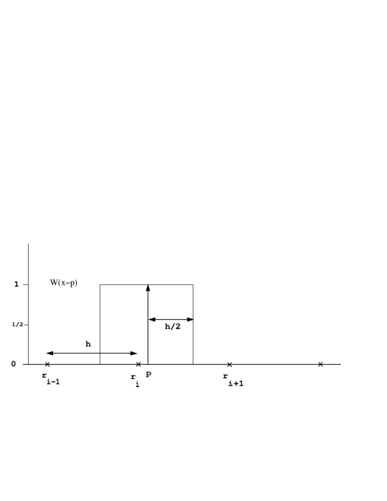
Figure 3.1: Kernel for the first order interpolation (NGP).

where $x_{p}$ is the position of the particle and $h$ is the mesh spacing of the grid on which we solve the field equations.

Figure 3.1 displays a typical NGP kernel operator for a particle at position $p$, and a grid with grid points at $r=r_{i-1}$, $r_{i}$, $r_{i+1}$, etc. This kernel will produce a density distribution given by:

$$\rho(x)=\sum_{i=1}^{N}\rho_{p}\ W(x-x_{p})$$ (3.21)

A commonly used higher order interpolation is called “cloud in cell” (CIC) interpolation which distributes the density of each particle into two grid cells. In this case the resulting density is piecewise linear and the kernel takes the form:

$$W(x-x_{p})=\left\{\begin{array}[]{r@{\quad:\quad}l}1-|x-x_{p}|/h&|x-x_{p}|\leq h\\ 0&{\mathrm{otherwise}}\end{array}\right.$$ (3.22)

Figure 3.2: Kernel for the second order interpolation (CIC).

Figure 3.2 is a graph of the kernel of the CIC interpolation. In our calculations we have used the CIC interpolation operator.

To restrict the Christoffel symbols (and other geometric quantities) calculated on the mesh to the particles’ positions we use the same kernel in the following way:

$$F(x_{p})=\sum^{N_{r}}_{i=1}F(x_{i})W(x_{i}-x_{p})$$ (3.23)

where $x_{p}$ is the position of the particle, $x_{i}$ are the grid points, and $F$ is any of the coefficients that appear in the evolution equations. The coefficients $F$ are products and quotients of the metric coefficients and their derivatives. In order to calculate derivatives we use the following finite difference approximation on the mesh:

$$\left[q^{\prime}\right]_{i}=\left(q_{i+1}-q_{i-1}\right)/h+O(h^{2})$$ (3.24)

and then use equation (3.23) to find an approximate value of $q^{\prime}$ at the particle’s position.

3.5 Initial Set of particles.

To initialize the set of particles which we evolve, we specify the particle distribution (number of particles per unit of areal coordinate) and the velocity distribution (specifically the number of particles per $p_{r}$ and $l$). This correspond to a distribution function in the sense of (2.1) which is separable in the $r$, $p_{r}$ and $l$ variables. In other words:

$$f(r,p_{r},l)=R(r)\,P(p_{r})\,L(l)$$ (3.25)

Moreover, instead of specifying $P$ as a function of $p_{r}$ we specify $P=P(\bar{p}_{r})$ where $\bar{p}_{r}=p_{r}/a$. This allow us to calculate the value of $p^{t}=\sqrt{m^{2}+\bar{p}_{r}^{2}+l^{2}/r^{2}}$, and therefore $\bar{\rho}$, $\bar{\j}_{r}$ and $\bar{S}$, for each particle without knowing the geometry in advance. This allows us to decouple the tasks of specify initial data for the particles, and ensuring that the initial data satisfies the constraint equations.

We use 1-dimensional Monte Carlo techniques applied to each of the functions $R(r)$, $P(p_{r})$, $L(l)$ to get an specific ensemble of the particles. In theory the statistical error that we produce goes like $O(N^{-1/2})$, where $N$ is the number of particles that we use to sample the distribution function (see section 4.3).

Chapter 4 Checks

In this chapter we explain different checks we have performed to test that we have properly implemented the algorithm. The first of these test was checking if the quantity given by equation (2.88) was conserved in the flat spacetime case. In our code this value was conserved up to the tolerance of the LSODA integrator for initial data which was gaussian in both the radial and velocity distributions. We have also checked that a test particle moving in a fixed background follows the geodesic of the background, and that its energy is conserved.

The rest of the checks that we describe here are for the fully coupled problem. In section 4.1 we discuss the conservation of the mass aspect function at the outer boundary ($r=r_{\mathrm{m}ax}$). We also have simulated certain clusters of particles in circular motion known as Einstein clusters; results from these simulations are discussed in 4.2 in section 4.2. At the end of the chapter we study how the numerical errors scale with the number of particles we use to sample the distribution function $f$, and as well as with the mesh spacing $h$.

4.1 Mass Conservation

The value of the mass function given by equation (2.89) at infinity should be a conserved quantity if the spacetime is asymptotically flat (see for instance [19]). As an approximation to the value at infinity we can monitor the value at the maximum value of the radial coordinate, $M(t,r_{\mathrm{m}ax})$. This check will make sense as long as no matter leaves the range of integration (note that energy cannot escape in the form of radiation since that is forbidden in spherical symmetry). In Figure 4.1 we plot $M(t,r_{\mathrm{m}ax})$ for three different mesh scales ($N_{r}=64$, $N_{r}=128$ and $N_{r}=256$) and with a fixed number of particles, $N=10000$.

Figure 4.1: Value of $2M(t,r)/r$ at $r=r_{\mathrm{m}ax}$ as a function of time.

We observe that the value of $M$ is conserved until $t\approx 40$ which s the time when the particles begin to leave the range of integration. In the inset we see a detail of the function between $t=0$ and $t=40$ showing that the conservation is better than $1\%$ for $N_{r}=64$ and improves somewhat as we increase the number of grid points. Theoretically (and in the limit $N\to\infty$) we should observe that the variation of the value of mass should decrease linearly with the number of points, i.e. first order. Although the convergence test here is not as definitive as it tends to be for pure finite-difference methods, the inset of Fig. 4.1 provides fairly good evidence that our code’s mass conservation would converge linearly with $h$ in the continuum limit.

4.2 Einstein Clusters

Probably the strongest check of the reliability of our code is its ability to simulate clusters of particles that only have rotational motion (zero radial component of the 4-momentum). Let us calculate what initial conditions we must set in order to obtain such a cluster.

Assuming we know what the energy density of the cluster of particles is, let us calculate the velocity profiles required in order to produce a cluster in equilibrium. In the process of obtaining the velocity profiles, we will also find the geometry of the spacetime created by the cluster. The metric coefficient $a(r)$ can be calculated using equation (2.89). If the spacetime is static then $\beta(r)=0$ and the resulting equation is:

$$a(r)=\left(1-2\frac{M(r)}{r}\right)^{-1},$$ (4.1)

where we calculate $M(r)$ by integrating the density $\rho(r)$ over the radial coordinate,
$M(r)=\int 4\pi r^{2}\rho(r)dr$. To calculate the lapse function we can make use of the evolution equation for the extrinsic curvature (2.23), which in this case reduces to:

$$\left(\frac{\alpha r}{a}\right)^{\prime}=\alpha a-4\pi\alpha ar^{2}\rho.$$ (4.2)

After a little bit of manipulation this equation can be written as:

$$\frac{\alpha^{\prime}}{\alpha}=-\frac{1-a^{2}}{2r}=\frac{M(r)}{r^{2}}\frac{1}{\left(1-2M(r)/r\right)}.$$ (4.3)

We want to find the angular momentum $l(r)$ needed to get the particles rotating with zero radial component of the 4 momentum. Imposing that condition ($p_{r}=0$ and $\partial p_{r}/\partial t=0$) on the geodesic equation for $p_{r}$, equation (2.77), we obtain:

$$-\frac{\partial\alpha}{\partial r}\bar{p}^{t}+\frac{l^{2}\alpha}{r^{3}\bar{p}^{t}}=0$$ (4.4)

Taking into account that

$$\bar{p}^{t}=\sqrt{m^{2}+\frac{l^{2}}{r^{2}}}\ ,$$ (4.5)

and using equation (4.3), we find the equation for $l(r)$:

$$l^{2}(r)=m^{2}r^{2}\left(\frac{M(r)}{r}\right)\frac{1}{\left(1-3M(r)/r\right)}$$ (4.6)

This is the same expression as the angular momentum for a particle in circular orbit around a Schwarzschild black hole with mass $M(r)$ (see [26]). In Figure 4.2 we have plotted the areal coordinate for some particles in a cluster with gaussian energy density profile and total mass $M\approx 0.57$ as a function of time. Further we can see that the particles retain roughly the same radial coordinate for a time longer than $500M$ (2 complete orbits). Also, the motion appears to be stable since the particles oscillate radially with roughly constant amplitude (see inset).

Figure 4.2: Radial coordinates of 7 particles as a function of time for a static cluster with gaussian energy density profile.

We found that for clusters with gaussian energy densities and initial maximum $6M/r=1.01$, the cluster becomes unstable and formed a black hole, whereas for clusters with initial maximum $6M/r=0.97$ the cluster was stable. This result agrees with the result that Einstein clusters become unstable for $6M/r=1$ (see [9] and references therein).

We have also simulated distorted static clusters for which we specify $(1-\epsilon)$ times the angular momentum fixed by (4.6); this allows us to control the deviation from the ideal static case. We have observed results similar to the case just described where the perturbation is effectively introduced by the numerical approximation itself; i.e. our distorted clusters tend to be stable when

$$\max_{t,r}\left(6M(t,r)/r\right)<1.$$ (4.7)

4.3 Numerical Errors.

There are two principal sources of numerical errors in our code: 1) sampling of the initial distribution function with a finite number of particles (statistical error), and 2) approximation of the derivatives in the field equations by finite-difference operators (truncation error).

In the continuum limit — where the number of particles, $N$, approaches infinity, and the mesh spacing, $h$, goes to $0$ — we need to check that these numerical errors go to zero to establish that, in this limit, we are solving the continuum system of equations (Vlasov equation coupled with Einstein’s equations).

First let us study how the statistical error varies with the number of particles. We can estimate the statistical error in one function by subtracting the functions computed using two different initial sets of particles (two different sets, each sampled using a Monte Carlo method and the same distribution function). Here, the specific function which we monitor is $2M(t,r)/r$, and we take the $L_{2}$ norm of the difference to be an estimate of the statistical error at each time. In other words, if ${}^{(1)}\left(2M(t,r)/r\right)$ and ${}^{(2)}\left(2M(t,r)/r\right)$ are calculated from two different sets of particles (generated from the same distribution function), then the statistical error estimate at a given time $t_{o}$ is computed by:

$$\Delta s(t_{o},r)={}^{(1)}\left(2M(t_{o},r)/r\right)-{}^{(2)}\left(2M(t_{o},r)/r\right).$$ (4.8)

Furthermore, we take the $L_{2}$ norm of this function:

$$\Delta s(t_{o})=\sqrt{\sum_{i=1}^{N_{r}}\Delta s(t_{o},r_{i})^{2}/N_{r}}$$ (4.9)

Figure 4.3: Statistical Error.

In Figure 4.3 we have plotted these estimates as a function of the number of particles at the initial time $t_{o}=0$ and for fixed mesh spacing, h. We have displayed 9 different estimates for the statistical error, and the shaded area of the graph shows bounds for the ensemble. The average slope is $m=-0.44\pm 0.08$ where the uncertainty is the standard deviation calculated from the individual slopes. We see that these results roughly agree with the expectation that the statistical error should scale as $N^{-1/2}$.

Figure 4.4: Truncation (dotted lines) and statistical error estimates (dashed lines) at t=0.

Let us turn our attention now to the truncation error. We assume a Richardson expansion for a mesh function $q^{h}(t,r)$, calculated with a given mesh spacing $h$:

$$q^{h}(t,r)=q(t,r)+\Delta q_{s}(t,r)+h^{p}e_{p}(t,r)+O(h^{p+1})$$ (4.10)

where $\Delta q_{s}$ is the statistical error. We estimate the truncation error in $q^{h}(t,r)$ via

$$q^{h}(t,r)-q^{h^{\prime}}(t,r)$$ (4.11)

where $h^{\prime}<h$, specifically we have used log$(h^{\prime})\approx-2.4$). In this way we use the function calculated with $h^{\prime}$ as a better approximation (a reference) to the analytic solution than the one with larger $h$. It is important that the statistical error $\Delta q_{s}\ll h^{p}e_{p}$ otherwise this recipe to calculate the estimate for the truncation error is meaningless since $q^{h}(t,r)-q^{h^{\prime}}(t,r)$ would be dominated by the statistical error.

In Figure 4.4 we show the base ten logarithm of the $L_{2}$ norm of the estimates of both the truncation and the statistical errors at $t=0$. We have plotted the truncation error estimates with dotted lines, and the statistical ones with dashed lines.

In these calculations we have not fixed the total number of particles, but rather the number of particles per grid cell (the value we use in this particular case is 500 particles per grid cell on average). The reason for fixing the number of particles per cell, rather than the total number of particles, is that the statistical error scales with $h$ (for the total number of particles fixed) roughly as $h^{-1}$. Increasing the number of particles as we decrease $h$, we compensate for this bias by maintaining roughly constant and small statistical error.

In the part of the Figure where the statistical error is much smaller than the truncation error we have calculated the average slope for the truncation error (the solid line in the Figure). The resulting slope is $m=2.02\pm 0.08$ where again the uncertainty is the standard deviation. At $t=0$ we thus observe second order convergence which is in agrement with the scheme that we have used to compute the geometric quantities.

Figure 4.5: Truncation (dotted lines) and statistical error estimates (dashed lines) at t=20.

Figure 4.5 shows the results of our error analysis at $t=20$. We see that in this case the slope is not $2$ but smaller, $m=1.36\pm 0.08$. This is consistent with the observation made in section 3.3 that the numerical scheme that we have used for the evolution is only first order accurate in $h$.

Chapter 5 Results

In this chapter we summarize the main results we have obtained. In order to find the critical solutions (solutions sitting at the threshold of black hole formation) we have performed bisection searches using the total rest mass (sum of the rest masses of the individual particles) of the cluster, $M_{o}$, as the search parameter $p$. In section 5.1 we discuss some characteristics of the critical solutions. In 5.2 we give some indications for the existence of a scaling laws, $\tau\sim-\sigma\ln{|p-p^{*}|}$, and we discuss the possibility of universality in the model in section 5.3. The chapter ends with some conclusions and some ideas for future work.

5.1 Is the critical solution Static ?

In this section we present evidence that, for initial data with non-zero angular momentum, as we approach criticality the solution for the space time approaches a static solution.

We will first focus on one family of initial conditions and afterwards we will try to explain what we observed for different families. The initial distributions on equation (3.25) are:

$$R(r) \propto r^{2}e^{\left(-(r-r_{o})^{2}/\Delta_{r}^{2}\right)}\,\Theta(r)$$ (5.1)

$$P(p_{r}) \propto e^{\left(-(\bar{p}_{r}-{\bar{p}_{r}}{}_{o})^{2}/{\Delta_{\bar{p}_{r}}}^{2}\right)}$$ (5.2)

$$L(l) \propto e^{\left(-(l-l_{o})^{2}/{\Delta_{l}}^{2}\right)}\,\Theta(l)$$ (5.3)

where $\bar{p}_{r}=p_{r}/a$, and $\Theta$ is the step or Heaviside function. For $r_{o}=5$, $\Delta_{r}=1$, $\bar{p_{r}}_{o}=0$, $\Delta_{\bar{p}_{r}}=2$, $l_{o}=12$, $\Delta_{l}=2$ (we will call this family “almost” time symmetric because the gaussian for the radial momentum is centered around $p_{r}=0$) we found the critical solution for a cluster rest mass about $M_{o}\approx 1.3$. In Figure 5.1 we show a few snapshots from the evolution of $da/dt$ resulting from initial data which is close to criticality but which eventually disperses. At early times, $da/dt$ oscillates, but between $t=117$ to $t=195$ it seems to get close to zero.

Figure 5.1: Snapshots of $da/dt$.

In the last snapshot ($t=234$) we observe how $da/dt$ has become negative, corresponding to dispersal of the particles. We observe similar behavior for the time derivatives of all the metric coefficients.

In order to see how close to zero $da/dt$ becomes, we show in Figure 5.2, a detail of $\dot{a}(t,r)$ at $t=156$ for three different sets of particles. The statistical error is roughly of the same order as the function itself (this is not true from $r\approx 6$ to $r\approx 8$ where the three ensembles agree on a non-zero value for the derivative, however we suspect that this feature will decrease if we tune closer to the critical solution and if we use greater resolution). This shows that the derivative of the function could be zero as we anticipate but it doesn’t give us a definite answer. The value of $da/dt$ could be smaller that the statistical error. In order to definitively answer this question we will need to have better resolution and decreased statistical errors.

Figure 5.2: Three ensembles of $da/dt$ at $t=156$.

As we have commented in section 2.4 an interesting function we monitor is $2M(t,r)/r$. This function is a scale invariant quantity which tells us a how close we are to trapped surface formation. We plot

$$\max_{r}\frac{2M(t,r)}{r}$$ (5.4)

in Figure 5.3. In the inset we show a detail for the period of time when the maximum seems to have a roughly constant value. Again, between $t=140$ and $t=190$ the statistical errors are of the same order as the fluctuations in $2M(t,r)/r$

Figure 5.3: $\max_{r}\left(2M(t,r)/r\right)$ as a function of time.

If we accept that the metric coefficients are independent of our time coordinate then we have a stationary space-time. If, in addition, the vector $N^{a}=d/dt$ introduced in Chapter (2) is orthogonal to the spatial hypersurfaces, then the space-time is static. This then implies that $\Omega_{a}=N_{a}$, or that the shift vector, and in particular the shift function $\beta(t,r)$, is zero.

In Figure 5.4 we show the evolution of the shift function. During the period when the time derivatives of the metric coefficients are close to zero, the shift function $\beta(t,r)$ also is close to zero, or at least of the same order as the statistical fluctuations as before. Thus the solution for the space-time sitting at the threshold of black hole formation could be a static solution (if it is not static, the amplitude of the derivatives and the shift function have small amplitudes relative to the statistical error).

Figure 5.4: Shift function as a function of time.

We also note that the total current density $j_{r}$ also tends to be of the order of the statistical fluctuations, but that the $S^{r}_{r}$ component of the stress energy tensor is not zero in the critical regime, as we can see in Figure 5.5. Therefore, on average there are the same number of particles with positive (outwards) and negative (inwards) $r$ components of the 4-momentum but the absolute value of $p_{r}$ is not zero on average.

This result and the fact that the maximum value of $2M(r)/r$ for this critical solution is $\sim 0.76$ indicate that this cannot be one of the Einstein clusters we have considered previously since there are no equilibrium clusters (either stable or unstable) with maximum $2M(r)/r$ larger than $2/3$.

Figure 5.5: Evolution of $\bar{S}_{r}(t,r)$.

5.2 Time Scaling

A Type I critical solution usually approaches a static or a periodic solution. As was argued in the previous section, we believe the critical solution in the current case is static. As we approach $p^{*}$ the dynamical solution spends more and more time close to this putative static solution.

We have calculated the time $t$ that each of the dynamical solutions spends inside some radius $r=r_{o}$ (in particular $r_{o}=6$). Figure 5.6 shows the plot of $\tau=t-t_{c}$ versus ln$(p)$ (natural logarithm) where $t$ is the time that the solution with search parameter $p$ spends inside $r=r_{o}$, and $t_{c}$ is the same quantity for the solution closest to criticallity.

We show three different ensembles of particles for the gaussian family given by equations (5.1-5.3) and again using “almost time symmetric” initial data.

Figure 5.6: Scaling law for the time. The error for each value of $\sigma$ is the standard deviation of the slope computed using a least squares fit.

We also have normalized the critical solution in such a way that it has ADM mass equal to $1$ at infinity, i.e.:

$$r \rightarrow r/M^{c}(t^{*},r_{\mathrm{m}ax})$$ (5.5)

$$t \rightarrow t/M^{c}(t^{*},r_{\mathrm{m}ax}),$$ (5.6)

where $M^{c}(t^{*},r_{\mathrm{m}ax})$ is the value of the mass aspect function at $r=r_{\mathrm{m}ax}$ for the solution closest to criticality during the critical regime. We can see that there is a rough linear relation between the time $\tau$ and ln$|p-p^{*}|$ with slope $-(5.2\pm 0.2)$ (the error is an estimate of the statistical error between different sets of particles):

$$\tau\sim-(5.2\pm 0.2)\ln|p-p^{*}|$$ (5.7)

Qualitatively this agrees with other type I critical solutions.

5.3 Different Families of Initial Data

The results we showed in the previous section are for Gaussian initial data given by equations [5.1- 5.3] with $p_{r}{}_{o}=0$ (“almost time symmetric” initial data) and $l_{o}=7$. In this section we show that similar results are found for other families of initial data. We have chosen initial data with $p_{r}{}_{o}=-4$ and $l_{o}=3$, $l_{o}=5$, $l_{o}=7$, $l_{o}=12$, (with same $r_{o}=5$, $\Delta_{r}=1$, $\Delta_{\bar{p}_{r}}=2$, $\Delta_{l}=2$ as before) and find that the critical solution for each of these cases appears to approach a static solution. For smaller values of the angular momentum the mass in the critical solution gets concentrated closer to the origin, which makes it more difficult to resolve the solution with a uniform finite-difference grid. We also have evolved an initial family with the following one particle distributions:

$$R(r) \propto \left(1-\tanh\left((r-r_{o})/\Delta_{r}\right)^{2}\right)\,\Theta(r)$$ (5.8)

$$P(p_{r}) \propto \left(1-\tanh\left((\bar{p}_{r}-{\bar{p}_{r}}{}_{o})/\Delta_{pr}\right)\right)$$ (5.9)

$$L(l) \propto \left(1-\tanh\left((l-l_{o})/\Delta_{l}\right)^{2}\right)\,\Theta(l)$$ (5.10)

with $r_{o}=5$,$\Delta_{r}=1$, ${\bar{p}_{r}}{}_{o}=-4$, $\Delta_{\bar{p}r}=2$, $l_{o}=7$, $\Delta_{l}=2$. For this distribution we also find that the solution with small $p-p^{*}$ ($p$ being the total rest mass of the cluster as before) spends some time close to an apparently static solution. In Figure 5.7 we show profiles for $2M(r)/r$ for the different families, each separate profile being selected from the corresponding period of near-critical evolution. Since different initial conditions set different scales for the problem we have normalized the results such that the total ADM mass of the solutions to which they approach is $1$ at infinity (rescaling given by equations (5.5-5.6)).

Figure 5.7: Critical solution for different families of initial data.

We can see that after normalization, the peak of $2M(r)/r$ is roughly at the same $r^{*}=2.3$. We can also see that the better a solution is resolved, the closer it conforms to the best resolved solution (the Gaussian with $l_{o}=7$ and “almost time symmetric” initial data). This is an indication that the critical solution might be universal although, we again need better resolution and more particles to be able to give a definitive answer.

We are also interested in seeing the importance of the distribution of angular momentum on the critical solutions. In Figure 5.8 we show $r^{2}\,\bar{S}^{a}{}_{a}(r)$ where $\bar{S}^{a}{}_{a}(r)$ is the function defined by equations (2.58) and (2.56) for the different families of initial data during the critical regime. This function, $r^{2}S^{a}{}_{a}(r)$, is a dimensionless quantity which measures the square of the angular momentum of the distribution of particles. We have rescaled the radial coordinate (and time) in the same way as in Figure 5.7.

Figure 5.8: $r^{2}\bar{S}^{a}{}_{a}(r)$ for the different families during the critical regime.

We can see that there is no apparent agreement between the functions calculated from different families of initial data. More work needs to be done in order to see what is the dependence of the critical solution with respect the angular momentum distribution. Moreover, estimates for the truncation and statistical errors for each calculation of the critical solutions must be calculated to properly compare the solutions.

Figure 5.9: Scaling behaviour for different families of initial data .

We have also estimated $\sigma$ defined by

$$\tau=-\sigma{\mathrm{l}n}|p-p^{*}|$$ (5.11)

for the different families. In Figure 5.9 we show the scaling behaviour for the different families of initial data that we have studied in this thesis. The error for each value of $\sigma$ in the Figure is, as beforre, the standard deviation of the slope computed using a least squares fit. We have collected the values that we have obtained for $\sigma$ in Table 5.1.

Family	$\sigma$
Gaussian,  $l_{o}=7$ (set 1)	$5.0\pm 0.2$
Gaussian, $l_{o}=7$ (set 2)	$5.0\pm 0.2$
Gaussian, $l_{o}=3$	$5.7\pm 0.2$
Gaussian, $l_{o}=5$	$5.5\pm 0.2$
Gaussian, $l_{o}=12$	$4.9\pm 0.2$
Gaussian, $l_{o}=12$ t.s. (set 1)	$5.1\pm 0.2$
Gaussian, $l_{o}=12$ t.s. (set 2)	$5.3\pm 0.2$
Gaussian, $l_{o}=12$ t.s. (set 3)	$5.2\pm 0.2$
Tanh, $l_{o}=7$	$5.9\pm 0.2$

Table 5.1: Values of time scaling exponent for the different families (t.s. stands for ”almost time symmetric”). The errors above are assumed to be the same as the statistical error for the t.s. family (see equation (5.7)).

5.4 Conclusions and Future Work

We have studied critical behavior at the threshold of black hole formation for collisionless matter. Our results indicate that, for families with non-zero angular momentua, the critical solution could be static with non-zero radial particle momenta. We have found evidence for a life-time scaling law which is to be expected for Type I critical solutions. In order to answer all these questions more rigorously we would need some way to increase our resolution where it is needed. Some kind of adaptive code (such as the ones used in finite difference studies [1]) would be useful.

It may be that the development of a finite difference code to solve the Vlasov equation directly in phase space would be the best way to attack this problem. This would allow us to incorporate the adaptivity that we need, as well as providing us with better-understood convergence properties.

Chapter A Summary of Equations in Maximal-Areal Coordinates

A.1 Field equations

$$\frac{a^{\prime}}{a} = \frac{1-a^{2}}{2r}+\frac{3}{2}ra^{2}{K^{\theta}_{\theta}}^{2}+4\pi ar\bar{\rho}$$ (A.1)

$${K^{\theta}_{\theta}}^{\prime} = -\frac{3}{r}K^{\theta}_{\theta}-4\pi\frac{\bar{j}_{r}}{a}$$ (A.2)

$$\alpha^{\prime\prime} = \alpha^{\prime}(\frac{a^{\prime}}{a}-\frac{2}{r})+\frac{2\alpha}{r^{2}}(a^{2}-1+2r\frac{a^{\prime}}{a})+4\pi a\alpha(\frac{\bar{S}^{r}_{r}}{a^{2}}+\bar{S}^{\theta}_{\theta}-3\bar{\rho})$$ (A.3)

$$\beta = \alpha rK^{\theta}_{\theta}$$ (A.4)

where

$$\bar{\rho} = \frac{1}{4\pi\Delta r}\sum_{i=1}^{N}\frac{\bar{p}^{t}_{i}}{r^{2}_{i}}W(r-r_{i})$$ (A.5)

$$\bar{S}^{r}_{r} = \frac{1}{4\pi\Delta r}\sum_{i=1}^{N}\frac{{{p_{r}}_{i}}^{2}}{\bar{p}^{t}_{i}r^{2}_{i}}W(r-r_{i})$$ (A.6)

$$\bar{S}^{\theta}_{\theta} = \frac{1}{4\pi\Delta r}\sum_{i=1}^{N}\frac{l^{2}_{i}}{r^{4}_{i}\bar{p}^{t}_{i}}W(r-r_{i})$$ (A.7)

$$\bar{\j}_{r} = \frac{1}{4\pi\Delta r}\sum_{i=1}^{N}\frac{{p_{r}}_{i}}{r^{2}_{i}}W(r-r_{i})$$ (A.8)

and

$$W(x-x_{i})=\left\{\begin{array}[]{r@{\quad:\quad}l}1-|x-x_{i}|/h&|x-x_{i}|\leq h\\ 0&{\mathrm{o}therwise}\end{array}\right.$$ (A.9)

A.2 Evolution Equations

$$\frac{dp_{r}}{dt} = -\frac{\partial\alpha}{\partial r}\bar{p}^{t}+\frac{\partial\beta}{\partial r}p_{r}+\frac{\alpha}{a^{3}}\frac{\partial a}{\partial r}\frac{{p_{r}}^{2}}{\bar{p}^{t}}+\frac{l^{2}\alpha}{\bar{p}^{t}r^{3}}$$ (A.10)

$$\frac{dr}{dt} = \frac{\alpha p_{r}}{a^{2}\bar{p}^{t}}-\beta$$ (A.11)

$$\bar{p}^{t} = \sqrt{m^{2}+\frac{{p_{r}}^{2}}{a^{2}}+\frac{l^{2}}{r^{2}}}$$ (A.12)

$$\frac{dp^{\theta}}{dt} = -\frac{2}{r}\left(\frac{\alpha p_{r}}{a^{2}\bar{p}^{t}}-\beta\right)p^{\theta}+\frac{1}{\tan{\theta}}\frac{\alpha}{\bar{p}^{t}}\left(\frac{l^{2}}{r^{4}}-{p^{\theta}}^{2}\right)$$ (A.13)

$$\frac{d\theta}{dt} = \frac{\alpha p^{\theta}}{\bar{p}^{t}}$$ (A.14)

$${p^{\phi}}^{2} = \frac{1}{\sin^{2}{\theta}}\left(\frac{l^{2}}{r^{4}}-{p^{\theta}}^{2}\right)$$ (A.15)

$$\frac{d\phi}{dt} = \frac{\alpha p^{\phi}}{\bar{p}^{t}}$$ (A.16)

Chapter B Direct Approach To Solutions of Einstein-Vlasov System

B.1 Field Equations

The distribution function is defined by:

$$f(t,r,p^{r},l)=\frac{dN}{dV},$$ (B.1)

where $N$ is the number of particles and $V$ is the volume in phase space. Then the stress energy tensor can be calculated via:

$$T^{\mu\nu}=\int\,p^{\mu}\,p^{\nu}\,f(t,r,p^{r},l)\,\frac{1}{m}\,dV_{p}$$ (B.2)

where the volume element in momentum space, $V_{p}$, is restricted by

$$-m^{2}=g_{\alpha\beta}\,p^{\alpha}\,p^{\beta}$$ (B.3)

to the following expression (see [13]):

$$dV_{p}=m\frac{dp_{r}\,dp_{\theta}\,dp_{\phi}}{p^{t}\,\sqrt{-g}}$$ (B.4)

We can introduce momentum coordinates adapted to the symmetry:

$$l^{2} = p_{\theta}^{2}+\frac{p_{\phi}^{2}}{\sin^{2}{\theta}}$$ (B.5)

$$\psi = \tan^{-1}{\frac{p_{\theta}\sin{\theta}}{p_{\phi}}}$$ (B.6)

and $\bar{p}^{t}$ given, as before, by:

$$\bar{p}^{t}=\sqrt{m^{2}+\frac{p_{r}^{2}}{a^{2}}+\frac{l^{2}}{r^{2}}}$$ (B.7)

The volume element $dV_{p}$ in these variables is:

$$dV_{p}=m\frac{dp_{r}dl^{2}d\psi}{2ar^{2}\bar{p}^{t}}$$ (B.8)

The stress-energy tensor components are:

$$T^{t}_{t} = \frac{-\pi}{a^{2}r^{2}}\int\bar{p}^{t}fdp_{r}dl^{2}+\frac{\beta\pi}{\alpha a^{2}r^{2}}\int p_{r}fdp_{r}dl^{2}$$ (B.9)

$$T^{t}_{r} = \frac{\pi}{a^{2}r^{2}\alpha}\int p_{r}fdp_{r}dl^{2}$$ (B.10)

$$T^{r}_{r} = \frac{-\beta\pi}{\alpha a^{2}r^{2}}\int p_{r}fdp_{r}dl^{2}+\frac{\pi}{a^{4}r^{2}}\int\frac{{p_{r}}^{2}}{\bar{p}^{t}}fdp_{r}dl^{2}$$ (B.11)

$$T^{\theta}_{\theta}=T^{\phi}_{\phi} = \frac{1}{2}\frac{\pi}{a^{2}r^{4}}\int\frac{l^{2}}{\bar{p}^{t}}dp_{r}dl^{2}$$ (B.12)

We are able then to construct the source terms:

$$\rho = \frac{\pi}{ar^{2}}\int{f(t,r,p_{r},l)\sqrt{m^{2}+\frac{p_{r}^{2}}{a^{2}}+\frac{l^{2}}{r^{2}}}dp_{r}dl^{2}}$$ (B.13)

$$j_{r} = \frac{\pi}{ar^{2}}\int{f(t,r,p_{r},l)p_{r}dp_{r}dl^{2}}$$ (B.14)

$$S^{r}_{r} = \frac{\pi}{a^{3}r^{2}}\int{\frac{p_{r}^{2}f(t,r,p_{r},l)}{\sqrt{m^{2}+p_{r}^{2}/a^{2}+l^{2}/r^{2}}}dp_{r}dl^{2}}$$ (B.15)

$$S^{\theta}_{\theta} = \frac{\pi}{ar^{4}}\int\frac{l^{2}f(t,r,p_{r},l)}{\sqrt{m^{2}+p_{r}^{2}/a^{2}+l^{2}/r^{2}}}dl^{2}dp_{r}$$ (B.16)

B.2 Vlasov Equation

If the system is collisionless, we have Liouville’s theorem concerning the conservation of the volume in phase space, $V$, and we also know that the particle number $N$ is a conserved quantity. Therefore we can write the conservation of the distribution function, $f=N/V$, as:

$$\frac{df}{d\tau}=0$$ (B.17)

This equation is known as the “collisionless Boltzmann’s equation” or the “kinetic equation”. Expanding the total derivative we have:

$$\frac{\partial x^{\alpha}}{\partial\tau}\frac{\partial f}{\partial x^{\alpha}}+\\ \frac{\partial p_{\alpha}}{\partial\tau}\frac{\partial f}{\partial p_{\alpha}}=0$$ (B.18)

where $x^{\alpha}$ are the space-time variables, and $p^{\alpha}$ are the momentum variables. In spherical symmetry this equation reduces to:

$$\frac{\partial f}{\partial t}+\\ \frac{\partial r}{\partial t}\frac{\partial f}{\partial r}+\\ \frac{\partial p_{r}}{\partial t}\frac{\partial f}{\partial p_{r}}=0$$ (B.19)

where $\partial r/\partial t$ and $\partial p_{r}/\partial t$ are given by equations (2.77) and (2.78). This gives:

$$\frac{\partial f}{\partial t}+\\ (\frac{\alpha p_{r}}{a^{2}\bar{p}^{t}}-\beta)\frac{\partial f}{\partial r}+\\ (-\frac{\partial\alpha}{\partial r}\bar{p}^{t}+\frac{\partial\beta}{\partial r}p_{r}+\frac{\alpha}{a^{3}}\frac{\partial a}{\partial r}\frac{{p_{r}}^{2}}{\bar{p}^{t}}+\frac{\alpha l^{2}}{\bar{p}^{t}r^{3}})\frac{\partial f}{\partial p_{r}}=0$$ (B.20)

Chapter C Summary of Equations in Polar-Areal Gauge Coordinates

In this section we present the equations for a second choice of coordinates. Specifically we again adopt areal radial coordinates (implying that the proper surface area of the spheres centered at $r=0$ and with radius $r$ will be $4\pi r^{2}$), but fix the time coordinate using polar slicing. This slicing condition is implemented by demanding:

$${\mathrm{T}r}K\equiv K^{i}{}_{i}=K^{r}{}_{r}$$ (C.1)

which implies $K^{\theta}{}_{\theta}=K^{\phi}{}_{\phi}=\dot{K}^{\theta}{}_{\theta}=\dot{K}^{\phi}{}_{\phi}=0$. Using expression (2.39) we can express $K^{\theta}{}_{\theta}$ as:

$$K^{\theta}{}_{\theta}=\frac{1}{rb\alpha}(\beta(rb)^{\prime}-r\dot{b})=0,$$ (C.2)

we have:

$$\beta(rb)^{\prime}=r\dot{b}$$ (C.3)

Choosing areal coordinates, $b=1$, $\dot{b}=0$, the above equation implies:

$$\beta=0.$$ (C.4)

The resulting metric is:

$$ds^{2}=-\alpha^{2}(t,r)dt^{2}+a^{2}(t,r)dr^{2}+r^{2}d\Omega$$ (C.5)

we then have the following geometrical quantities:

$$\begin{array}[]{c}R=2\left[-2\left(1/a\right)^{\prime}+a/r\left(1-1/a^{2}\right)\right]/(ar)\\ \\ \begin{array}[]{ll}R^{r}{}_{r}=2a^{\prime}/\left(ra^{3}\right)&R^{\theta}{}_{\theta}=R^{\phi}{}_{\phi}=1/\left(ar^{2}\right)\left(a-\left(r/a\right)^{\prime}\right)\\ \\ K^{r}{}_{r}=K=-\dot{a}/\left(a\alpha\right)&K^{\theta}{}_{\theta}=K^{\phi}{}_{\phi}=0\\ \\ {K^{i}}{}_{r|i}=-\left(\dot{a}/\left(a\alpha\right)\right)^{\prime}-2\dot{a}/\left(ra\alpha\right)&K_{|r}={K^{r}{}_{r}}_{,r}=-\left(\dot{a}/\left(a\alpha\right)\right)\\ \\ {\alpha_{|r}}^{|r}=1/a\left(\alpha^{\prime}/a\right)^{\prime}&{\alpha_{|\theta}}^{|\theta}={\alpha_{|\phi}}^{|\phi}=\alpha^{\prime}/\left(a^{2}r\right)\end{array}\end{array}$$ (C.6)

Briefly we summarize the resulting equations of motion:

Momentum Constraint:

$$\dot{a}=-4\pi ra\alpha j_{r}$$ (C.7)

Hamiltonian Constraint:

$$a^{\prime}=4\pi ra^{3}\rho-\frac{a}{2r}(a^{2}-1)$$ (C.8)

Evolution of the 3-metric

$$\dot{g}_{ij}=-2\alpha g_{ik}K^{k}_{j}$$ (C.9)

Evolution of the extrinsic curvature

$$\dot{K}^{r}{}_{r} = -\frac{1}{a}\left(\frac{\alpha^{\prime}}{a}\right)^{\prime}+\frac{2\alpha a^{\prime}}{ra^{4}}+4\pi\alpha(S-\rho)-8\pi\alpha S^{r}{}_{r}$$ (C.10)

$$\dot{K}^{\theta}{}_{\theta} = 0=-\frac{\alpha^{\prime}}{a^{2}r}+\frac{\alpha}{ar^{2}}\left(a-\frac{1}{a}+r\frac{a^{\prime}}{a^{2}}\right)+4\pi\alpha(S-\rho)-8\pi\alpha S^{\theta}{}_{\theta}$$ (C.11)

$$\dot{K}^{\phi}{}_{\phi} = 0=-\frac{\alpha^{\prime}}{a^{2}r}+\frac{\alpha}{ar^{2}}\left(a-\frac{1}{a}+r\frac{a^{\prime}}{a^{2}}\right)+4\pi\alpha(S-\rho)-8\pi\alpha S^{\phi}{}_{\phi}$$ (C.12)

where the two last equations are zero by the choice of slicing.

Chapter D Pseudo-code

Ignacio (Iñaki) Olabarrieta

routine vlasov
  # $r_{i}$ := position of the i-th particle
  # $[p_{\mu}]_{i}$ := momentum of i-th the particle
  # $[T^{\mu}_{\nu}]_{j}$ := $T^{\mu}_{\nu}$ component on the j grid point
  # $a_{j}$, $\alpha_{j}$ and $\beta_{j}$ are the metric coefficients
  # $M_{j}$ := mass aspect function
  # Generate the initial positions $r_{i}$ and velocities $[p_{\mu}]_{i}$ for the particles
  read parameters of the distribution function
  for $i=1...N_{particles}$
      Generate $r_{i}$ and $[p_{\mu}]_{i}$ using Monte Carlo for a given distribution function
  end for
  t = 0
  # Time loop
  while $t<t_{max}$
        for $j=1...N_{gridpoints}$
            Calculate $[T^{\mu}_{\nu}]_{j}$ from $r_{i}$ and $[p_{\mu}]_{i}$
        end for
        Solve for $a_{j}$, $\beta_{j}$ and $\alpha_{j}$ on the mesh
        # Check apparent horizon formation
        if $2M_{j}/r_{j}=1$  stop
        Ouput $a_{j}$, $\beta_{j}$ and $\alpha_{j}$
        for $i=1...N_{particles}$
            Calculate $[\Gamma^{\mu}_{\nu\eta}]_{i}$ at $t=t+1/2\ dt$ from $a_{j}$, $\beta_{j}$ and $\alpha_{j}$
        end for
        t = t + dt
        for $i=1...N_{particles}$
            Integrate geodesic equations to find new $r_{i}$ and $[p_{\mu}]_{i}$
            if $r_{i}>r_{max}$ Kill i-th particle, $N_{particles}=N_{particles}-1$
            if $r_{i}<0$    Reflect the particle
            if $N_{particles}=0$    stop
        end for
  end while
end routine

References

- [1] M.W. Choptuik, “Universality and scaling in the gravitational collapse of a scalar field”. Phys. Rev. Lett., 70, 9-12, 1993.
- [2] M.W. Choptuik, P.Bizon, and T. Chmaj, “Critical Behaviour in Gravitational Collapse of a Yang-Mills Field”. Phys. Rev. Lett., 77, 424-427, 1996
- [3] C. Gundlach, “Critical phenomena in gravitational collapse”. Adv. Theor. Math. Phys. 2 (1998) 1 [gr-qc/9712084].
- [4] A. Einstein, “On Stationary System with Spherical Symmetry Consisting of Many Gravitating Masses”. Ann. Math., 40, 922-936, 1939
- [5] J.R. Oppemheimer and H. Snyder, “On Continued Gravitational Contraction”. Phys. Rev., 56, 455-459, 1939
-
[6]
R.C. Tolman,
“Effect of Inhomogeneity on Cosmological Models”.
Proc. Nat. Acad. Sci., 20, 169-176, 1934 - [7] H. Bondi, “Spherically Symmetrical Models in General Relativity”. Mon. Not. Roy. Astr. Soc., 107, 410-425, 1947
- [8] D.M. Eardley, “Time functions in numerical relativity: Marginally bound dust collapse”. Phys. Rev. D, 19, 2239-2259, 1979
- [9] S.L. Shapiro and S. Teukolsky, “Relativistic Stellar Dynamics on the Computer. I. Motivation and Numerical Method”. Ap. J., 298, 34-57, 1985
- [10] S.L. Shapiro and S. Teukolsky, “Relativistic Stellar Dynamics on the Computer. II. Applications”. Ap. J., 298, 58-79, 1985
- [11] S.L. Shapiro and S. Teukolsky, “The Collapse of Dense Star Clusters to Supermassive Black Holes: The Origin of Quasars and AGNs”. Ap. J., 292L, 41-44, 1985
- [12] S.L. Shapiro and S. Teukolsky, “Relativistic Stellar Dynamics on the Computer. IV. Collapse of a Star Cluster to a Black Hole”. Ap. J., 307, 575-592, 1986
- [13] F.A. Rasio, S.L. Shapiro, S.A. Teukolsky, “Solving The Vlasov Equation in General Relativity”. Ap. J., 344, 146-157, 1989
- [14] S.L. Shapiro, S.A. Teukolsky, “Formation of Naked singularities: The violation of Cosmic Censorship”. Phys. Rev. Lett., 66, 994-997, 1991
- [15] G. Rein, “Static solutions of the spherically symmetric Vlasov-Einstein system”. (unpublished) [gr-qc/9304028].
- [16] G. Rein, A.D. Rendall, “Global existence of classical solutions to the Vlasov-Poisson system in a three-dimensional, cosmological setting”. (unpublished) [gr-qc/9306021].
- [17] A.D. Rendall, “An introduction to the Einstein-Vlasov system”. (unpublished) [gr-qc/9604001].
- [18] G. Rein, A.D. Rendall and J. Schaeffer, “Critical collapse of collisionless matter: A numerical investigation”. Phys. Rev. D58 (1998) 044007 [gr-qc/9804040].
- [19] C.W. Misner, K.S. Thorne, J.A. Wheeler, “Gravitation”. W.H. Freeman, San Francisco, 1973
-
[20]
M.W. Choptuik,
“The 3+1 Einstein Equations”, (unpublished notes), 1998
http://laplace.physics.ubc.ca/People/matt/Teaching/98Spring/
Phy387N/Notes.html - [21] R.W. Hockney, J.W. Eastwood, “Computer Simulation Using Particles”. McGraw-Hill Inc.,1981
- [22] L.R. Petzold and A.C. Hindmarsh, “LSODA”. Computing and Mathematics Research Division, l-316 Lawrence Livermore National Laboratory, Livermore, CA 94550.
-
[23]
E. Anderson et al,
“LAPACK Users’ Guide”.
Society for Industrial and Applied Mathematics, Philadelphia, 1992
[http://www.netlib.org/lapack/lug/lapack_lug.html] - [24] J. W. York, “Kinematics and Dynamics of General Relativity”, in “Sources of Gravitational Radiation”, L. Smarr, ed. Cambridge University Press, 1979
- [25] M.W. Choptuik, “Numerical Techniques for Radiative Problems in General Relativity”. Univ. of British Columbia Ph.D. thesis (unpublished), 1986
- [26] R.M. Wald, “General Relativity”. The University of Chicago Press, 1984