Numerical Investigation of Cosmological Singularities

Abstract

A primary unresolved issue for cosmological singularities is whether or not their behavior is locally of the Mixmaster type (as conjectured by Belinskii, Khalatnikov, and Lifshitz (BKL)). The Mixmaster dynamics first appears in spatially homogeneous cosmologies of Bianchi Types VIII and IX. A multiple of the spatial scalar curvature acts as a closed potential leading, in the evolution toward the singularity (say $\tau\to\infty$), to an (almost certainly) infinite sequence of bounces whose parameters exhibit the sensitivity to initial conditions usually associated with chaos. Other homogeneous cosmologies are characterized by open (or no) potentials leading to a last bounce as $\tau\to\infty$ . Such models are called asymptotically velocity term dominated (AVTD). Here we shall describe a numerical approach to address the BKL conjecture. Starting with a symplectic numerical method ideally suited to this problem, we shall consider application of the method to three models of increasing complexity. The first application is to spatially homogeneous (vacuum) Mixmaster cosmologies where we compare the symplectic ODE solver to a Runge-Kutta one. The second application is to the (plane symmetric, vacuum) Gowdy universe on $T^{3}\times R$. The dynamical degrees of freedom satisfy nonlinearly coupled PDE’s in one spatial dimension and time. We demonstrate support for conjectured AVTD behavior for this model and explain its observed nonlinear small scale spatial structure. Finally, we study $U(1)$ symmetric, vacuum cosmologies on $T^{3}\times R$. These are the simplest spatially inhomogeneous universes in which local Mixmaster dynamics is allowed. The Gowdy code is easily generalized to this model, although, the spatial differencing needed in the symplectic method is not trivial.For AVTD models, we expect the potential-like term in the Hamiltonian constraint to vanish as $\tau\to\infty$ while in local Mixmaster it becomes (locally) large from time to time. We show how the potential behaves for a variety of generic $U(1)$ models.

1 Introduction

In these lectures, I propose to discuss the application of symplectic numerical methods [1, 2] to the investigation of cosmological singularities. For a system whose evolution can be described by a Hamiltonian, the symplectic approach splits the Hamiltonian into kinetic and potential subhamiltonians. If the subhamiltonians are exactly solvable, these solutions can be used to evolve the system from one time to the next. Fortunately, an appropriate choice of variables in the standard $3+1$ Hamiltonian formulation of general relativity enables Einstein’s equations to be derived from a Hamiltonian appropriate for the symplectic algorithm (SA). So far, the primary application of SA to general relativity has been to determine the asymptotic singularity behavior of cosmological models (but see also [3]). The SA is well-suited to this problem because it becomes exact if the asymptotic behavior is asymptotically velocity term dominated (AVTD)—i.e. the kinetic subhamiltonian asymptotically determines the dynamics.

To study the application of SA to general relativity, we shall consider a sequence of models whose variables depend on 0, 1, and 2 spatial dimensions. The first case we shall consider is the spatially homogeneous Mixmaster universe. (For convenience, we shall consider only the diagonal Bianchi IX vacuum model.) Einstein’s equations can be obtained by variation of the Hamitonian

$$2{\cal H}=-p_{\Omega}^{2}+p_{+}^{2}+p_{-}^{2}+U(\Omega,\beta_{+},\beta_{-})$$ (1)

where

$$U = e^{4\Omega}\left({e^{-8\beta_{+}}+e^{4(\beta_{+}+\sqrt{3}\beta_{-})}+e^{4(\beta_{+}-\sqrt{3}\beta_{-})}}\right.$$ (2)

$$\quad\quad\quad\quad\left.{-2e^{4\beta_{+}}-2e^{-2(\beta_{+}+\sqrt{3}\beta_{-})}-2e^{-2(\beta_{+}-\sqrt{3}\beta_{-})}}\right).$$

Here $\Omega(t)$ is the logarithm of the cosmological scale factor and measures isotropic expansion, while $\beta_{\pm}$ measure orthogonal anisotropic shears with $p_{\Omega}$ and $p_{\pm}$ respectively canonically conjugate to $\Omega$ and $\beta_{\pm}$ [4]. The potential $U$ is proportional to the spatial scalar curvature ($U=e^{6\Omega}\ {}^{3}\/\/R$) and is shown in Fig. 1.

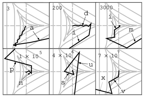
Figure 1: A typical Mixmaster trajectory in the anisotropy plane with horizontal axis $\beta_{+}$ and vertical axis $\beta_{-}$ which are centered on zero. Time increases (and the singularity is approached) to the right and downward. The number on each frame indicates the axes’ scales. The letters label the Kasner epochs. The Mixmaster minisuperspace equipotentials are shown shaded in gray.

Eq. (1) is itself the Hamiltonian constraint ${\cal H}=0$. The properties of this model have been known (more or less) since the late sixties [5, 6]. The first three terms in $U$ describe triangular walls. As the model evolves toward the singularity at $\Omega=\infty$, the walls become exponentially steep. Within the walls, the system behaves almost as a free particle ($U\approx 0$). In the approach to the singularity, $\Omega$ itself may be used as the time variable. As $\Omega\to-\infty$, a fixed value of $U$, say $U_{0}$, moves outward in the $\beta_{\pm}$-plane at a speed $1/2$ that of the system point [7]. Thus the system evolves with an infinite sequence of bounces off the potential. A typical trajectory is shown in Fig. 1. While there is no exact solution, each straight line segment can be parametrized and a map (the BKL map) derived to link one segment to the next [5, 8, 9]. There is a long history of numerical simulations [10], [11] trying to assess the validity of the BKL map as a descriptor of the dynamics. Part of this interest can be traced to the fact that a bounce which leaves one of the $120^{\circ}$ corners of the potential to move to another corner exhibits the sensitivity to initial conditions usually associated with chaos. Whether or not Mixmaster dynamics is chaotic remains a topic for both analytic and numerical study [11]. We note that with $U=0$, the solution is that of Kasner [12]. A solution which is asymptotically Kasner is AVTD. The Mixmaster solution is the antithesis of AVTD since there is (presumably) no last bounce. The effect of the spatial derivatives that generate $U$, though almost absent during each Kasner epoch, always recurs.

Our remaining examples are spatially inhomogeneous cosmologies (still vacuum for convenience). Long ago, BKL conjectured that the singularity in spatially inhomogeneous cosmologies is locally of the Mixmaster type [5]. Analytic verification of the BKL conjecture has bogged down on the issue of setting up the local Mixmaster behavior in a global way. For this reason, a numerical approach may be useful.

While our second model’s plane symmetry precludes local asymptotic Mixmaster dynamics, it does serve as an excellent laboratory for the SA. The Gowdy model on $T^{3}\times R$ is described by the metric [13]

$$ds^{2} = e^{{{-\lambda}\mathord{\left/{\vphantom{{-\lambda}2}}\right.\kern-1.2pt}2}}e^{{\tau\mathord{\left/{\vphantom{\tau 2}}\right.\kern-1.2pt}2}}(-\,e^{-2\tau}\,d\tau^{2}+d\theta^{2})$$ (3)

$$+e^{-\tau}\,[e^{P}d\sigma^{2}+2e^{P}Q\,d\sigma\,d\delta+(e^{P}Q^{2}+e^{-P})\,d\delta^{2}]$$

where $\lambda$, $P$, $Q$ are functions of $\theta$, $\tau$. We impose $T^{3}$ spatial topology by requiring $0\leq\theta,\sigma,\delta\leq 2\pi$ and the metric functions to be periodic in $\theta$. If we assume $P$ and $Q$ to be small, we find them to be respectively the amplitudes of the $+$ and $\times$ polarizations of the gravitational waves with $\lambda$ describing the background in which they propagate. The time variable $\tau$ measures the area in the symmetry plane with $\tau=\infty$ a curvature singularity. Einstein’s equations split into two groups. The first is nonlinearly coupled wave equations for $P$ and $Q$ (where $,_{a}=\partial/{\partial a}$):

$$P,_{\tau\tau}-\;e^{-\kern 1.0pt2\tau}P,_{\theta\theta}-e^{2P}\left({Q,_{\tau}^{2}-\;e^{-\kern 1.0pt2\tau}Q,_{\theta}^{2}}\right) = 0,$$ (4)

$$Q,_{\tau\tau}-\;e^{-\kern 1.0pt2\tau}Q,_{\theta\theta}+\,2\,\left({P,_{\tau}Q,_{\tau}-\;e^{-\kern 1.0pt2\tau}P,_{\theta}Q,_{\theta}}\right) = 0.$$ (5)

The second contains the Hamiltonian and $\theta$-momentum constraints which can be expressed as first order equations for $\lambda$ in terms of $P$ and $Q$:

$$\lambda,_{\tau}-\;[P,_{\tau}^{2}+\;e^{-2\tau}P,_{\theta}^{2}+\;e^{2P}(Q,_{\tau}^{2}+\;e^{-2\tau}\,Q,_{\theta}^{2})]=0,$$ (6)

$$\lambda,_{\theta}-\;2(P,_{\theta}P,_{\tau}+\;e^{2P}Q,_{\theta}Q,_{\tau})=0.$$ (7)

This break into dynamical and constraint equations removes two of the most problematical areas of numerical relativity from this model: (1) The normally difficult initial value problem becomes trivial since $P$, $Q$ and their first time derivatives may be specified arbitrarily (as long as the total $\theta$ momentum in the waves vanishes). (2) The constraints, while guaranteed to be preserved in an analytic evolution by the Bianchi identities, are not automatically preserved in a numerical evolution with Einstein’s equations in differenced form. However, in the Gowdy model, the constraints are trivial since $\lambda$ may be constructed from the numerically determined $P$ and $Q$. For the special case of the polarized Gowdy model ($Q=0$), $P$ satisfies a linear wave equation whose exact solution is well-known [14]. For this case, it has been proven that the singularity is AVTD [15]. This has also been conjectured to be true for generic Gowdy models [16]. We shall show in Section 4 how the SA applied to this model provides strong support for this conjecture.

Our final model generalizes the plane symmetry to a U(1) symmetry [17]. The details of this model will be given in Section 5. $U(1)$ models allow local Mixmaster dynamics and thus can be used to test the BKL conjecture. In fact, it is possible that any type of allowed cosmological singularity will already appear in the $U(1)$ models. The extension of the Gowdy SA methods to the $U(1)$ case is straightforward.

2 Symplectic Methods

Consider the time evolution of a set of variables $X$ from $t_{1}$ to $t_{2}$. We can define an evolution operator ${\cal U}(t_{2},t_{1})$ such that if f $t_{2}-t_{1}=\Delta t$ is infinitesimal, then ${\cal U}$ must have the form

$${\cal U}(\Delta t)X=\left(1+\Delta t\frac{d}{dt}\right)X.$$ (8)

But ${dX}/{dt}=\{H,X\}$ where $\left\{{H,X}\right\}$ is the Poisson bracket with $H$ the Hamiltonian. Thus ${\cal U}(\Delta t)=1+\Delta t\{H,\quad\}$ with the empty slot in the operator to act on $X$. In the standard way (by dividing $\Delta t$ into $n$ intervals and applying ${\cal U}({\Delta t}/n)$ $n$ times) we obtain the exponentiated form (for finite $\Delta t$)

$${\cal U}(\Delta t)=e^{\Delta t\{H,\quad\}}\equiv e^{\Delta tA}.$$ (9)

Suppose $H=H_{1}+H_{2}$. Then ${\cal U}=e^{\Delta t(A_{1}+A_{2})}$. Consider

$${\cal U}_{(2)}(\Delta t)=e^{A_{1}(\Delta t/2)}e^{A_{2}\Delta t}e^{A_{1}(\Delta t/2)}.$$ (10)

Straightforward multiplication shows that the right hand side of (10) is a second order accurate approximation to the evolution operator $e^{\Delta tA}$. One evolves $X$ from $t$ to $t+\Delta t$ by first evolving with $e^{{{(\Delta t}/2)}A_{1}}$ from $t$ to $t+\frac{1}{2}{\Delta t}$, taking that result and evolving with $e^{\Delta tA_{2}}$ from $t$ to $t+\Delta t$, and, finally, evolving that result with $e^{{{(\Delta t}/2)}A_{1}}$ from $t+\frac{1}{2}{\Delta t}$ to $t+\Delta t$.

Suzuki has shown how to obtain a representation of ${\cal U}$ to arbitrary order [18]. For example,

$${\cal U}_{(4)}(\Delta t)={\cal U}_{(2)}(s\Delta t){\cal U}_{(2)}[(1-2s)\Delta t]{\cal U}_{(2)}(s\Delta t)$$ (11)

where $s=(2-2^{1/3})^{-1}$. In general,

$${\cal U}_{(2m)}(\Delta t)={\cal U}_{(2m-2)}(s_{m}\Delta t){\cal U}_{(2m-2)}[(1-2s_{m})\Delta t]{\cal U}_{(2m-2)}(s_{m}\Delta t)$$ (12)

where $s_{m}=(2-2^{1/{(2m-1)}})^{-1}$. As a concrete example, consider the Hamiltonian

$$H=H_{1}+H_{2}={\textstyle{1\over 2}}p^{2}+V(q)$$ (13)

where $V$ is an arbitrary potential. Note that both $H_{1}$ and $H_{2}$ yield exact solutions. For $H_{1}$,

$$q(t+\Delta t) = q(t)+p(t)\Delta t,$$

$$p(t+\Delta t) = p(t),$$ (14)

while for $H_{2}$,

$$q(t+\Delta t) = q(t),$$

$$p(t+\Delta t) = p(t)-\left.\frac{dV}{dq}\right|_{t}\,\Delta t.$$ (15)

Since $q$ is constant for the Hamiltonian $H_{2}$, the solution for $p$ is exact no matter how complicated the potential $V$. Thus the exact solutions (2) and (2) are used to evolve from $t$ to $t+\Delta t$ according to the prescription ${\cal U}_{(2)}(\Delta t)$. To go to higher order, nothing new is required. The time intervals are selected according to the prescription (12), but the same exact solution is used.

Extension to fields $q(x,t)$, $p(x,t)$ is straightforward. With computation in mind, define $q_{i}^{j}\equiv q(x_{i},t^{j})$, etc. where $x_{i}=i\Delta x$ and $t^{j}=j\Delta t$. Then the exact solutions are for $H_{1}$

$$(q_{i}^{j+1},p_{i}^{j+1})=(q_{i}^{j}+p_{i}^{j}\Delta t,p_{i}^{j})$$ (16)

and for $H_{2}$

$$\left(q_{i}^{j+1},p_{i}^{j+1}\right)=\left(q_{i}^{j},p_{i}^{j}-\left.\frac{\delta V}{\delta q}\right|_{i}^{j}\Delta t\right)$$ (17)

where ${\delta V/\delta q}$ is the appropriate functional derivative. Again, the exact solution exists for $H_{2}$ no matter how complicated the potential. Of course, one must represent the spatial derivative ${\delta V/\delta q}$ as accurately as possible.

To represent spatial derivatives to the desired order, evaluate (e.g. in 1D) the Taylor series for an arbitrary function $f(x)$. Say the 4th order accurate expression for $d^{2}f/dx^{2}$ is desired. Demand that

$$a_{1}\left[{f(x+\varepsilon)+f(x-\varepsilon)}\right] + a_{2}\left[{f(x+2\varepsilon)+f(x-2\varepsilon)}\right]$$ (18)

$$= {{d^{2}f}\over{dx^{2}}}\varepsilon^{2}+O(\varepsilon^{6}).$$

We find $a_{1}=\frac{4}{3}$, $a_{2}=-\frac{1}{12}$. A similar procedure can be used for any term in the Taylor expansion. It can also be extended to two spatial dimensions where the same coefficients are found. Extension to higher order requires $f(x+n\varepsilon)$ for some $n>2$ (depending on order).

The only remaining issue in the evaluation of $({{{dV}\mathord{\left/{\vphantom{{dV}{dq}}}\right.\kern-1.2pt}{dq}}})_{i}^{j}$ is whether to vary $V$ analytically and then difference the variation or difference $V$ and then vary the differenced form. We have chosen the latter. (For complicated $V$, the two are equivalent only to some order.) As a simple example, again consider $d^{2}f/dx^{2}$ to arise from the variation of $V={1\over 2}\left({{{df}\over{dx}}}\right)^{2}$. Since the Hamiltonian for this case is $H_{2}=\int{V[q(x,t)]\kern 1.0pt\,dx}$, the differenced form is (for 2nd order accuracy)

$$H_{2}={1\over 2}\sum\limits_{i=1}^{N}{{{\left({f_{i+1}-f_{i}}\right)^{2}}\over{(\Delta x)^{2}}}}.$$ (19)

(The negative of) the variation with respect to $f_{i}$ (which appears in two terms of the sum) yields the standard differenced second derivative $(f_{i+1}+f_{i-1}-2f_{i})/(\Delta x)^{2}$.

3 Mixmaster Model

Although I have done several computational projects with the Mixmaster model, (see references in [9, 20]), none of these have used the SA. Here we shall use Mixmaster primarily as an application of SA rather than to evaluate Mixmaster parameters or to compute Lyapunov exponents [19, 20]. The Hamiltonian (1) clearly is in the correct form with $H_{1}=-p_{\Omega}^{2}+p_{+}^{2}+p_{-}^{2}$ and $H_{2}=U(\beta_{\pm},\Omega)$ having obvious exact solutions.

(The variables chosen are not the only ones that have been used. For example, the ADM reduction can be performed by choosing $\Omega$ to be the time variable and solving the Hamiltonian constraint (1), ${\cal H}=0$, for $p_{\Omega}$. The remaining degrees of freedom for $\beta_{\pm}$ are dynamical. Since the constraint is automatically preserved, one might argue that this choice is better. However, the ability to monitor $H$ as an indicator of the accuracy and stability of the solution outweighs the disadvantage of the extra degree of freedom.)

There is actually some debate over the optimal choice of ODE solver (see e.g. [21]). The choice will involve trade-offs between accuracy and computer time. Accuracy is especially important for models with sensitivity to initial conditions since a small numerical error could qualitatively change the solution. (Sensitivity to initial conditions means that an arbitrarily small change in initial data can generate qualitatively different trajectories. Numerical error could simulate change in initial conditions.) Here we shall consider only comparisons between a 4th order Runge-Kutta algorithm (RKA) [22] and 4th and 6th order SA’s. In all cases, the same initial data set (freely specify $\Omega$, $\beta_{\pm}$, and $p_{\pm}$ and solve ${\cal H}=0$ for $p_{\Omega}$) is run for up to 2000 time steps. An adaptive step size algorithm has been borrowed from [22] for use in all these codes. A modification to limit the maximum step size is required to avoid seriously over-running a Mixmaster wall. When this eventually occurred anyway, the computation was stopped. Fig. 2 displays the results for the three codes at a single Mixmaster bounce.

Figure 2: Close up of a Mixmaster bounce in the anisotropy plane. The same input file was evolved with a 4th order RKA (open circles) and two SA’s of 4th (open triangles) and 6th (filled squares) order. The same adaptive step size subroutine was used in all cases.

Note that the 4th order SA and RKA have similar performance while the 6th order SA equally well represents the solution with many fewer time steps. The 6th order SA easily reached $\tau>10^{6}$, more than two orders of magnitude greater than RKA in essentially the same number of steps. The much larger time step possible with the 6th order SA easily overcomes tje extra computational time needed to take a 6th order step as three 4th order ones. It is only now that SA’s are being applied to the study of Mixmaster [23] and related models [3].

4 Gowdy Model on $T^{3}\times R$

The SA can be applied to the Gowdy cosmology because the wave equations (4) can be obtained by variation of the Hamiltonian

$$H = {1\over 2}\int\limits_{0}^{2\pi}{d\theta\,\left[{\pi_{P}^{2}+\kern 1.0pt\,e^{-2P}\pi_{Q}^{2}}\right]}$$ (20)

$$+ {1\over 2}\int\limits_{0}^{2\pi}{d\theta\,\left[{e^{-2\tau}\left({P,_{\theta}^{2}+\;e^{2P}Q,_{\theta}^{2}}\right)}\right]}=H_{1}+H_{2}.$$

Again equations obtained from the separate variations of $H_{1}$ and $H_{2}$ are exactly solvable. Variation of $H_{1}$ yields terms in (4) containing time derivatives. These have the exact (AVTD) solution

$$P = -\beta\tau+\ln[\alpha\,(1+\zeta^{2}e^{2\beta\tau})]\to\beta\tau\quad{\rm as}\ \tau\to\infty,$$ (21)

$$Q = -\;{{\zeta\,e^{2\beta\tau}}\over{\alpha\,(1+\zeta^{2}e^{2\beta\tau})}}+\xi\quad\to Q_{0}\ \;{\rm as}\ \tau\to\infty\ ,$$ (22)

$$\pi_{P} = {-{\beta(1-\zeta^{2}e^{2\beta\tau})}\over{(1-\zeta^{2}e^{2\beta\tau})}}\quad\to\beta\ \;{\rm as}\ \tau\to\infty\ ,$$ (23)

$$\pi_{Q} = -2\alpha\beta\zeta$$ (24)

in terms of four constants $\alpha$, $\beta$, $\zeta$, and $\xi$. To employ the AVTD solution in the SA, the values of $P$, $Q$, $\pi_{P}$, and $\pi_{Q}$ at $t^{j}$ are used to find $\alpha$, $\beta$, $\zeta$, and $\xi$. These are substuted in (21) to evolve to new values at $t^{j+1}$ according to (10). Note that evolution with $H_{1}$ is purely local since there are no spatial derivatives. This is advantageous for parallel processing.

Evolution with $H_{2}$ is still easy because $P$ and $Q$ are constant. The necessary differencing has already been discussed in Section 2. For completeness, we give the (2nd order) differenced form of $H_{2}$ as

$$H_{2}={{e^{-2\tau}}\over{(\Delta\theta)^{2}}}\sum\limits_{i=0}^{N}{{\left[{\left({P_{i}-P_{i-1}}\right)^{2.}+e^{P_{i}+P_{i-1}}\left({Q_{i}-Q_{i-1}}\right)^{2}}\right]}.}$$ (25)

The presence of only points and nearest neighbors in (25) also yields easy parallelization. The exponential prefactor $e^{-2\tau}$ in $H_{2}$ makes plausible the conjectured AVTD singularity. However, $P\to v\tau$ (for $v>0$) as $\tau\to\infty$, (where from (21) $v=\beta$). If $v>1$, the term $e^{-2\tau}e^{2P}Q,_{\theta}^{2}$ in (20) can grow rather than decay as $\tau\to\infty$. This has led to the conjecture that the AVTD limit requires $v<1$ everywhere except, perhaps, at a set of measure zero (isolated values of $\theta$) [16].

Implementation of the SA is completely straightforward. The published results [24] are based on a code which is 4th order accurate in both time and space. Actually, accurate results rely most strongly on accurate representation of the spatial derivatives. The time step must be chosen to satisfy a Courant condition. To test the code, we note that it is possible to transform an exact solution $P_{0}=Y_{0}\left(e^{-\tau}\right)\cos\theta$ of the polarized case (for $Y_{n}(x)$ an irregular Bessel function of order $n$) into the pseudo-unpolarized solution $P=\ln\cosh P_{0}$, $Q=\tanh P_{0}$ which satisfies the full equations (4). Substitution shows that the nonlinear terms (which must be absent in a polarized model) miraculously cancel out. However, the code is unaware of this a priori and all terms are present. The results are published elsewhere [24] and demonstrate the need for the 4th order code.

Most of the remaining results [24, 25] use the initial data $P=0$, $\pi_{P}=v_{0}\cos\theta$, $Q=\cos\theta$, and $\pi_{Q}=0$. This model is actually generic for the following reasons: The $\cos\theta$ dependence is the smoothest nontrivial possibility. With $\cos n\theta$, the solution is repeated $n$ times on the grid yielding the same result with poorer resolution. The amplitude of $Q$ is irrelevant since the Hamiltonian (20) is invariant under $Q\to\rho Q$, $P\to P-\ln\rho$. This also means that any unpolarized model is qualitatively different from a polarized ($Q=0$) one no matter how small $Q$.

The accuracy and stability of the code easilty allow verification of the conjectured AVTD behavior [24]. A plot of the maximum value of $v$ vs $\tau$ (Fig. 3) shows strong support for the conjecture that $v<1$ in the AVTD regime.

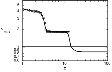
Figure 3: Plot of $v_{max}$ vs $\tau$. The maximum value of $v$ is found for two simulations with 3200 (solid line) and 20000 spatial grid points (circles) respectively. The horizontal line indicates $v=1$.

However, Fig. 3 also shows that a simulation at higher spatial resolution begins to diverge. Normally, failure of convergence signals numerical problems. Here something different is occurring. The evolution of spatial structure in $P$ depends on competition between the two nonlinear terms in the $P$ wave equation. Approximating the wave equation by $P,_{\tau\tau}+{\rm either\ of\ the\ nonlinear\ terms}=0$, a first integral can be obtained. The two potentials are $V_{1}=\pi_{Q}^{2}e^{-2P}$ and $V_{2}=e^{-2\tau}e^{2P}Q,_{\theta}^{2}$. Non-generic behavior can arise at isolated points where either $Q,_{\theta}$ or $\pi_{Q}$ vanishes. Say such a point is $\theta_{0}$. The finer the grid, the closer will be some grid point to $\theta_{0}$. Thus non-generic behavior will become more visible on a finer grid. Detailed examination shows that the differences seen in Fig. 3 are due to the slower decay of $v$ to a value below unity at isolated grid points in the higher resolution simulation.

Details of the high resolution simulation (for $0\leq\theta\leq 2\pi$) are shown in Fig. 4.

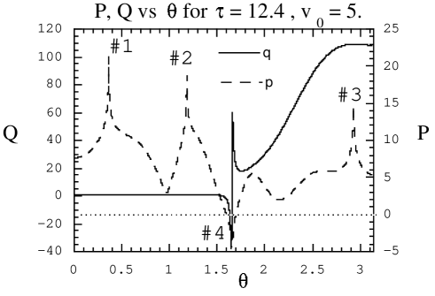
Figure 4: $P$ (dashed line) and $Q$ (solid line) vs $\theta$ at $\tau=12.4$ for the standard initial data set with $v_{0}=5$ for $0\leq\theta\leq\pi$ for a simulation containing 20000 spatial grid points in the interval $[0,2\pi]$. The numbers on the graph refer to the most interesting features. Peaks 1, 2, and 3 in P are essentially the same in that they occur where $Q,_{\theta}\approx 0$. of $Q$. Peak 4 shows an apparent discontinuity in $Q$ where $\pi_{Q}\approx 0$.

The narrow peaks in $P$ occur where $Q,_{\theta}\approx 0$. Generically, if $P\approx v\tau$ and $v>1$, the potential $V_{2}$ dominates. The relevant first integral of (4) is

$$\left(\frac{dZ}{d\tau}\right)^{2}+e^{2Z}Q,_{\theta}^{2}=const$$ (26)

where $Z=P-\tau$. A bounce off $V_{2}$ yields ${dZ}/{d\tau}\to-{dZ}/{d\tau}$ or $v-1\to 1-v$. If the new $v<0$, then $V_{1}$ dominates yielding the first integral

$$P,_{\tau}^{2}+e^{-2P}\pi_{Q}^{2}=const$$ (27)

causing $P,_{\tau}\to-P,_{\tau}$ or $v\to-v$. Eventually, bouncing between potentials gives $v<1$. However, if $Q,_{\theta}\approx 0$, but is not precisely zero, it takes a long time for the bounce off $V_{2}$ to occur. Precisely at $\theta_{0}$ (where $Q,_{\theta}=0$), $v>1$ persists. The apparent discontinuity in $Q$ is not a numerical artifact. It occurs where $P<0$ and $\pi_{Q}\approx 0$. Since $Q,_{\tau}=e^{-2P}\pi_{Q}$ and $\pi_{Q}\approx c(\theta-\theta_{0})$ (if $\pi_{Q}=0$ at $\theta_{0}$), $Q,_{\tau}$ grows exponentially in opposite directions about $\theta_{0}$. The potential $V_{1}$ drives $P$ to positive values unless $\pi_{Q}=0$. Thus this feature will narrow as the simulation proceeds.

Finally, we report a strange, and yet not understood, scaling of spatial structure in $P$ with the parameter $v_{0}$ in the initial data. In our standard initial data set, greater values of $v_{0}$ lead to the appearance of additional spatial structure in a shorter time. The rate of structure formation decreases and then stops as AVTD is approached. One may count the number of peaks in $P$ (a peak is crossed if $(P_{i+1}-P_{i})(P_{i}-P_{i-1})<0$ and $P_{i+1}<P_{i}$) during the simulation. The scaling is best for the time $\tau_{5}$ at which the 5th peak appears although it is also seen for $\tau_{3}$ and $\tau_{7}$ (the even nature of the solution causes two peaks to appear at once except at $\theta=\pi$). A plot of $1/{\tau_{5}}$ vs $v_{0}$ yields a straight line as shown in Fig. 5 which may be described as $\tau_{5}=a(v_{0}-v_{0}^{\infty})^{-1}$ where, if $v_{0}=v_{0}^{\infty}$, the 5th peak does not appear until $\tau=\infty$.

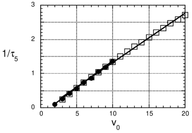
Figure 5: Scaling in the Gowdy model. Plot of $1/\tau_{5}$, the inverse of the time at which the 5th peak appears in $P$ vs $v_{0}$. Two cases are shown for initial data $P=0$, $Q=\cos\theta$: (1) $\pi_{P}=(v_{0}/\sqrt{2})\cos\theta$, $\pi_{Q}=(v_{0}/\sqrt{2})\cos\theta$ is indicated by filled circles; (2) $\pi_{P}=v_{0}\cos\theta$, $\pi_{Q}=0$ is indicated by open squares.

Even more surprisingly, almost the same line is obtained for initial data $\pi_{P}=({v_{0}}/{\sqrt{2}})\cos\theta$, $\pi_{Q}=({v_{0}}/{\sqrt{2}})\cos\theta$ rather than our standard data. Explanation of this scaling is still in progress.

5 $U(1)$ models

Moncrief has shown [17] that cosmological models on $T^{3}\times R$ with a spatial $U(1)$ symmetry can be described by five degrees of freedom $\{x,z,\Lambda,\varphi,\omega\}$ and their respective conjugate momenta $\{p_{x},p_{z},p_{\Lambda},p,r\}$. All variables are functions of spatial variables $u$, $v$ and time $\tau$ (related to distance in the symmetry direction). If we define a conformal metric $g_{ab}$ in the $u$-$v$ plane as $g_{ab}=e^{\Lambda}e_{ab}(x,z)$ where

$$e_{ab}=\frac{1}{2}\left(\begin{array}[]{cc}e^{2z}+e^{-2z}(1+x)^{2}&e^{2z}+e^{-2z}(x^{2}-1)\\ \\ e^{2z}+e^{-2z}(x^{2}-1)&e^{2z}+e^{-2z}(1-x)^{2}\end{array}\right)$$ (28)

has unit determinant and choose the lapse $N=e^{\Lambda}$, Einstein’s equations can be obtained by variation of

$$H = -\oint{\oint{du\,dv\left\{{{\textstyle{1\over 8}}p_{z}^{2}+{\textstyle{1\over 2}}e^{4z}p_{x}^{2}+{\textstyle{1\over 8}}p^{2}+{\textstyle{1\over 2}}e^{4\varphi}r^{2}-{\textstyle{1\over 2}}p_{\Lambda}^{2}-2p_{\Lambda}}\right.}}$$ (29)

$$+e^{-2\tau}\left[{\left({e^{\Lambda}e^{ab}}\right),_{ab}-\;\left({e^{\Lambda}e^{ab}}\right),_{a}\Lambda,_{b}+\;e^{\Lambda}\left({e^{-2z}}\right),_{[a}x,_{b]}}\right.$$

$$\left.{\left.{+2e^{\Lambda}e^{ab}\varphi,_{a}\varphi,_{b}+{\textstyle{1\over 2}}e^{\Lambda}e^{-4\varphi}e^{ab}\omega,_{a}\omega,_{b}}\right]}\right\}$$

$$= H_{1}+H_{2}.$$

Note particularly that

$$H_{1}=H_{1}^{G}(-2z,x)+H_{1}^{G}(-2\varphi,\omega)+H_{1}^{F}(\Lambda)$$ (30)

where $H_{1}^{G}(P,Q)$ is the kinetic part of the Gowdy Hamiltonian (20). Of course, $H_{1}^{F}$ is just a free particle Hamiltonian for the degree of freedom associated with $\Lambda$. This means that not only are the equations from $H_{1}$ exactly solvable but also that the Gowdy coding can be used with essentially no change. The potential term $H_{2}$ is very complicated. However, it still contains no momenta so its equations are trivially exactly solvable. Thus, at least in principle, the extension of the Gowdy code to the two spatial dimensions of the $U(1)$ code is completely straightforward.

There are three complications, however, which cause the $U(1)$ problem to be more difficult. The first involves the initial value problem (IVP)—the constraints must be satisfied on the initial spacelike slice. The constraints are

$${\cal H}_{0}={\cal H}-2p_{\Lambda}=0$$ (31)

(where ${\cal H}$ is the density in (29)) and

$$H_{a}=-2\tilde{\pi}^{b}_{a;b}+p_{\Lambda}\Lambda,_{a}-p_{\Lambda},_{a}+p\varphi,_{a}+r\omega,_{a}=0$$ (32)

where $\tilde{\pi}^{b}_{a}$ is in the 2-space with metric $e_{ab}$ and is linear in $p_{x}$ and $p_{z}$ with each term containing one or the other. Moncrief has proposed a particular solution to the IVP. First, identically satisfy ${\cal H}=0$ by choosing

$$p_{x}=p_{z}=\varphi,_{a}=\omega,_{a}=0\quad;\quad p_{\Lambda}=c\,e^{\Lambda}$$ (33)

for $c$ a constant. Then, solve ${\cal H}^{0}=0$ for either $r$ or $p$. Solution is possible for $c\geq c_{min}$ such that $r^{2}$ or $p^{2}\geq 0$. This allows $x$, $z$, $\Lambda$, and $p$ or $r$ to be freely specified. (Without loss of generality, it is possible to set $x=z=0$ initially to yield $e_{ab}$ flat. Such a condition may always be imposed at one time by rescaling $u$ and $v$.)

The second difficulty also involves the constraints. While the Bianchi identities guarantee the preservation of the constraints by the Einstein evolution equations, there is no such guarantee for differenced evolution equations. At this stage of the project, we monitor the maximum value of the constraints vs $\tau$ over the spatial grid but do nothing else to try to stay on the constraint hypersurface.

The third difficulty, and the one that is proving to be the greatest obstacle, is instability associated with spatial differencing in two dimensions. The differencing algorithm of section 2 for sixth order accurate expressions (based on second order ones) is used. The difficulties we encounter are apparently common to nonlinear equations in two or more dimensions. In an attempt to control the instability, we have introduced a form of spatial averaging. At the end of every time step, each value of every variable, say $\xi_{ij}$, is replaced by

$$\bar{\xi}_{i,j} = {\textstyle{1\over 2}}\xi_{i,j}+{\textstyle{1\over 4}}\left({\xi_{i+1,j}+\xi_{i-1,j}+\xi_{i,j+1}+\xi_{i,j-1}}\right)$$ (34)

$$-{\textstyle{1\over 8}}\left({\xi_{i+1,j+1}+\xi_{i-1,j-1}+\xi_{i+1,j-1}+\xi_{i-1,j+1}}\right).$$

This expression gives $\bar{\xi}_{ij}=\xi_{ij}+{\cal O}(\Delta^{4})$. In both test cases and generic models, the averaging procedure has allowed the code to run longer. However, the fact that $\bar{\xi}_{ij}\neq\xi_{ij}$ can lead to deviations of the numerical solution from the correct one. Fortunately, by comparing runs with and without averaging, these artifacts are easy to identify. We shall see some examples of how averaging can allow the code to run long enough for a conclusion about the asymptotic singularity behavior to be drawn.

Moncrief has provided a test case for the $U(1)$ code. It again starts with a polarized Gowdy solution and transforms it as either a 1D ($\theta\to u$ or $v$) or 2D ($\theta\to f(u,v)$) test problem to satisfy the $U(1)$ equations (including the constraints). As a 1D example, the agreement is excellent and the code can be run to large $\tau$. Difficulties arise in the 2D test problem in regions where the spatial derivatives are large. In application of the $U(1)$ code to generic models, AVTD models can display nonlinear wave interactions before settling down to $U\to 0$, $z,\varphi,\Lambda\to const\ \tau$, and $x,\omega\to const$. Increasing spatial resolution will yield narrower (and steeper) structures and thus may not help to cure instabilities due to steep gradients.

Nonetheless, conclusions can be drawn for generic models in our restricted class of initial data. We shall consider the models as representative of subclasses of the data. Models with $r=\omega=0$ are called polarized. This condition is compatible with the above solution and is preserved (identically) by the (analytic and numerical) evolution equations. Grubis̆ić and Moncrief have conjectured that these polarized models are AVTD [26]. Therefore, the first model is chosen to be polarized. It exhibits the conjectured AVTD behavior as shown in Figs. 6 and 7.

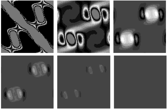
Figure 6: Frames of $U(u,v,\tau)$ for the polarized model $x=z=\Lambda=\sin u\sin v,\ p_{\Lambda}=12e^{\Lambda},\ \omega=r=0$. Time increases to the right and downward. The final frame corresponds to $U\approx 0$ everywhere.

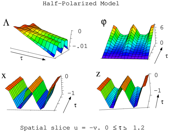
Figure 7: Surface plot of all $U(1)$ variables for the line $u=-v$ vs $\tau$ for the polarized model. Note agreement with predicted AVTD behavior that $x$ becomes constant in $\tau$ while $\Lambda$, $\varphi$, and $z$ grow linearly.

The second is generic with $p$ given and the Hamiltonian constraint solved for $r$ in the IVP. Averaging as in (34) allows the model to be followed to the point where only artifacts have $U\neq 0$. This is shown in Fig. 8.

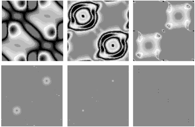
Figure 8: Frames of $U(u,v,\tau)$ for the generic model $x=z=\cos u\cos v,\ \Lambda=\sin u\sin v,\ p_{\Lambda}=14e^{\Lambda},\ p=10\cos u\cos v$ with averaging.

The last model has $r$ given with $p$ obtained by solving the Hamiltonian constraint in the IVP. Models of this type are less stable, probably due to the growth of a steep feature in $\omega$ which does not appear in the other cases. For this reason, the parameters must be kept small. Fig. 9 shows that $U\to 0$ except near artifacts where no statement can be made.

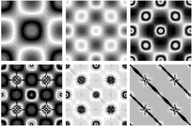
Figure 9: Frames of $U(u,v,\tau)$ for generic model $x=z=0,\ \Lambda=.1\cos u\cos v,\ p_{\Lambda}=2.1e^{\Lambda},\ r=\cos u\cos v$. The diagonal features in the final frames are numerical artifacts.

6 Conclusions

The application of the SA to Einstein’s equations for collapsing universes allows the nature of the singularity to be studied. While no real attack on Mixmaster with SA has been made, the method offers the potential for efficient, accurate evolution of this model. Application of SA to the Gowdy model has yielded strong support for its conjectured AVTD singularity and has allowed the discovery and study of interesting small scale spatial structure and scaling.

Further progress in understanding the generic singularity of $U(1)$ cosmologies requires imporvements in handling steep spatial gradients. Nevertheless there is strong support that (at least within our restricted class of initial data) polarized models are AVTD. There is also support for AVTD behavior in all generic models studied so far. Mixmaster-like bounces have not been seen. (The activity due to nonlinear wave interaction seen early in the simulations is similar to that in Gowdy models.) Several factors could account for this: (1) the BKL conjecture is false; (2) the simulations have not run long enough; (3) Mixmaster behavior is present but hidden in our variables; or (4) our class of initial data is insufficiently generic. All these possibilities will be explored in studies in progress.

Appendix

This Appendix contains a FORTRAN subroutine which uses the 6th order SA to

integrate Einstein’s equations for the Mixmaster universe:

$${{d\Omega}\over{dt}}=-p_{\Omega}\quad,\quad{{d\beta_{\pm}}\over{dt}}=p_{\pm},$$ (35)

$${{dp_{\Omega}}\over{dt}}=-\,4\,e^{4\Omega}V(\beta_{\pm})\quad,\quad{{dp_{\pm}}\over{dt}}=-\,e^{4\Omega}{{\partial V(\beta_{\pm})}\over{\partial\beta_{\pm}}}$$ (36)

where

$$V(\beta_{\pm}) = e^{-8\beta_{+}}+e^{4(\beta_{+}+\sqrt{3}\beta_{-})}+e^{4(\beta_{+}-\sqrt{3}\beta_{-})}$$ (37)

$$-2e^{4\beta_{+}}-2e^{-2(\beta_{+}+\sqrt{3}\beta_{-})}-2e^{-2(\beta_{+}+\sqrt{3}\beta_{-})}.$$

subroutine sa6(x,t,tau,param,nstate,xout)

$\ast$TAKES ONE 6TH ORDER SA STEP FROM T TO T + TAU

$\ast$

$\ast$VARIABLES: X(1) = BP, X(2) = BM, X(3) = W

$\ast$X(4) = PP, X(5) = PM, X(6) = PW

$\ast$

$\ast$XOUT CONTAINS THE OUTPUT VALUES OF THE VARIABLES

$\ast$PARAM = SQRT(3), NSTATE = 6

$\ast$

$\ast$XTEMP AND XS ARE DUMMY ARRAYS

$\ast$V IS THE POTENTIAL, DVDBP,DVDBM ARE THE GRADIENTS

$\ast$TERM_I IS AN EXPONENTIAL

$\ast$

$\ast$S, S1 ARE THE 4TH,6TH ORDER SUZUKI PARAMETERS

$\ast$DELT,DELT1 STORE T INTERVALS

parameter(mstate=20)

real$\ast$8 x(6),param(1),xout(6),xtemp(6),xs(6)

real$\ast$8 term1,term2,term3,term4,term5,term6,

&v,dvdbp,dvdbm,a,s,delt(3),s1,delt1(3)

$\ast$

$\ast$DOUBLE PRECISION IS NECESSARY

$\ast$S WAS COMPUTED WITH MATHEMATICA

s=1.35120719195965

s1=1.d0/(2.d0-2.d0$\ast$$\ast$(.2d0))

$\ast$

$\ast$STORE THE VARIABLES IN A DUMMY ARRAY

do i=1,6

xs(i) = x(i)

enddo

$\ast$

$\ast$ONE 6TH ORDER STEP IS THE PRODUCT OF 3

$\ast$4TH ORDER STEPS

$\ast$

$\ast$COMPUTE THE INTERVALS FOR THE 4TH ORDER STEPS

delt1(1) = s1$\ast$tau

delt1(2) = (1.d0-2.d0$\ast$s1)$\ast$tau

delt1(3) = s1$\ast$tau

$\ast$THE DELT1 SUM TO TAU

$\ast$

$\ast$EACH 4TH ORDER STEP IS THE PRODUCT OF 3

$\ast$2ND ORDER STEPS

$\ast$

do idel1=1,3

$\ast$

$\ast$EACH 4TH ORDER INTERVAL IS DIVIDED INTO THREE

$\ast$INTERVALS FOR 2ND ORDER

$\ast$

delt(1) = s$\ast$delt1(idel1)

delt(2) =(1.d0-2.d0$\ast$s)$\ast$delt1(idel1)

delt(3) = s$\ast$delt1(idel1)

$\ast$

do idel = 1,3

$\ast$

$\ast$PERFORM A SECOND ORDER SA STEP FOR EACH INTERVAL

$\ast$

half_tau=0.5$\ast$delt(idel)

a = param(1)

$\ast$

$\ast$EVOVLE WITH H_1 FOR HALF A TIME STEP

$\ast$

xtemp(1) = xs(1)+xs(4)$\ast$half_tau

xtemp(2) = xs(2)+xs(5)$\ast$half_tau

xtemp(3) = xs(3)-xs(6)$\ast$half_tau

$\ast$

$\ast$EVALUATE THE EXPONENTIALS IN THE MOST ACCURATE WAY

term1=exp(4$\ast$xtemp(3)-8$\ast$xtemp(1))

term2=exp(4$\ast$xtemp(3)+4$\ast$xtemp(1))

term3=exp(4$\ast$xtemp(3)+4$\ast$xtemp(1)+4$\ast$a$\ast$xtemp(2))

term4=exp(4$\ast$xtemp(3)-2$\ast$xtemp(1)-2$\ast$a$\ast$xtemp(2))

term5=exp(4$\ast$xtemp(3)+4$\ast$xtemp(1)-4$\ast$a$\ast$xtemp(2))

term6=exp(4$\ast$xtemp(3)-2$\ast$xtemp(1)+2$\ast$a$\ast$xtemp(2))

$\ast$

$\ast$COMPUTE V AND ITS GRADIENTS

v=term1+term3+term5-2.$\ast$(term2+term4+term6)

dvdbp=4.$\ast$(-2.$\ast$(term1+term2)+term3+term4

&+term5+term6)

dvdbm=4.$\ast$a$\ast$(term3+term4-term5-term6)

$\ast$

$\ast$EVOLVE WITH H_2 FOR A FULL TIME STEP

xs(4) = xs(4) - .5$\ast$dvdbp$\ast$delt(idel)

xs(5) = xs(5) - .5$\ast$dvdbm$\ast$delt(idel)

xs(6) = xs(6) - 2.$\ast$v$\ast$delt(idel)

$\ast$

$\ast$EVOLVE WITH H_1 FOR HALF A TIME STEP

$\ast$

xs(1) = xtemp(1) + xs(4)$\ast$half_tau

xs(2) = xtemp(2) + xs(5)$\ast$half_tau

xs(3) = xtemp(3) - xs(6)$\ast$half_tau

$\ast$

enddo

enddo

$\ast$

$\ast$RECORD THE DUMMY ARRAY

do i=1,6

xout(i) = xs(i)

enddo

$\ast$

return

end

OTHER CODE FEATURES:

Input w, bp, bm, pp, pm and solve H for pw.

A positive square root yields a collapsing universe.

Use an adaptive step size but require tau $\leq$ .01 t.

References

- [1] Fleck, J.A., Morris, J.R., and Feit, M.D. (1976): Time-dependent propagation of high-energy laser-beams through atmosphere. Appl. Phys. 10, 129–160
- [2] Moncrief, V. (1983): Finite-difference approach to solving operator equations of motion in quantum theory. Phys. Rev. D 28, 2485–2490
- [3] Blanco, S., Costa, A., Rosso, O.A.: Chaos in classical cosmology (II). preprint
- [4] Misner, C.W., Thorne, K.S., Wheeler, J.A. (1973): Gravitation. Freeman (San Francisco) pp. 810–813
- [5] Belinskii, V.A., Lifshitz, E.M., Khalatnikov, I.M. (1971): Oscillatory approach to the singular point in relativistic cosmology. Sov. Phys. Usp. 13, 745–765
- [6] Misner, C. W. (1969): Mixmaster universe. Phys. Rev. Lett. 22, 1071–1074
- [7] Ryan Jr., M.P., Shepley, L.C. (1975): Homogeneous Relativistic Cosmologies. Princeton University (Princeton)
- [8] Chernoff, D.F., Barrow J.D. (1983): Chaos in the Mixmaster universe. Phys. Rev. Lett. 50, 134–137
- [9] Berger, B.K. (1994): How to determine approximate Mixmaster parameters from numerical evolution of Einstein’s equations. Phys. Rev. D 49, 1120
- [10] Moser, A.R., Matzner, R.A., Ryan Jr., M.P. (1973): Numerical solutions for symmetric Bianchi IX universes. Ann. Phys. (N.Y.) 79, 558–579
- [11] Hobill, D., Burd, A., Coley, A., editors (1994): Deterministic Chaos in General Relativity. Plenum (New York)
- [12] Kasner, E. (1921): Am. J. Math. 43, 130
- [13] Gowdy, R.H. (1971): Gravitation waves in closed universes. Phys. Rev. Lett. 27 826–829
- [14] Berger, B.K. (1974): Quantum graviton creation in a model universe. Ann. Phys. (N.Y.) 83, 458
- [15] Isenberg, J., Moncrief, V. (1990): Asymptotic behavior of the gravitational field and the nature of singularities in Gowdy spacetimes. Ann. Phys. (N.Y.) 199, 84–122
- [16] Grubis̆ić, B., Moncrief, V. (1993): Asymptotic behavior of the Gowdy space-times. Phys. Rev. D 47 2371
- [17] Moncrief, V. (1986): Reduction of Einstein’s equations for vacuum space-times with spacelike isometry groups. Ann. Phys. (N.Y.) 167, 118
- [18] Suzuki, M. (1990): Fractal decomposition of exponential operators with applications to many-body theories and Monte Carlo simulations. Phys. Lett. A146, 319
- [19] Berger, B.K. (1990): Numerical study of initially expanding Mixmaster universes. Class. Quant. Grav. 7, 203–216
- [20] Berger, B.K. (1991): Comments on the computation of Liapunov exponents for the Mixmaster universe. Gen. Rel. Grav. 23, 1385–1402
- [21] Press, W.H., Flannery, B.P., Teukolsky, S.A., Vetterling, W.T. (1992): Numerical Recipes: the Art of Scientific Computing (2nd edition). Cambridge University (Cambridge)
- [22] Garcia, A.L. (1994): Numerical Methods for Physicists. Prentice-Hall (Englewood Cliffs, NJ)
- [23] Berger, B.K., Garfinkle, D., Strasser, E. unpublished
- [24] Berger, B.K., Moncrief, V. (1993): Numerical investigation of cosmological singularities. Phys. Rev. D 48, 4676
- [25] Bergr, B.K., Garfinkle, D.,Grubis̆ić, B., Moncrief, V. (1995): Phenomenology of the Gowdy Cosmology on unpublished
- [26] Grubis̆ić, B., Moncrief, V. (1994): Mixmaster spacetime, Geroch’s transformation, and constants of motion. Phys. Rev. D 49, 2792