Towards gravitational-wave asteroseismology

Abstract

We present new results for pulsating neutron stars. We have calculated the eigenfrequencies of the modes that one would expect to be the most important gravitational-wave sources: the fundamental fluid $f$-mode, the first pressure $p$-mode and the first gravitational-wave $w$-mode, for twelve realistic equations of state. From this numerical data we have inferred a set of “empirical relations” between the mode-frequencies and the parameters of the star (the radius $R$ and the mass $M$). Some of these relation prove to be surprisingly robust, and we show how they can be used to extract the details of the star from observed modes. The results indicate that, should the various pulsation modes be detected by the new generation of gravitational-wave detectors that come online in a few years, the mass and the radius of neutron stars can be deduced with errors no larger than a few percent.

1 Introduction

1.1 Motivation

The day of the first undeniable detection of gravitational waves should not be far away. In less than five years at least five large interferometric gravitational-wave detectors (LIGO, VIRGO, GEO600 and TAMA) will be operating. At the same time a new generation of spherical resonant detectors (GRAIL, SFERA etc) could be sensitive enough to detect signals from supernova collapse and binary coalescences in the Virgo cluster of galaxies. In other words: Recent advancements in technology are heralding the era of gravitational-wave astronomy. However, for this field to reach its full potential theoreticians must in advance point out the most promising sources, the optimal methods of detection and the appropriate bandwidth to which the detectors should be tuned. Hence, the theoretical effort is presently focused on various sources of potentially detectable gravitational waves, in order to both characterize the waves and device detailed detection strategies. Once gravitational waves are detected the first task will be to identify the source. This should be possible from the general character of the waveform and may not require very accurate theoretical models, but accurate models will be of crucial importance for a deduction of the parameters of the source. That is, for gravitational-wave “astronomy”.

With this paper we contribute to this rapidly growing field in two ways. We present results for the gravitational waves from a pulsating relativistic star, eg. the violent oscillations of a compact object formed after a core collapse. These results provide a means for taking the fingerprints of the source, and suggest optimal bandwidths to which a detector should be tuned to enable detection of such signals. Specifically, we discuss how the information carried by gravitational waves from a pulsating star can be used to infer, with good precision, both the mass and the radius of the star: Data that would strongly constrain the supranuclear equation of state (EOS).

The idea behind the present work is a familiar one in astronomy: For many years, studies of the light variation of variable stars have been used to deduce their internal structure [1989]. The Newtonian theory of stellar pulsation was to a large extent developed in order to explain the pulsations of Cepheids and RR Lyrae. This approach, known as Asteroseismology (Helioseismology in the specific case of the Sun), has been quite successful in recent years. The relativistic theory of stellar pulsation has now been developed for thirty years, but it has not yet been applied in a similar way. So far, the relativistic theory has no immediate connections to observations (that are not already provided by the Newtonian theory). We believe that this situation will change once the gravitational-wave window to the universe is opened, and with this article we discuss how the information carried by the gravitational-wave signal can be inverted to estimate the parameters of pulsating stars. That is, we take the first (small) step towards gravitational-wave asteroseismology.

1.2 Detectability of the waves

At the present time it is not clear that the gravitational waves from pulsating neutron stars will be seen by the detectors that are presently under construction. Our relative ignorance in this matter is due to the lack of accurate, fully relativistic, models of, for example, the gravitational collapse that follows a supernova. At present we simply do not know how much energy will be radiated through the oscillation modes of a nascent neutron star. But one can argue that the released energy could be considerable. One generally expects the newly formed neutron star to pulsate wildly during the first few seconds following the collapse. This pulsation will be damped mainly through gravitational waves. This means that the signal, that carries the signature of the collapsed object, may be invisible in the electromagnetic spectrum, but the amplitude of the emerging gravitational waves could be considerable. The energy stored in the pulsation can potentially be of the same order as the kinetic energy of the collapse. In fact, it is not unreasonable to expect that a significant part of the mass energy of the newly formed object is radiated in this way.

The spectrum of a pulsating relativistic star is tremendously rich, since essentially every feature of the star can be directly associated with (at least) one distinct family of pulsation modes [1988, 1996]. But it seems likely that only a few of these modes will carry away the bulk of the radiated energy [1997]. From the gravitational-wave point of view, the most important modes are the fundamental ($f$) mode of fluid oscillation, the first and maybe the second pressure ($p$) modes and the first gravitational-wave ($w$) mode [1992, 1995, 1996]. Other pulsation modes, eg. the $g$ (gravity), higher order $p$-modes, $s$ (shear), $t$ (toroidal), $i$ (interface) modes, can be accounted for with Newtonian dynamics since they do not emit significant amounts of gravitational radiation [1988]. For a historical description of, and further details on, the theory of relativistic stellar pulsation we refer the reader to a recent review article by one of us [1997]. A detailed discussion of the relativistic perturbation equations was recently provided by Allen et al. [1997].

The pulsation modes of a neutron star are likely to be excited in many dynamical processes, but will the resultant gravitational waves be strong enough to be detectable on Earth? As already mentioned, the answer to that question is unclear and demands more accurate modeling, but it is straightforward to derive useful order of magnitude estimates. As we have have recently shown elsewhere [1996], we get

$$h_{\rm eff}\sim 2.2\times 10^{-21}\left({E\over 10^{-6}M_{\odot}c^{2}}\right)^{1/2}\left({2{\rm kHz}\over f}\right)^{1/2}\left({50{\rm kpc}\over r}\right)\ ,$$ (1)

for the $f$-mode, and

$$h_{\rm eff}\sim 9.7\times 10^{-22}\left({E\over 10^{-6}M_{\odot}c^{2}}\right)^{1/2}\left({10{\rm kHz}\over f}\right)^{1/2}\left({50{\rm kpc}\over r}\right)\ ,$$ (2)

for the fundamental $w$-mode. Here we have used typical parameters for the pulsation modes, $E$ is the available pulsation energy, and the distance scale used is that to SN1987A. In this volume of space one would not expect to see more than one event per ten years or so. However, the assumption that the energy released through gravitational waves in a supernova is of the order of $10^{-6}M_{\odot}c^{2}$ is probably conservative. If a substantial fraction of the binding energy of a neutron star were released through the pulsation modes they could potentially be observable all the way out to the Virgo cluster. Then we could hope to see several events per year.

Suppose we want to know how much energy must go into each mode to achieve an effective gravitational-wave amplitude $h_{\rm eff}\sim 10^{-21}$ (the order of magnitude a signal must have to be “detectable”) when the source is at a distance of 15 Mpc. We can invert the above relations, and find that at least 1% of a solar mass must be radiated through these modes if they are to be detectable at the Virgo distance. The specific numbers are $E\approx 0.019M_{\odot}c^{2}$ for the $f$-mode and $E\approx 0.096M_{\odot}c^{2}$ for the $w$-mode. To assume that this amount of energy actually goes into these modes seems somewhat optimistic, but the possibility should not be ruled out. Anyway, the rough estimates indicate that the pulsations of a nascent neutron star in the local group of galaxies could well be detectable. This may not be a very frequent event, but as we shall see the pay-off of its detection could be great.

1.3 Addressing the inverse problem

Considering the possibility of a future detection it is relevant to pose the “inverse problem” for gravitational waves from pulsating stars. Once we have observed the waves, can we deduce the details of the star from which they originated? To answer this question we have calculated the frequencies and damping times of the modes that we expect to lead to the strongest gravitational waves for a selection of EOS. The numerical method used for the calculation is essentially that described by Andersson, Kokkotas and Schutz [1995]. The study includes several stellar models for each EOS. The obtained data, which is tabulated in Appendix A, extends previous results of Lindblom and Detweiler [1983] in two ways: i) a few modern EOS are included, and ii) we have added results both for $p$- and $w$-modes. We have used this numerical data to create useful “empirical” relations between the “observables” (frequencies and damping times) and the parameters of the star (mass, radius and possibly the EOS). As we will show in the following, these relations can be used to infer the stellar parameters from detected mode data.

In this study we have not taken into account the effects of rotation. There are two reasons for this: Firstly, rotation should have a marginal effect, except for in the most rapidly spinning cases, since rotational effects scale as the angular velocity squared. Secondly, and more importantly, there is at present no available method that can be used to study pulsation modes of a rapidly rotating relativistic star. Such methods must be developed, and once the relevant results become available the present study can be complemented to incorporate them.

Before we proceed to discuss the deduced empirical relations, a few comments on our choice of stellar models are in order. In Appendix A we tabulate data for various oscillation modes ($f$, $p$ and $w$) for twelve different EOS listed in Table 1. The chosen pulsation modes are those that i) should produce the strongest gravitational waves, and ii) lie inside the bandwidth of the detectors which are either planned or under construction. Most of the EOS were taken from the old Arnett and Bowers catalogue [1974]. Although some of these EOS might be outdated none of them are ruled out by present observations. Furthermore, the range of stiffness of the EOS listed by Arnett and Bowers is still relevant today. This is important for the present study: In order for our analysis to be robust it is necessary that our sample of EOS spans the anticipated range of stiffness. However, we have also included three more modern EOS: one of the models of Wiringa et al [1988] and two models from Glendenning [1985]. For the EOS that were also considered by Lindblom and Detweiler [1983] we have chosen identical stellar models to facilitate a comparison of the results. Finally, we have only included stellar models whose masses and radii are within the limits accepted by current observations [1994, 1995].

Table 1: The twelve Equations of State that were included in the study.

Model	Reference
A	Pandharipande [1971] (neutron)
B	Pandharipande [1971] (hyperonic; model C)
C	Bethe and Johnson [1974] (model I)
D	Bethe and Johnson [1974] (model V)
E	Moszkowski [1974]
F	Arponen [1972]
G	Canuto and Chitre [1974]
I	Cohen et al. [1970]
L	Pandharipande et al. [1976]
WFF	Wiringa et al.[1988]
G240	Glendenning [1985] K240
G300	Glendenning [1985] K300

2 What can we learn from observations?

Our present understanding of neutron stars comes mainly from X-ray and radio-timing observations. These observations provide some insight into the structure of these objects and the properties of supranuclear matter. The most commonly and accurately observed parameter is the rotation period, and we know that radio pulsars can spin very fast (the shortest observed period being the 1.56 ms of PSR 1937+21). Another basic observable, that can be obtained (in a few cases) with some accuracy from todays observations, is the mass of the neutron star. As Finn [1994] has shown, the observations of radio pulsars indicate that $1.01<{M/M_{\odot}}<1.64$. Similarly, van der Kerkwijk et al [1995] find that data for X-ray pulsars indicate $1.04<{M/M_{\odot}}<1.88$. The data used in these two studies is actually consistent with (if one includes error bars) $M<1.44M_{\odot}$. We now recall that the various EOS that have been proposed by theoretical physicists can be divided into two major categories: i) the “soft” EOS which typically lead to neutron star models with maximum masses around $1.4M_{\odot}$ and radii usually smaller than 10 km, and ii) the “stiff” EOS with the maximum values $M\sim 1.8M_{\odot}$ and $R\sim 15$ km [1977]. From this one can deduce that, even though the constraint put on the neutron star mass by present observations seems strong, it does not rule out many of the proposed EOS. In order to arrive at a more useful result we are likely to need detailed observations also of the stellar radius. Unfortunately, available data provide little information about the radius. The recent observations of quasiperiodic oscillations in low mass X-ray binaries indicate that $R<6M$, but again this is not a severe constraint. Although a number of attempts have been made, using either X-ray observations [1993] or the limiting spin period of neutron stars [1986], to put constraints on the mass-radius relation, we do not yet have a method which can provide the desired answer.

2.1 A detection scenario

In view of this situation, any method that can be used to infer neutron star parameters is a welcome addition. Of specific interest may be the new possibilities offered once gravitational-wave observations become reality. An obvious question is to what extent one can solve the inverse problem in gravitational-wave astronomy. In this paper we address this issue for the case of waves from pulsating neutron stars. In Appendix A we provide extended tables with frequencies and damping times for the most relevant pulsation modes (as far as gravitational waves are concerned) of various stellar models created from a range of realistic EOS. We will suppose that these modes can be detected by some future generation of gravitational-wave detectors, and investigate to what precision we can hope to calculate the parameters of the source from observed data.

Let us suppose that a nearby supernova explodes, say in the Local Group of galaxies, and is followed by a core collapse that leads to the formation of a compact object. As the dust from the collapse settles the compact object pulsates wildly in its various oscillation modes, generating a gravitational-wave signal which is composed of an overlapping of different frequencies.. We will assume that the results of Allen et al [1997] can be brought to bear on this situation, i.e. that most of the energy is radiated through the $f$-mode, a few $p$-modes and the first $w$-mode. Our detector picks up this signal, and a subsequent Fourier analysis of the data stream yields the frequencies and the energy content in each mode.

The first question to be answered by the gravitational-wave astronomer concerns what kind of compact object could produce the detected signal. Is it a black hole or a neutron star? The pulsation of these objects lead to qualitatively similar gravitational waves, eg. exponentially damped oscillations, but the question should nevertheless be relatively easy to answer. If more than one of the stellar pulsation modes is observed the answer is clear, but even if we only observe only one single mode the two cases should be easy to distinguish. The fundamental (quadrupole) quasinormal mode frequency of a Schwarzschild black hole follows from

$$f\approx 12{\rm kHz}\left({M_{\odot}\over M}\right),$$ (3)

while the associated e-folding time is

$$\tau\approx 0.05{\rm ms}\left({M\over M_{\odot}}\right)\ .$$ (4)

That is, the oscillations of a 10 $M_{\odot}$ black hole lie in the frequency range of the $f$-mode for a typical neutron star (see Appendix A). But the two signals will differ greatly in the damping time, the e-folding time of the black hole being nearly three orders of magnitude shorter than that of the neutron star $f$-mode.

Having excluded the possibility that our signal came from a black hole, we want to know the mass and the radius of the newly born neutron star. We also want to decide which of the proposed EOS that best represents this star. To address these questions we can use a set of empirical relations deduced from the data of Appendix A: Relations that can be used to estimate the mass, the radius and the EOS of the neutron star with good precision.

2.2 Empirical relations

Let us first consider the frequency of the $f$-mode. It is well known that the characteristic time-scale of any dynamical process is related to the mean density of the mass involved (see Misner, Thorne and Wheeler [1973] ch. 36.2). This notion should be relevant for the fluid oscillation modes of a star, and we consequently expect that $\omega_{f}\sim\bar{\rho}^{1/2}$. That is, we should normalize the $f$-mode frequency with the average density of the star. The result of doing this is shown in Figure 1. From this Figure it is apparent that the relation between the $f$-mode frequencies and the mean density is almost linear, and a linear fitting leads to the following simple relation:

$$\omega_{f}(kHz)\approx 0.78+1.635\left({{\bar{M}}\over{{\bar{R}}^{3}}}\right)^{1/2}\ ,$$ (5)

where we have introduced the dimensionless variables

$${\bar{M}}={M\over{1.4M_{\odot}}}\quad\mbox{and}\quad{\bar{R}}={R\over 10{\rm km}}\ .$$ (6)

¿From equation (5) follows that the typical $f$-mode frequency is around 2.4 kHz.

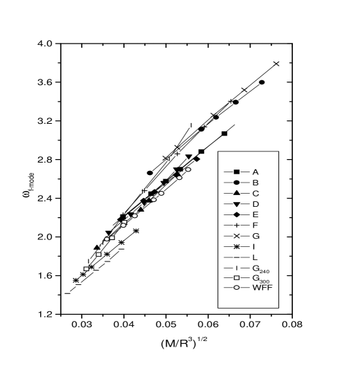
Figure 1: The numerically obtained $f$-mode frequencies plotted as functions of the mean stellar density ($M$ and $R$ are in km and $\omega_{f-mode}$ in kHz).

To deduce a corresponding relation for the damping rate of the $f$-mode, we can use the rough estimate given by the quadrupole formula. That is, the damping time should follow from

$$\tau_{f}\sim{\mbox{oscillation energy}\over{\mbox{power emitted in GWs}}}\sim R\left({R\over M}\right)^{3}\ .$$ (7)

Using this normalization we plot the functional $(\tau_{f}M^{3}/R^{4})^{-1}$ as a function of the stellar compactness, cf. Figure 2. The data shown in this Figure leads to a relation between the damping time of the $f$-mode and the stellar parameters $M$ and $R$:

$${1\over\tau_{f}({\rm s})}\approx{{\bar{M}}^{3}\over{\bar{R}}^{4}}\left[22.85-14.65\left({{\bar{M}}\over{\bar{R}}}\right)\right]\ .$$ (8)

The small deviation of the numerical data from the above formula is apparent in Figure 2, and one can easily see that a typical value for the damping time of the $f$-mode is a tenth of a second.

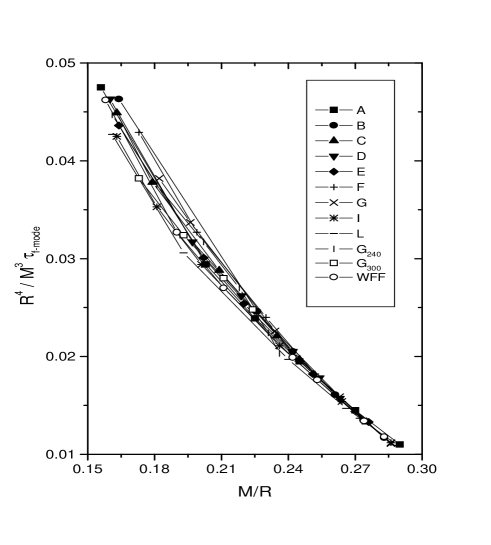
Figure 2: The normalized damping time of the $f$-modes as function of the stellar compactness ($M$ and $R$ are in km and $\tau_{f-mode}$ in secs).

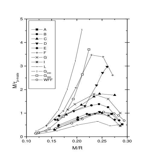
Figure 3: The damping time of the $p$-modes as function of the stellar compactness ($M$ and $R$ are in km and $\tau_{p-mode}$ in secs).

For the damping rate of the $p$-modes the situation is not so favorable. This is because the damping of the $p$-modes is more sensitive to changes in the modal distribution inside the star. Thus, different EOS lead to rather different $p$-mode damping rates, cf. Figure 3. Previous evidence for polytropes [1997] actually indicate that this would be the case. Clearly, an empirical relation based on the data in Figure 3 would not be very robust.

The situation is slightly better if we consider the oscillation frequency of the $p$-mode. From the data graphed in Figure 4 we can deduce a relation between the $p$-mode frequency and the parameters of the star:

$$\omega_{p}({\rm kHz})\approx{1\over{{\bar{M}}}}\left(1.75+5.59{{\bar{M}}\over{{\bar{R}}}}\right)\ ,$$ (9)

and we see that a typical $p$-mode frequency is around 7 kHz. Although the data for several EOS deviate significantly from (9) it is still a useful result. Stellar masses and radii deduced from it will not be as accurate as ones based on $f$-mode data, but on the other hand, if $M$ and $R$ are obtained in some other way (say, from a combination of observed $f$- and $w$-modes) the $p$-mode can be used to deduce the relevant EOS.

Figure 4: The $p$-mode frequencies plotted a function of the compactness of the star ($M$ and $R$ are in km and $\omega_{p-mode}$ in kHz).

That empirical relations based on $p$-mode data would be less robust and useful than those for the $f$-mode was expected, since the $p$-modes are sensitive to changes in the matter distribution inside the star. In contrast, the gravitational-wave $w$-modes should lead to very robust results. It is well known [1992, 1996] that the $w$-modes do not excite a significant fluid motion. Thus, they are more or less independent of the characteristics of the fluid: The frequencies do not depend on the sound speed and the damping times cannot be modeled by the quadrupole formula. But we can nevertheless deduce the appropriate normalization for the $w$-mode data listed in Appendix A. Analytic results for model problems for the $w$-modes [1986, 1996], show that the frequency of the $w$-mode is inversely proportional to the size of the star. This is clear from the data in Figure 5. Meanwhile, the damping time is related to the compactness of the star, i.e. the more relativistic the star is the longer the $w$-mode oscillation lasts. This is shown in Figure 6. These properties have already been discussed in some detail by Andersson, Kojima and Kokkotas [1996] for uniform density stars.

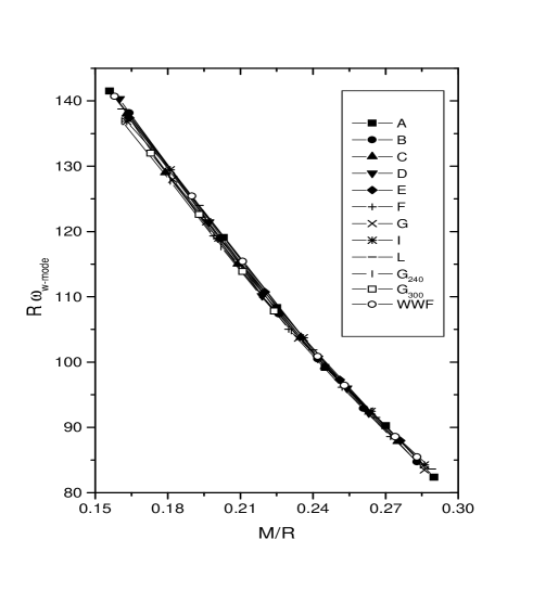
Figure 5: The functional $R\omega_{w}$ as function of the compactness of the star ($M$ and $R$ are in km and $\omega_{w-mode}$ in kHz).

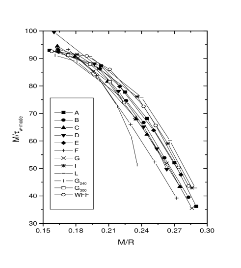
Figure 6: The functional $M/\tau_{w}$ as function of the compactness of the star ($M$ and $R$ are in km and $\tau_{w-mode}$ in msecs).

For the present numerical data (shown in Figures 5 and 6) we find the following relations for the frequency and damping of the first $w$-mode:

$$\omega_{w}({\rm kHz})\approx{1\over{\bar{R}}}\left[20.92-9.14\left({\bar{M}}\over{\bar{R}}\right)\right]\ ,$$ (10)

and

$${1\over\tau_{w}({\rm ms})}\approx{1\over{\bar{M}}}\left[5.74+103\left({{\bar{M}}\over{\bar{R}}}\right)-67.45\left({{\bar{M}}\over{\bar{R}}}\right)^{2}\right]\ .$$ (11)

We see that a typical value for the $w$-mode frequency is 12 kHz, but since the frequency depends strongly on the radius of the star it varies greatly for different EOS. For example, for a very stiff EOS (L) the $w$-mode frequency is around 6 kHz while for the softest EOS in our set (G) the typical frequency is around 14 kHz. The $w$-mode damping time is comparable to that of an oscillating black hole with the same mass, i.e. it is typically less than a tenth of a millisecond.

2.3 A simple experiment

In principle, the relations we have deduced between the various pulsation modes and the stellar parameters can be used to infer $M$ and $R$ (or some combination thereof) from detected mode-data. The five relations (5) — (11) form an over-determined system of five equations for the two unknown quantities $R$ and $M$. One would expect this system to provide an accurate characterization of the star in the ideal case when the gravitational-wave signal carries energy in all modes ($f$, $p$ and $w$).

This idea is promising and simple enough, but we need to examine how well it can work in practice. To do this we have constructed a set of independent polytropic stellar models ($p=K\rho^{1+1/N}$) with varying polytropic indices ($N=0.8;1;1.2$). We have determined the $f$-mode, the first $p$-mode and the slowest damped $w$-mode for each of these models. We let this data represent “observed” gravitational-wave signals, and use various combinations of the relations (5) – (11) to extract the values of the masses and radii of the stellar models.

In Figure 7 we show the result of a combination of the relations for $f$- and $w-$modes [(5), (8), (10) and (11)] for one of the polytropic models. In the Figure, a filled circle represents the true parameters of the star, and it is clear that estimates based on the above relations can be very accurate. More detailed results are listed in Table 2. The typical errors of a parameter estimation based on the oscillation frequencies of the $f$- and the $w$-mode [the combination of (5) and (10)] are (5% ,2%) where the first number is the error in the radius and the second is the error in the mass. Combining the frequency and damping of the $f$-mode [(5) and (8)] we find (6.5% ,17.6%). The $f$-mode frequency and the $w$-mode damping rate [(5) and (11)] lead to (5.6% ,1.4%), while the $w$-mode frequency and the $f$-mode damping [(10) and (8)] yield (3.2% ,1.9%). A combination of the $w$-mode frequency and damping rate [(10) - (11)] leads to (3.9% ,1.6%). Finally, by combining the damping rates of the $f$- and the $w$-mode [(11) and (8)] we get (2.1% ,6.3%). These results are rather impressive. The robustness of our empirical relations for $f$- and $w$-modes, and the precision with which they can be used to deduce stellar masses and radii, is surprising. The errors are notably larger when we replace either the $f$- or the $w$-mode with the $p$-mode. For example, for the combination (5) and (9), the oscillation frequencies of the $f$- and $p$-modes, the method estimates the stellar parameters to within (23%,123%). That is, from this combination we can at best get upper and lower bounds of the parameters of the observed object.

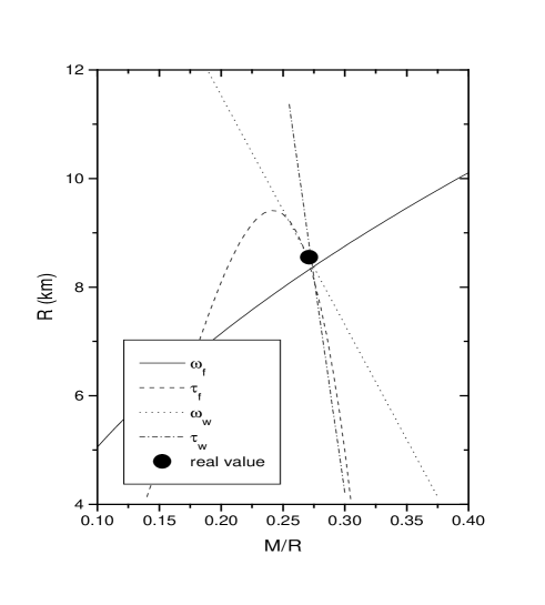
Figure 7: An illustration of how accurately the radius and the mass of a star can be inferred from detected mode data and our empirical relations.

Table 2: Results from a simple “experiment”: We have used the empirical relations for mode-frequencies of realistic EOS to deduce the stellar parameters of a set of independent polytropic models. In the first three columns we list the parameters of the polytropes: the polytropic index, the radius and the mass. The following columns give the percentage error in the estimated parameters (radius,mass) when the polytropic mode-frequencies are used in our relations for $f$- and $w$-modes [(5),(8), (10) and (11)]. We have not used the $p$-mode data here, since the corresponding empirical relations are less robust than for the other modes.

$N$	$R(km)$	$M(M_{\odot})$	(5) and (10)	(5) and (8)	(5) and (11)	(10) and (8)	(10) and (11)	(11) and (8)
0.8	10.03	1.08	(-3.5 , 0.1)	( -5.3 ,- 5.4)	(-3.9 ,-1.3)	(-2.6 ,-1.0)	(-2.2 ,-1.3)	( -2.8 , -1.3)
0.8	9.49	1.35	(-0.02,-1.8)	( 4.7 , 11.8)	( 0.8 , 0.6)	(-4.6 ,-0.6)	(-2.9 ,-1.1)	( -1.5 , -0.5)
0.8	8.99	1.50	( 1.3 ,-1.1)	( 0.1 , -5.1)	( 2.1 , 1.1)	(-6.8 ,-1.6)	(-1.6 ,-1.4)	( 0.6 , 0.02)
1.0	9.65	1.13	( 3.4 ,-4.0)	( 9.7 , 15.2)	( 4.4 ,-0.6)	(-0.5 ,-1.5)	(-0.3 ,-1.6)	( -0.5 , -1.7)
1.0	8.86	1.27	( 6.6 ,-3.0)	( -3.5 ,-40.0)	( 7.9 , 1.5)	(-1.7 ,-2.5)	( 1.9 ,-2.0)	( -0.8 ,-28.9)
1.0	7.42	1.35	( 9.7 , 2.7)	( 10.9 , 6.6)	(10.2 , 4.2)	(-4.4 ,-1.4)	( 7.7 , 1.9)	( 4.3 , -8.7)
1.2	12.77	1.24	(-1.6 , 1.6)	(-12.0 ,-32.0)	(-2.5 ,-0.9)	( 3.0 ,-4.2)	( 0.7 ,-1.5)	( 4.4 , -1.8)
1.2	10.48	1.44	( 7.4 ,-3.5)	( -2.2 ,-38.7)	( 7.8 ,-1.9)	( 3.8 ,-3.0)	( 5.6 ,-3.2)	( -3.2 , -4.7)
1.2	8.97	1.46	(11.4 , 0.3)	( 10.3 , -3.4)	(11.2 ,-0.2)	( 1.8 ,-1.5)	(12.0 , 0.5)	( 1.3 , -8.9)

That the $p$-mode relation is less useful for an inversion to yield the stellar mass and radius is, however, not completely bad news. Once we have estimated the mass and the radius we want to identify which of the proposed EOS that best fits the observed data. When combined with data deduced from the other modes the $p$-modes can provide the answer to this question, eg. via the results in Figure 3. If we observe a $p$-mode we should at least be able to exclude the unsuitable EOS.

The most suitable EOS can, of course, also be deduced from the mass and radius of the star. As we show in Figure 8 the mass-radius relation is characteristic for each EOS in our sample. From this data it should not be difficult to infer which EOS that can lead to a mass and radius obtained via the empirical relations. Alternatively, one can use the approach suggested by Lindblom [1992]. He has shown how one can reconstruct the density-pressure relation in the interior of a neutron star from a sample of observed masses and radii.

Figure 8: The mass-radius relation for the twelve EOS in our sample. This data can be used to identify which of the EOS that agrees best with the estimated parameters of a star. From the graph one can easily identify the relative stiffness of the EOS. In order of increasing stiffness they can be ordered $G<B<F<A<E<D<WFF<C<G_{240}<G_{300}<I<L$.

3 Concluding remarks

This paper concerns the feasibility of gravitational-wave asteroseismology. That is, whether it is realistic to expect to be able to infer stellar parameters [mass, radius and EOS] from observations of gravitational-wave signals from pulsating neutron stars. To address this issue we have calculated the details of the modes that we expect to provide the strongest gravitational waves: the $f$-mode, the first $p$-mode and the first $w$-mode, for a sample of twelve realistic EOS. Our chosen EOS span a range of stiffness that should include all proposed models. From the obtained data we have deduced a set of empirical relations that can be used to infer the mass and the radius (or rather, combinations thereof) from observed mode-frequencies. In the ideal case, when both the $f$- and the $w$-mode are detected, our empirical relations predict $M$ and $R$ with surprising precision.

These results are undoubtedly interesting, but so far we have discussed an ideal scenario. In order for gravitational-wave asteroseismology to become reality, the detectors that are presently under construction or at the planning stage must be able to detect these mode-signals. We have argued that this may be possible in a hand-waving way, but we have as yet no detailed results. The answer depends to a large extent on how much energy is radiated through the pulsation modes of, for example, a nascent neutron star immediately following the collapse. At the present time there are no reliable predictions of this, and fully relativistic collapse simulations are desperately needed. This is a challenge for numerical relativity, and hopefully the answer will be known in the near future. Another, related issue, that we have not addressed concerns the expected detection errors. When the signal is noisy, as is likely to be the case, there will be statistical errors associated with the observed mode-data. These errors will obviously affect the precision with which the stellar parameters can be deduced from our empirical relations.

Finally, the detectors which will be in operation in the next decade will mainly be sensitive to frequencies below 5-6 kHz. The $f$-modes are well inside this bandwidth, as is the first $p$-mode for most of the EOS we have considered. But only for the stiffest EOS does the first $w$-mode have a frequency around 6 kHz. This is bad news for the proposed parameter detection/inversion. But as we have seen, a detection of the $w$-mode could lead to a very accurate deduction of the stellar mass and radius. The astrophysical pay-off would thus be considerable, and the situation illustrates the need to complement the currently planned detectors with ones dedicated to a search for high-frequency gravitational waves.

Appendix A Results for various Equations of State

This appendix provides the numerical data for mode-frequencies of 12 realistic EOS. This data was used to infer the empirical relations discussed in the main body of the paper. We provide the data in the form of one table for each EOS. In each table we list the central density, the radius and the mass of the stellar model and the frequencies and the damping times of the $f$-mode, the first $p$-mode and the first $w$-mode.

Table 3: Data for the EOS A, (Pandharipande 1971)

$\rho_{c}\times 10^{15}$	$R$	$M$	$\omega_{f}$	$\tau_{f}$	$\omega_{p}$	$\tau_{p}$	$\omega_{w_{0}}$	$\tau_{w}$
$gr/cm^{3}$	$km$	$M_{\odot}$	kHz	s	kHz	s	kHz	ms
3.980	8.426	1.653	3.090	0.109	7.838	4.640	9.824	0.064
3.000	8.884	1.620	2.888	0.106	7.822	2.475	10.165	0.045
2.344	9.268	1.535	2.704	0.109	7.819	2.163	10.766	0.032
1.995	9.493	1.447	2.579	0.117	7.818	2.293	11.444	0.027
1.698	9.688	1.328	2.447	0.132	7.807	2.726	12.344	0.022
1.259	9.924	1.050	2.203	0.183	7.543	5.218	14.328	0.017

Table 4: Data for the EOS B, (Pandharipande 1971)

$\rho_{c}\times 10^{15}$	$R$	$M$	$\omega_{f}$	$\tau_{f}$	$\omega_{p}$	$\tau_{p}$	$\omega_{w}$	$\tau_{w}$
$gr/cm^{3}$	$km$	$M_{\odot}$	kHz	s	kHz	s	kHz	ms
5.012	7.317	1.405	3.598	0.091	8.957	2.994	11.577	0.053
7.684	7.682	1.360	3.393	0.089	8.739	1.615	12.094	0.037
3.388	7.951	1.303	3.236	0.091	8.515	1.406	12.638	0.029
3.000	8.143	1.248	3.113	0.095	8.314	1.403	13.183	0.025
1.995	8.761	0.971	2.661	0.144	7.467	1.635	15.770	0.015

Table 5: Data for the EOS C, (Bethe & Johnson 1974) (model I)

$\rho_{c}\times 10^{15}$	$R$	$M$	$\omega_{f}$	$\tau_{f}$	$\omega_{p}$	$\tau_{p}$	$\omega_{w}$	$\tau_{w}$
$gr/cm^{3}$	$km$	$M_{\odot}$	kHz	s	kHz	s	kHz	ms
3.0	9.952	1.852	2.656	0.121	6.432	1.548	8.843	0.062
1.995	10.778	1.790	2.383	0.124	6.209	1.452	9.214	0.040
1.778	11.009	1.746	2.304	0.129	6.126	1.514	9.444	0.035
1.413	11.441	1.619	2.144	0.146	5.925	1.766	10.124	0.028
1.122	11.832	1.435	1.975	0.181	5.664	2.264	11.003	0.023
1.0	12.017	1.322	1.885	0.208	5.505	2.741	11.496	0.021

Table 6: Data for the EOS D, (Bethe & Johnson 1974) (model V)

$\rho_{c}\times 10^{15}$	$R$	$M$	$\omega_{f}$	$\tau_{f}$	$\omega_{p}$	$\tau_{p}$	$\omega_{w}$	$\tau_{w}$
$gr/cm^{3}$	$km$	$M_{\odot}$	kHz	s	kHz	s	kHz	ms
3.548	9.262	1.652	2.833	0.108	6.646	0.822	9.954	0.049
3.0	9.597	1.649	2.699	0.110	6.662	0.900	10.001	0.043
2.512	9.945	1.632	2.560	0.114	6.456	1.106	10.114	0.037
1.778	10.448	1.549	2.356	0.127	5.911	1.763	10.543	0.029
1.413	10.678	1.425	2.235	0.147	5.881	1.945	11.371	0.024
1.122	10.968	1.187	2.045	0.194	5.351	2.455	12.792	0.019

Table 7: Data for the EOS E, (Moszkowski 1974)

$\rho_{c}\times 10^{15}$	$R$	$M$	$\omega_{f}$	$\tau_{f}$	$\omega_{p}$	$\tau_{p}$	$\omega_{w}$	$\tau_{w}$
$gr/cm^{3}$	$km$	$M_{\odot}$	kHz	s	kHz	s	kHz	ms
2.818	9.171	1.713	2.805	0.109	7.553	3.503	9.593	0.053
2.239	9.562	1.626	2.642	0.111	7.474	2.372	10.175	0.038
1.778	9.915	1.476	2.467	0.123	7.327	2.256	11.170	0.027
1.585	10.066	1.378	2.376	0.135	7.212	2.476	11.812	0.024
1.259	10.316	1.145	2.180	0.179	6.865	3.404	13.321	0.018

Table 8: Data for the EOS F, (Arponen 1972)

$\rho_{c}\times 10^{15}$	$R$	$M$	$\omega_{f}$	$\tau_{f}$	$\omega_{p}$	$\tau_{p}$	$\omega_{w}$	$\tau_{w}$
$gr/cm^{3}$	$km$	$M_{\odot}$	kHz	s	kHz	s	kHz	ms
5.012	7.966	1.464	3.403	0.097	7.349	0.826	11.123	0.0551
3.981	8.495	1.450	3.138	0.098	7.087	0.631	11.318	0.0409
3.162	9.087	1.413	2.859	0.104	6.855	0.601	11.560	0.0316
2.239	9.934	1.335	2.478	0.130	6.585	0.948	12.011	0.0235
1.585	10.462	1.225	2.231	0.157	6.361	1.653	12.655	0.0194
1.122	10.892	1.031	1.980	0.475	6.039	3.194	13.705	0.0167

Table 9: Data for the EOS G, (Canuto & Chitre 1974)

$\rho_{c}\times 10^{15}$	$R$	$M$	$\omega_{f}$	$\tau_{f}$	$\omega_{p}$	$\tau_{p}$	$\omega_{w}$	$\tau_{w}$
$gr/cm^{3}$	$km$	$M_{\odot}$	kHz	s	kHz	s	kHz	ms
6.042	7.010	1.356	3.801	0.091	9.029	1.994	11.931	0.056
4.503	7.472	1.327	3.526	0.087	8.722	1.223	12.402	0.037
3.498	7.898	1.253	3.264	0.091	8.387	1.024	13.146	0.026
2.631	8.397	1.114	2.927	0.111	7.897	1.194	14.556	0.019
2.376	8.556	1.057	2.813	0.123	7.705	1.360	15.069	0.017

Table 10: Data for the EOS I, (Cohen et al. 1970)

$\rho_{c}\times 10^{15}$	$R$	$M$	$\omega_{f}$	$\tau_{f}$	$\omega_{p}$	$\tau_{p}$	$\omega_{w}$	$\tau_{w}$
$gr/cm^{3}$	$km$	$M_{\odot}$	kHz	s	kHz	s	kHz	ms
1.585	12.468	2.418	2.063	0.158	5.444	7.729	6.758	0.083
1.259	13.023	2.324	1.943	0.154	5.415	3.796	7.100	0.058
1.0000	13.498	2.154	1.822	0.163	5.358	3.270	7.685	0.042
0.7943	13.885	1.894	1.689	0.193	5.255	3.736	8.571	0.032
0.6310	14.128	1.562	1.551	0.255	5.087	5.294	9.686	0.025

Table 11: Data for the EOS L, (Pandharipande et al. 1976)

$\rho_{c}\times 10^{15}$	$R$	$M$	$\omega_{f}$	$\tau_{f}$	$\omega_{p}$	$\tau_{p}$	$\omega_{w}$	$\tau_{w}$
$gr/cm^{3}$	$km$	$M_{\odot}$	kHz	s	kHz	s	kHz	ms
1.500	13.617	2.661	1.874	0.173	5.099	7.716	6.142	0.092
1.259	13.935	2.649	1.816	0.168	5.123	7.829	6.204	0.079
1.000	14.297	2.579	1.746	0.170	5.147	8.204	6.401	0.063
0.794	14.678	2.391	1.655	0.183	5.179	5.451	6.940	0.047
0.631	14.986	2.044	1.534	0.216	5.215	6.067	8.007	0.034
0.600	15.022	1.959	1.508	0.229	5.215	6.552	8.259	0.032
0.500	15.053	1.636	1.415	0.312	5.152	9.755	9.224	0.026
0.398	14.885	1.214	1.303	11.494	4.865	17.094	10.629	0.020

Table 12: Data for the EOS WFF, (Wiringa et al. 1988)

$\rho_{c}\times 10^{15}$	$R$	$M$	$\omega_{f}$	$\tau_{f}$	$\omega_{p}$	$\tau_{p}$	$\omega_{w}$	$\tau_{w}$
$gr/cm^{3}$	$km$	$M_{\odot}$	kHz	s	kHz	s	kHz	ms
4.0	9.177	1.827	2.854	0.123	7.010	3.949	8.824	0.081
3.0	9.612	1.840	2.695	0.120	7.000	3.014	8.893	0.062
2.6	9.849	1.828	2.609	0.119	7.003	2.743	8.993	0.054
2.0	10.277	1.759	2.449	0.121	7.016	2.478	9.383	0.040
1.8	10.440	1.710	2.382	0.124	7.016	2.504	9.662	0.035
1.4	10.774	1.538	2.216	0.142	6.976	3.050	10.726	0.026
1.216	10.912	1.403	2.118	0.163	6.911	3.628	11.506	0.023
1.0	11.036	1.178	1.977	0.203	6.745	5.004	12.767	0.019
0.9	11.073	1.044	1.897	1.927	6.609	6.214	13.547	0.017
0.8	11.101	0.889	1.804	5.598	6.387	9.275	14.514	0.015

Table 13: Data for the EOS G₂₄₀, (Glendenning 1985)

$\rho_{c}\times 10^{15}$	$R$	$M$	$\omega_{f}$	$\tau_{f}$	$\omega_{p}$	$\tau_{p}$	$\omega_{w}$	$\tau_{w}$
$gr/cm^{3}$	$km$	$M_{\odot}$	kHz	s	kHz	s	kHz	ms
2.515	10.907	1.553	2.346	0.134	5.456	0.505	10.417	0.030
1.889	11.531	1.536	2.140	0.153	5.289	0.704	10.406	0.027
1.429	12.146	1.485	1.942	0.183	5.163	1.086	10.515	0.025
1.088	12.651	1.405	1.774	0.221	5.079	1.809	10.719	0.023
0.762	13.148	1.240	1.581	4.965	4.971	3.975	11.205	0.020
0.587	13.338	1.079	1.464	10.812	4.842	6.998	11.752	0.018

Table 14: Data for the EOS G₃₀₀, (Glendenning 1985)

$\rho_{c}\times 10^{15}$	$R$	$M$	$\omega_{f}$	$\tau_{f}$	$\omega_{p}$	$\tau_{p}$	$\omega_{w}$	$\tau_{w}$
$gr/cm^{3}$	$km$	$M_{\odot}$	kHz	s	kHz	s	kHz	ms
2.063	11.790	1.788	2.151	0.141	5.278	0.713	9.145	0.036
1.543	12.343	1.762	1.991	0.157	5.196	0.984	9.225	0.032
1.162	12.920	1.685	1.818	0.186	5.157	1.556	9.489	0.028
0.883	13.362	1.562	1.669	0.227	5.152	2.724	9.878	0.025
0.645	13.681	1.345	1.512	0.812	5.127	5.832	10.581	0.022
0.518	13.736	1.156	1.419	4.894	5.029	9.772	11.256	0.019

References

- [1997] Allen G., Andersson N., Kokkotas K.D., Schutz B.F, 1997, preprint gr-qc/9704023
- [1996] Andersson N., 1996, Gen. Rel. Grav 28 1433
- [1996] Andersson N., Kojima Y., Kokkotas K.D., 1996, Ap. J. 462 855 gr-qc/9512048
- [1996] Andersson N., Kokkotas K.D., 1996, Phys. Rev. Letters 77 4134 gr-qc/9610035
- [1997] Andersson N., Kokkotas K.D., 1997, Pulsation modes of increasingly relativistic polytropes, submitted to MNRAS gr-qc/9706010
- [1995] Andersson N., Kokkotas K.D., Schutz B.F, 1995, MNRAS 274 1039 gr-qc/9503014
- [1974] Arnett W.D., Bowers R.L., 1974 Pub. Astr. Univ. Texas 9 1
- [1977] Arnett W.D., Bowers R.L., 1977 Ap.J.S. 33 415
- [1972] Arponen J., 1972 Nucl. Phys. A 191 257
- [1974] Bethe H.A. & Johnson M., 1974 Nucl. Phys. A 230 1
- [1974] Canuto V. & Chitre S.M., 1974 Phys. Rev. D 9 1587
- [ 1970] Cohen J.M., Langer W.D., Rosen L.C., and Cameron A.G.W., Ap. Space Sci. 6 228
- [ 1994] Finn L.S., 1994 Phys. Rev. Letters 73 1878
- [1986] Friedman J.L., Ipser J.R., Parker L., 1986 Ap. J. 305 115
- [ 1985] Glendenning N.K., 1985 Ap. J. 293 470
- [1997] Kokkotas K.D. 1997 in Relativistic Gravitation and Gravitational Radiation eds Marck J.-A. and Lasota J.-P. (Cambridge University Press) gr-qc/9603024
- [1986] Kokkotas K.D., Schutz B.F., 1986, G.R.G. 18 913
- [1992] Kokkotas K.D., Schutz B.F., 1992, M.N.R.A.S. 255 119
- [1993] Lewin W.H.G., Van Paradijs J., Taam R.E., 1993, Space. Sci. Rev. 62 223.
- [1992] Lindblom L., 1992, Ap. J. 398 56
- [1983] Lindblom L., Detweiler S., 1983, Ap. J. Suppl. 53 73
- [1988] McDermott P.N., Van Horn H.M., Hansen C.J., 1988, Ap. J. 325 725
- [1973] Misner C.W., Thorne K.S., Wheeler J.A., 1973 Gravitation, Freeman and Co
- [1974] Moszkowski S., 1974 Phys. Rev. D 9 1613
- [1971] Pandharipande V., 1971 Nucl. Phys. A 178 123
- [1976] Pandharipande V., Pines D., Smith R.A., 1976 Ap. J. 208 550
- [1967] Thorne K.S., Campolattaro A., 1967, Ap. J. 149 5
- [1995] Van Kerkwijk M.H., van Paradijs J., Zuiderwijk E.J. 1995 A&A 303 497
- [1989] Unno W., Osaki Y., Ando H., Saio H., Shibahashi H., 1989 Nonradial Oscillations of Stars (University of Tokyo Press)
- [1988] Wiringa R.B., Ficks V., Fabrocini A., 1988 Phys. Rev. C 38 1010