Determination of $CP$ and $CPT$ violation parameters in the neutral kaon system using the Bell-Steinberger relation and data from the KLOE experiment

Abstract:

We present an improved determination of the $CP$ and $CPT$ violation parameters ${\rm Re}(\epsilon)$ and ${\rm Im}(\delta)$ based on the unitarity condition (Bell-Steinberger relation) and on recent results from the KLOE experiment. We find ${\rm Re}(\epsilon)=(159.6\pm 1.3)\times 10^{-5}$ and ${\rm Im}(\delta)=(0.4\pm 2.1)\times 10^{-5}$, consistent with no $CPT$ violation.

1 Introduction

The three discrete symmetries of quantum mechanics, charge conjugation ($C$), parity ($P$) and time reversal ($T$), are known to be violated in nature, both singly and in bilinear combinations. Only $CPT$ appears to be an exact symmetry of nature. Exact $CPT$ invariance holds in quantum field theory, which assumes Lorentz invariance (flat space), locality and unitarity [1]. Testing the validity of $CPT$ invariance therefore probes the most fundamental assumptions of our present understanding of particles and their interactions. These hypotheses are likely to be violated at very high energy scales, where quantum effects of the gravitational interaction cannot be ignored [2]. On the other hand, since we still lack a consistent theory of quantum gravity, it is hard to predict at which level violation of $CPT$ invariance might become experimentally observable.

The neutral kaon system offers unique possibilities for the study of $CPT$ invariance. From the requirement of unitarity, Bell and Steinberger have derived a relation, the so-called Bell-Steinberger relation (BSR) [3]. The BSR relates a possible violation of $CPT$ invariance ($m_{K^{0}\vphantom{\overline{K}{}^{0}}}\not=m_{\overline{K}{}^{0}}$ and/or $\Gamma_{K^{0}\vphantom{\overline{K}{}^{0}}}\not=\Gamma_{\overline{K}{}^{0}}$) in the time-evolution of the $K^{0}\vphantom{\overline{K}{}^{0}}$–$\overline{K}{}^{0}$ system to the observable $CP$-violating interference of $K_{L}$ and $K_{S}$ decays into the same final state $f$. Strictly speaking, evidence of $CPT$ violation found via the BSR could just be a failure of the unitarity assumption. However, unitarity is also one of the main hypotheses of the $CPT$ theorem; thus the BSR allows a test of the basic assumptions of quantum field theories.

In this work we use recent results from the KLOE experiment to improve the determination of the phenomenological $CP$- and $CPT$-violating parameters ${\rm Re}(\epsilon)$ and ${\rm Im}(\delta)$ by means of the BSR. Our analysis benefits in particular from three new measurements: i) the branching ratio BR($K_{L}$$\rightarrow$$\pi^{+}\pi^{-}$) [4], which is relevant to the determination of ${\rm Re}(\epsilon)$; ii) the new upper limit on BR($K_{S}$$\rightarrow$$\pi^{0}\pi^{0}$$\pi^{0}$) [5], which is necessary to improve the accuracy on ${\rm Im}(\delta)$; and iii) the measurement of the semileptonic charge asymmetry $A_{S}$ [6], which allows, for the first time, the complete determination of the contribution from semileptonic decay channels without assuming unitarity.

A determination of ${\rm Re}(\epsilon)$ and ${\rm Im}(\delta)$ using the BSR was performed by CPLEAR [7] in 1999. In the analysis of Ref. 7, some of the parameters of the semileptonic channels were evaluated together with ${\rm Re}(\epsilon)$ and ${\rm Im}(\delta)$ from a combined fit to the time-dependent semileptonic asymmetries imposing the constraint of the BSR. A recent update of the determination of ${\rm Re}(\epsilon)$ and ${\rm Im}(\delta)$ is given in Ref. 8. In this latter analysis, however, some of the results of the CPLEAR fit [7], which used the unitarity constraint, have been used as input again to the BSR. It is not clear whether this fact was accounted for in [8].

Our presentation is organized as follows. In section 2 we outline the meaning of the BSR and the approach used to maximize the sensitivity obtainable from the presently available data. In section 3 we examine experimental inputs, including a re-analysis of the semileptonic channels, and obtain a best estimate for errors and correlations. The extraction of ${\rm Re}(\epsilon)$ and ${\rm Im}(\delta)$ is discussed in section 4.

2 Theoretical framework

Within the Wigner-Weisskopf approximation, the time evolution of the neutral kaon system is described by [9]

$$i{\partial\over\partial t}\Psi(t)=H\Psi(t)=\left(M-{i\over 2}\Gamma\right)\Psi(t)~{},$$ (1)

where $M$ and $\Gamma$ are 2$\times$2 time-independent Hermitian matrices and $\Psi(t)$ is a two-component state vector in the $K^{0}\vphantom{\overline{K}{}^{0}}$–$\overline{K}{}^{0}$ space. Denoting by $m_{ij}$ and $\Gamma_{ij}$ the elements of $M$ and $\Gamma$ in the $K^{0}\vphantom{\overline{K}{}^{0}}$–$\overline{K}{}^{0}$ basis, $CPT$ invariance implies

$$m_{11}=m_{22}\quad({\rm or}~{}m_{K^{0}\vphantom{\overline{K}{}^{0}}}=m_{\overline{K}{}^{0}})\qquad{\rm and}\qquad\Gamma_{11}=\Gamma_{22}\quad({\rm or}~{}\Gamma_{K^{0}\vphantom{\overline{K}{}^{0}}}=\Gamma_{\overline{K}{}^{0}})~{}.$$ (2)

The eigenstates of eq. (1) can be written as

$$K_{S,L} = \displaystyle\frac{1}{\sqrt{2\left(1+|\epsilon_{S,L}|^{2}\right)}}\left(\left(1+\epsilon_{S,L}\right)K^{0}\vphantom{\overline{K}{}^{0}}\pm\left(1-\epsilon_{S,L}\right)\overline{K}{}^{0}\right),$$ (3)

$$\epsilon_{S,L} = \frac{-i{\rm Im}\left(m_{12}\right)-\frac{1}{2}{\rm Im}\left(\Gamma_{12}\right)\pm\frac{1}{2}\left(m_{\overline{K}{}^{0}}-m_{K^{0}\vphantom{\overline{K}{}^{0}}}-\frac{i}{2}\left(\Gamma_{\overline{K}{}^{0}}-\Gamma_{K^{0}\vphantom{\overline{K}{}^{0}}}\right)\right)}{m_{L}-m_{S}+i(\Gamma_{S}-\Gamma_{L})/2}$$ (4)

$$\equiv \epsilon\pm\delta~{},$$

such that $\delta=0$ in the limit of exact $CPT$ invariance.

Unitarity allows us to express the four elements of $\Gamma$ in terms of appropriate combinations of the kaon decay amplitudes $\mathcal{A}_{i}$:

$$\Gamma_{ij}=\sum_{f}\mathcal{A}_{i}(f)\mathcal{A}_{j}(f)^{*},\qquad i,j=1,2=K^{0}\vphantom{\overline{K}{}^{0}},\overline{K}{}^{0},$$ (5)

where the sum runs over all the accessible final states. Using this decomposition in eq. (4) leads to the BSR: a link between ${\rm Re}(\epsilon)$, ${\rm Im}(\delta)$, and the physical kaon decay amplitudes. In particular, without any expansion in the $CPT$-conserving parameters and neglecting only $\mathcal{O}(\epsilon)$ corrections to the coefficient of the $CPT$-violating parameter $\delta$, we find

$$\ \kern-20.00003pt\left({{\Gamma_{S}+\Gamma_{L}}\over{\Gamma_{S}-\Gamma_{L}}}+i\tan\phi_{\rm SW}\right)\left(\frac{{\rm Re}(\epsilon)}{1+|\epsilon|^{2}}-i{\rm Im}(\delta)\right)={1\over{\Gamma_{S}-\Gamma_{L}}}\sum_{f}\mathcal{A}_{L}(f)\mathcal{A}^{*}_{S}(f),$$ (6)

where $\phi_{\rm SW}=\arctan\left(\vphantom{H^{I}_{I}}2(m_{L}-m_{S})/(\Gamma_{S}-\Gamma_{L})\right)$. We stress that, in contrast to similar expressions which can be found in the literature, eq. (6) is exact and phase-convention independent in the exact $CPT$ limit: any evidence for a non-vanishing ${\rm Im}(\delta)$ resulting from this relation can only be attributed to violations of: i) $CPT$ invariance; ii) unitarity; iii) the time independence of $M$ and $\Gamma$ in eq. (1).

The advantage of the neutral kaon system is that only a few decay modes give significant contributions to the r.h.s. in eq. (6). Only the $\pi\pi(\gamma)$, $\pi\pi\pi$ and $\pi\ell\nu$ modes turn out to be relevant up to the $10^{-7}$ level.

The products of the corresponding decay amplitudes are conveniently expressed in terms of the $\alpha_{i}$ parameters defined below.

2.1 Two-pion modes

For two-pion states, we define the ratios $\alpha_{i}$ as:

$$\alpha_{i}\equiv{1\over\Gamma_{S}}\>\langle\mathcal{A}_{L}(i)\mathcal{A}^{*}_{S}(i)\rangle=\eta_{i}~{}{\rm BR}(K_{S}\rightarrow i)~{},\qquad i=\pi^{0}\pi^{0}~{},~{}\pi^{+}\pi^{-}(\gamma),$$ (7)

where $\pi^{+}\pi^{-}(\gamma)$ denotes the inclusive sum over bremsstrahlung photons, and $\langle\ldots\rangle$ indicates the appropriate phase-space integrals. The $\eta_{i}$ parameters in eq. (7) are the usual amplitude ratios: $\eta_{i}=\mathcal{A}_{L}(i)/\mathcal{A}_{S}(i)$.

The contributions from $\pi^{+}\pi^{-}\gamma$ direct-emission (DE) amplitudes not included in $\alpha_{\pi^{+}\pi^{-}(\gamma)}$ are collected together in the term

$$\alpha_{\pi\pi\gamma_{\rm DE}}=\alpha_{\pi\pi\gamma_{\rm E1-S}}+\alpha_{\pi\pi\gamma_{\rm E1-L}}+\alpha_{\pi\pi\gamma_{{\rm DE}\times{\rm DE}}}~{},$$ (8)

where

$$\alpha_{\pi\pi\gamma_{\rm E1-S}} + \alpha_{\pi\pi\gamma_{\rm E1-L}}~{}=$$ (9)

$$= {1\over\Gamma_{S}}\left(\vphantom{H^{I}_{I}}\langle\mathcal{A}_{L}(\pi\pi\gamma)\mathcal{A}^{*}_{S}(\pi\pi\gamma_{\rm E1})\rangle+\langle\mathcal{A}_{L}(\pi\pi\gamma_{\rm E1})\mathcal{A}^{*}_{S}(\pi\pi\gamma)\rangle\right)$$

$$= \Delta B(K_{S}\rightarrow\pi\pi\gamma_{\rm DE})~{}\eta_{+-}+(\eta_{+-\gamma}-\eta_{+-})~{}{\rm BR}(K_{S}\rightarrow\pi\pi\gamma).$$

Here $\mathcal{A}_{L,S}(\pi\pi\gamma)$ and $\mathcal{A}_{L,S}(\pi\pi\gamma_{\rm E1})$ denote the leading bremsstrahlung and the electric-dipole DE amplitudes, respectively. Their interference cannot be trivially neglected. ${\rm BR}(K_{S}\break\rightarrow\pi\pi\gamma)$ indicates the branching fraction for decays with the emission of a real photon with minimum energy equal to the cut used in the corresponding $\eta_{+-\gamma}$ measurement. $\Delta B(K_{S}\rightarrow\pi\pi\gamma_{\rm DE})={\rm BR}(K_{S}\rightarrow\pi\pi\gamma)^{\rm exp}-{\rm BR}(K_{S}\rightarrow\pi\pi\gamma)^{\rm th-IB}$ is the DE contribution to the BR, obtained subtracting the computed bremsstrahlung spectrum from the measured spectrum (see appendix A).

We have generically denoted by $\alpha_{\pi\pi\gamma_{{\rm DE}\times{\rm DE}}}$ the contribution arising from the product of two DE amplitudes (electric or magnetic). Given the strong experimental suppression of DE amplitudes, this term turns out to be safely negligible being of $\mathcal{O}(10^{-8})$ or less [11].

2.2 Three-pion modes

For three-pion states we define

$$\alpha_{i}\equiv{1\over\Gamma_{S}}\langle\mathcal{A}_{L}(i)\mathcal{A}^{*}_{S}(i)\rangle={\tau_{K_{S}}\over\tau_{K_{L}}}\eta^{*}_{i}~{}{\rm BR}(K_{L}\rightarrow i),\qquad i=3\pi^{0}~{},~{}\pi^{0}\pi^{+}\pi^{-}(\gamma).$$ (10)

Note that in this case the amplitudes are not necessarily constant over the phase space. As a result, the $\eta_{i}$ appearing in eq. (10) should be interpreted as appropriate Dalitz-plot averages. In particular, the $\pi^{+}\pi^{-}\pi^{0}$ final state is not a $CP$ eigenstate. For decays to $\pi^{+}\pi^{-}\pi^{0}$ the $\eta$ parameter can be expressed as

$$\eta_{+-0} = \frac{\left\langle\vphantom{H^{I}_{I}}\mathcal{A}_{L}^{*}(\pi^{+}\pi^{-}\pi^{0},\ CP=+1)\mathcal{A}_{S}(\pi^{+}\pi^{-}\pi^{0},\ CP=+1)\right\rangle}{\langle\left|\mathcal{A}_{L}(\pi^{+}\pi^{-}\pi^{0})\right|^{2}\rangle}+$$ (11)

$$+ \frac{\left\langle\vphantom{H^{I}_{I}}\mathcal{A}_{L}^{*}(\pi^{+}\pi^{-}\pi^{0},\ CP=-1)\mathcal{A}_{S}(\pi^{+}\pi^{-}\pi^{0},\ CP=-1)\right\rangle}{\langle\left|\mathcal{A}_{L}(\pi^{+}\pi^{-}\pi^{0})\right|^{2}\rangle}.$$

The experimental bounds on $\eta_{+-0}$ reported by CPLEAR [10] correspond to this average, when neglecting the contribution of $\mathcal{A}_{L}(\pi^{+}\pi^{-}\pi^{0},\ CP=+1)$. This is indeed a good approximation, because the $K_{L}$ decay amplitude to a $CP=+1$ $\pi^{+}\pi^{-}$$\pi^{0}$  state is suppressed both by $CP$ violation and a centrifugal barrier. Given the poor direct experimental information on $\eta_{000}$, in the neutral case it turns out to be more convenient to set a bound on $|\alpha_{\pi^{0}\pi^{0}\pi^{0}}|$ by means of the relation

$$|\alpha_{\pi^{0}\pi^{0}\pi^{0}}|^{2}={\tau_{K_{S}}\over\tau_{K_{L}}}\>{\rm BR}(K_{L}\rightarrow 3\pi^{0})\times{\rm BR}(K_{S}\rightarrow 3\pi^{0})~{}.$$ (12)

This relation is based on the well-justified assumption that the $K_{L}$ ($K_{S}$) decays to 3$\pi^{0}$ are dominated by a single $CP$ conserving (violating) amplitude with the same behaviour over phase space [11].

2.3 Semileptonic modes

In the case of semileptonic channels, the standard decomposition is [12]

$$\mathcal{A}(K^{0}\vphantom{\overline{K}{}^{0}}\rightarrow\pi^{-}l^{+}\nu) = \mathcal{A}_{0}(1-y)~{},$$

$$\mathcal{A}(K^{0}\vphantom{\overline{K}{}^{0}}\rightarrow\pi^{+}l^{-}\nu) = \mathcal{A}_{0}^{*}(1+y^{*})(x_{+}-x_{-})^{*}~{},$$

$$\mathcal{A}(\overline{K}{}^{0}\rightarrow\pi^{+}l^{-}\nu) = \mathcal{A}_{0}^{*}(1+y^{*})~{},$$

$$\mathcal{A}(\overline{K}{}^{0}\rightarrow\pi^{-}l^{+}\nu) = \mathcal{A}_{0}(1-y)(x_{+}+x_{-})~{},$$ (13)

where $x_{+}$ ($x_{-}$) describes the violation of the $\Delta S=\Delta Q$ rule in $CPT$ conserving (violating) decay amplitudes, and $y$ parametrizes $CPT$ violation for $\Delta S=\Delta Q$ transitions. Assuming lepton universality, and expanding to the first non-trivial order in the small $CP$- and $CPT$-violating parameters, one obtains

$$\sum_{\pi\ell\nu}\langle\mathcal{A}_{L}(\pi\ell\nu)\mathcal{A}^{*}_{S}(\pi\ell\nu)\rangle=2\Gamma(K_{L}\rightarrow\pi\ell\nu)\left(\vphantom{H^{I}_{I}}{\rm Re}(\epsilon)-{\rm Re}(y)-i({\rm Im}(x_{+})+{\rm Im}(\delta))\right)$$

$$\qquad=2\Gamma(K_{L}\rightarrow\pi\ell\nu)\left(\vphantom{H^{I}_{I}}(A_{S}+A_{L})/4-i({\rm Im}(x_{+})+{\rm Im}(\delta))\right)~{}.$$ (14)

The dependence of ${\rm Re}(y)$ has been eliminated by taking advantage of the relation ${\rm Re}(\epsilon)-{\rm Re}(y)=(A_{S}+A_{L})/4$ [12], where $A_{L,S}$ are the observable semileptonic charge asymmetries. The parameter ${\rm Im}(x_{+})$ can be measured using the appropriate time-dependent decay distributions [13], while ${\rm Im}(\delta)$ is one of the two outputs of the BSR. In order to get rid of the explicit ${\rm Im}(\delta)$ dependence, it is convenient to define

$$\alpha_{\pi\ell\nu} \equiv {1\over\Gamma_{S}}\sum_{\pi\ell\nu}\langle\mathcal{A}_{L}(\pi\ell\nu)\mathcal{A}^{*}_{S}(\pi\ell\nu)\rangle+2i{\tau_{K_{S}}\over\tau_{K_{L}}}\>{\rm BR}(K_{L}\rightarrow\pi\ell\nu){\rm Im}(\delta)$$ (15)

$$= 2{\tau_{K_{S}}\over\tau_{K_{L}}}\>{\rm BR}(K_{L}\rightarrow\pi\ell\nu)\left(\vphantom{H^{I}_{I}}(A_{S}+A_{L})/4-i{\rm Im}(x_{+})\right)~{}.$$

2.4 Determination of ${\rm Re}(\epsilon)$ and ${\rm Im}(\delta)$

The $\alpha_{i}$ parameters defined in eqs. (7), (8), (10), and (15) can be determined (or bounded) in terms of measurable quantities. Taking into account these definitions (in particular the non-standard expression for $\alpha_{\pi\ell\nu}$), the solution to the unitarity relation in eq. (6) is

$$\pmatrix{\displaystyle{{\rm Re}(\epsilon)\over 1+|\epsilon|^{2}}\cr\vglue-5.69054pt\cr\cr{\rm Im}(\delta)\cr}={1\over N}\pmatrix{1+\kappa(1-2b)&(1-\kappa)\tan\phi_{\rm SW}\cr\vglue-5.69054pt\cr\cr(1-\kappa)\tan\phi_{\rm SW}&-(1+\kappa)\cr}\pmatrix{\Sigma_{i}{\rm Re}(\alpha_{i})\cr\vglue-11.38109pt\cr\cr\Sigma_{i}{\rm Im}(\alpha_{i})\cr},$$ (16)

where $\kappa=\tau_{K_{S}}/\tau_{K_{L}}$, $b={\rm BR}(K_{L}\rightarrow\pi\ell\nu)$, and

$$N=(1+\kappa)^{2}+(1-\kappa)^{2}\tan^{2}\phi_{\rm SW}-2\,b\,\kappa(1+\kappa)~{}.$$ (17)

3 Experimental input to the $\alpha$ parameters

The experimental inputs needed for the determination of the $\alpha_{i}$ are the $K_{L}$ and $K_{S}$ branching ratios, the amplitude ratios $\eta_{i}$, and the $K_{L}$ and $K_{S}$ lifetimes. All experimental inputs used in the determination of the decay amplitudes are summarized in table 1.

	Value	Source
$\tau_{K_{S}}$	0.08958$\,\pm$ 0.00005 ns	PDG [14]
$\tau_{K_{L}}$	50.84$\,\pm$ 0.23 ns	KLOE average
$m_{L}-m_{S}$	$(5.290\pm 0.016)\times 10^{9}$ s-1	PDG [14]
BR($K_{S}$$\rightarrow$$\pi^{+}\pi^{-}$)	0.69186$\,\pm$ 0.00051	KLOE average
BR($K_{S}$$\rightarrow$$\pi^{0}\pi^{0}$)	0.30687$\,\pm$ 0.00051	KLOE average
BR$(K_{S}\rightarrow\pi e\nu)$	$(11.77\pm 0.15)\times 10^{-4}$	KLOE [6]
BR($K_{L}$$\rightarrow$$\pi^{+}\pi^{-}$)	$(1.933\pm 0.021)\times 10^{-3}$	KLOE average
BR($K_{L}$$\rightarrow$$\pi^{0}\pi^{0}$)	$(0.848\pm 0.010)\times 10^{-3}$	KLOE average
$\phi_{+-}$	(43.4$\,\pm$ 0.7)∘	PDG [14]
$\phi_{00}$	(43.7$\,\pm$ 0.8)∘	PDG [14]
$R_{S,\gamma}$ ($E_{\gamma}>20$MeV)	$(0.710\pm 0.016)\times 10^{-2}$	E731 [18]
$R_{S,\gamma}^{\rm th-IB}$ ($E_{\gamma}>20$MeV)	$(0.700\pm 0.001)\times 10^{-2}$	KLOE MC [19]
$|\eta_{+-\gamma}|$	$(2.359\pm 0.074)\times 10^{-3}$	E773 [17]
$\phi_{+-\gamma}$	(43.8$\,\pm$ 4.0)∘	E773 [17]
BR($K_{L}$$\rightarrow$$\pi^{+}\pi^{-}$$\pi^{0}$)	0.1262$\,\pm$ 0.0011	KLOE average
$\eta_{+-0}$	$\left(\vphantom{H^{I}_{I}}(-2\pm 7)+i(-2\pm 9)\right)\times 10^{-3}$	CPLEAR [10]
BR($K_{L}$$\rightarrow$3$\pi^{0}$)	0.1996$\,\pm$ 0.0021	KLOE average
BR($K_{S}$$\rightarrow$3$\pi^{0}$)	$<1.5\times 10^{-7}$ at 95% CL	KLOE [5]
$\phi_{000}$	uniform from 0 to 2$\pi$
BR$(K_{L}\rightarrow\pi\ell\nu)$	0.6709$\,\pm$ 0.0017	KLOE average
$A_{L}+A_{S}$	$(0.5\pm 1.0)\times 10^{-2}$	$K_{\ell 3}$ average
${\rm Im}(x_{+})$	$(0.8\pm 0.7)\times 10^{-2}$	$K_{\ell 3}$ average

Table 1: Input values to the Bell-Steinberger relation. Results from [14] are those evaluated without assuming $CPT$ invariance. The KLOE average and the $K_{\ell 3}$ average are described in Sec. 3 and Sec. 3.3, respectively.

For the determination of the neutral kaon decay rates and the $K_{L}$ lifetime we combine the measurements listed below.

1. The absolute $K_{L}$ BR’s from KLOE [21];

2. The KLOE $K_{L}$ lifetime  [20];

3. The KLOE ratio ${\rm BR}(K_{L}\rightarrow\pi^{+}\pi^{-})/{\rm BR}(K_{L}\rightarrow\pi\mu\nu)$ [4]. This result is inclusive of final state radiation, therefore the DE contribution in the process $K_{L}$$\rightarrow$$\pi^{+}\pi^{-}$ is subtracted using the result from Ref. [18];

4. The precise KLOE determination of $R_{S}={\rm BR}(K_{S}\rightarrow\pi^{+}\pi^{-})/{\rm BR}(K_{S}\rightarrow\pi^{0}\pi^{0})$  [16], and the value of $R_{S}/R_{L}$ from the world average of $Re(\epsilon^{\prime}/\epsilon)$ [14], with $R_{L}={\rm BR}(K_{L}\rightarrow\pi^{+}\pi^{-})/{\rm BR}(K_{L}\rightarrow\pi^{0}\pi^{0})$. These measurements are used to determine the value of BR($K_{L}$$\rightarrow$$\pi^{0}\pi^{0}$).

The combination of all of the above listed measurements, referred to as the KLOE average, accounts for all correlation effects, and is obtained by renormalizing the sum of $K_{L}$ branching ratios to $1-{\rm BR}(K_{L}\rightarrow\gamma\gamma)$. This procedure yields very small corrections to the published BR values [21]. The results with errors and correlation coefficients are given in table 2.

	Value	Correlation coefficients
BR($K_{L}$$\rightarrow$$\pi^{\pm}e^{\mp}\nu$)	0.4009(15)	1
BR($K_{L}$$\rightarrow$$\pi^{\pm}\mu^{\mp}\nu$)	0.2700(14)	-0.31	1
BR($K_{L}$$\rightarrow$$\pi^{+}\pi^{-}$$\pi^{0}$)	0.1262(11)	-0.01	-0.14	1
BR($K_{L}$$\rightarrow$$\pi^{0}\pi^{0}$$\pi^{0}$)	0.1996(20)	-0.54	-0.41	-0.47	1
BR($K_{L}$$\rightarrow$$\pi^{+}\pi^{-}$)	1.933(21)$\times$10-3	-0.15	0.50	-0.06	-0.23	1
BR($K_{L}$$\rightarrow$$\pi^{0}\pi^{0}$)	8.48(10)$\times$10-4	-0.14	0.49	-0.06	-0.23	0.97	1
$\tau_{K_{L}}$ (ns)	50.84(23)	0.16	0.21	-0.26	-0.13	0.07	0.06	1
$R_{S}$	2.2549(54)	0.00	0.00	0.00	0.00	0.00	-0.21	0.00	1

Table 2: Values, errors, and correlation coefficients for all parameters included in the KLOE average: the dominant $K_{L}$ BR’s, $K_{L}$ lifetime and $R_{S}$.

For the $K_{S}$ lifetime we use the average $\tau_{K_{S}}=0.08958\pm 0.00006$ ns [14] obtained without assuming $CPT$ invariance.

3.1 Two-pion modes

The $\pi\pi(\gamma)$ terms are the largest. The value of $\alpha_{\pi\pi}$ of eq.(7) is evaluated as:

$$\alpha_{\pi\pi}=\left(\frac{\tau_{K_{S}}}{\tau_{K_{L}}}\times{\rm BR}(K_{L}\rightarrow\pi\pi)\times{\rm BR}(K_{S}\rightarrow\pi\pi)\right)^{1/2}e^{i\phi_{\pi\pi}}\,.$$

The values of BR($K_{S}$$\rightarrow$$\pi^{+}\pi^{-}$) and BR($K_{S}$$\rightarrow$$\pi^{0}$$\pi^{0}$), given in table 1, are determined from $R_{S}$ using the constraint ${\rm BR}(K_{S}\rightarrow\pi^{+}\pi^{-})+{\rm BR}(K_{S}\rightarrow\pi^{0}\pi^{0})+{\rm BR}(K_{S}\rightarrow\pi\ell\nu)=1$; the value of ${\rm BR}(K_{S}\rightarrow\pi\ell\nu)$ is determined from the KLOE measurement of ${\rm BR}(K_{S}\rightarrow\pi e\nu)$ [6] assuming lepton universality. For BR$(K_{L}\rightarrow\pi^{+}\pi^{-})$ and BR$(K_{L}\rightarrow\pi^{0}\pi^{0})$, we use the values from the KLOE average, which are in agreement with recent measurements from KTeV [15]. Finally, the values of $\phi_{+-}$ and $\phi_{00}$, the phases of $\eta_{+-}$ and $\eta_{00}$, are taken from the PDG fit [14] without assuming $CPT$ invariance.

Figure 1 shows the 68% and the 95% CL contours for $\alpha_{\pi^{+}\pi^{-}}$ and $\alpha_{\pi^{0}\pi^{0}}$. We find:

$$\alpha_{\pi^{+}\pi^{-}} = \left(\vphantom{H^{I}_{I}}(1.115\pm 0.015)+i(1.055\pm 0.015)\right)\times 10^{-3}\,,$$

$$\alpha_{\pi^{0}\pi^{0}} = \left(\vphantom{H^{I}_{I}}(0.489\pm 0.007)+i(0.468\pm 0.007)\right)\times 10^{-3}\,.$$

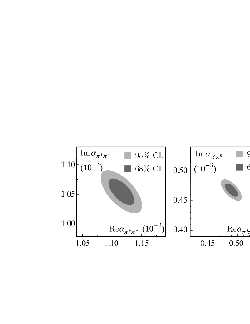
Figure 1: Representation of $\alpha_{\pi^{+}\pi^{-}}$ and $\alpha_{\pi^{0}\pi^{0}}$ in the complex plane. In each case, the two ellipses represent the 68% and the 95% CL contours.

Following the discussion in section 2.1, we determine $\alpha_{\pi^{+}\pi^{-}\gamma_{\rm DE}}$ from the measurement of $\eta_{+-\gamma}$ from Ref. [17] and BR$(K_{S}\rightarrow\pi^{+}\pi^{-}\gamma)$ from the measurement of $R_{S,\gamma}={\rm BR}(K_{S}\rightarrow\pi^{+}\pi^{-}\gamma)/{\rm BR}(K_{S}\rightarrow\pi^{+}\pi^{-})$  [18]. The photon energy threshold was 20 MeV for both measurements. The value of $R_{S,\gamma}^{\rm th-IB}=\left(\vphantom{H^{I}_{I}}{\rm BR}(K_{S}\rightarrow\pi\pi\gamma)/{\rm BR}(K_{S}\rightarrow\pi\pi)\right)^{\rm th-IB}=(0.700\pm 0.001)\times 10^{-2}$ is calculated using the KLOE MC generator, which is described in Ref. 19. Figure 2(a) shows the 68% and the 95% CL contours for $\alpha_{\pi^{+}\pi^{-}\gamma_{DE}}$. We find a very small contribution:

$$\alpha_{\pi^{+}\pi^{-}\gamma_{DE}}=\left(\vphantom{H^{I}_{I}}(5\pm 7)+i(6\pm 7)\right)\times 10^{-7}\,.$$

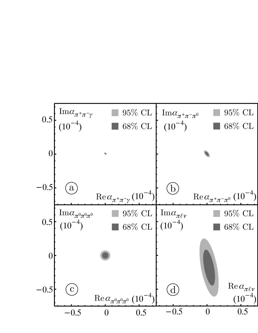
Figure 2: Bounds of the $\alpha$ values for three-body decays of $K_{S}$, $K_{L}$. Note that the same scale is used for all plots.

3.2 Three-pion modes

Until the recent results from KLOE [5] and NA48 [8] became available, the limiting contribution to the $CPT$ test was due to the $3\pi^{0}$ final state. The upper limit on $|\alpha_{\pi^{0}\pi^{0}\pi^{0}}|$ is evaluated from eq. (12) using the KLOE upper limit BR($K_{S}$$\rightarrow$3$\pi^{0}$)$<1.5\times 10^{-7}$ at 95% CL [5] and the value of BR($K_{L}$$\rightarrow$3$\pi^{0}$) from the KLOE average. The phase $\phi_{000}$ is taken as uniform in $\{0,2\pi\}$. For $\alpha_{\pi^{+}\pi^{-}\pi^{0}}$, eq. (10), we use ${\rm Re}(\eta_{+-0})$ and ${\rm Im}(\eta_{+-0})$ as measured by CPLEAR [10] and the value of BR($K_{L}$$\rightarrow$$\pi^{+}\pi^{-}$$\pi^{0}$) from the KLOE average, all given in table 1.

The 68% and the 95% CL contours for $\alpha_{\pi^{+}\pi^{-}\pi^{0}}$, and the 95% CL contour for $\alpha_{\pi^{0}\pi^{0}\pi^{0}}$ are shown in figures 2(b) and 2(c), respectively. We find:

$$\alpha_{\pi^{+}\pi^{-}\pi^{0}} = \left(\vphantom{H^{I}_{I}}(0\pm 2)+i(0\pm 2)\right)\times 10^{-6},$$

$$|\alpha_{\pi^{0}\pi^{0}\pi^{0}}| < 7\times 10^{-6}{\rm~{}~{}at~{}95\%~{}CL}\,.$$

3.3 Semileptonic modes

For the determination of $\alpha_{\pi\ell\nu}$ from eq. (15), we combine the KLOE measurement [6] of the $K_{S}$ semileptonic charge asymmetry $A_{S}$ for $K_{S}$  semileptonic decays, the PDG average [14] for $K_{L}$  semileptonic charge asymmetry $A_{L}$, and the CPLEAR time-dependent measurement of $K^{0}\vphantom{\overline{K}{}^{0}}$and $\overline{K}{}^{0}$  semileptonic rates [13]. The original CPLEAR result is given in table 3.

	value	Correlation coefficients
${\rm Re}(\delta)$	$(3.0\pm 3.4)\times 10^{-4}$	1
${\rm Im}(\delta)$	$(-1.5\pm 2.3)\times 10^{-2}$	0.44	1
${\rm Re}(x_{-})$	$(0.2\pm 1.3)\times 10^{-2}$	-0.56	-0.97	1
${\rm Im}(x_{+})$	$(1.2\pm 2.2)\times 10^{-2}$	-0.60	-0.91	0.96	1

Table 3: Values, errors, and correlation coefficients for ${\rm Re}(\delta)$, ${\rm Im}(\delta)$, ${\rm Re}(x_{-})$, and ${\rm Im}(x_{+})$ measured by CPLEAR.

We have improved this result by adding the measurement of $A_{S}-A_{L}=4[{\rm Re}(\delta)+{\rm Re}(x_{-})]=(-2\pm 10)\times 10^{-3}$ [6, 14]. The results, referred to as the $K_{\ell 3}$ average, are given in table 4.

	value	Correlation coefficients
${\rm Re}(\delta)$	$(3.4\pm 2.8)\times 10^{-4}$	1
${\rm Im}(\delta)$	$(-1.0\pm 0.7)\times 10^{-2}$	-0.27	1
${\rm Re}(x_{-})$	$(-0.07\pm 0.25)\times 10^{-2}$	-0.23	-0.58	1
${\rm Im}(x_{+})$	$(0.8\pm 0.7)\times 10^{-2}$	-0.35	-0.12	0.57	1
$A_{S}+A_{L}$	$(0.5\pm 1.0)\times 10^{-2}$	-0.12	-0.62	0.99	0.54	1

Table 4: Values, errors, and correlation coefficients for ${\rm Re}(\delta)$, ${\rm Im}(\delta)$, ${\rm Re}(x_{-})$, ${\rm Im}(x_{+})$, and $A_{S}+A_{L}$ obtained from a combined fit ($K_{\ell 3}$ average).

Finally, for ${\rm BR}(K_{L}\rightarrow\pi\ell\nu)$ we use the sum of $K_{e3}$ and $K_{\mu 3}$ branching ratios from the KLOE average. Figure 2(d) shows the 68% and the 95% CL contours for $\alpha_{\pi\ell\nu}$. We find:

$$\alpha_{\pi\ell\nu}=\left(\vphantom{H^{I}_{I}}(0.3\pm 0.6)+i(-1.8\pm 1.8)\right)\times 10^{-5}\,.$$

4 Results

Inserting the values of the $\alpha$ parameters into eq. (16), we obtain :

$${\rm Re}(\epsilon)=(159.6\pm 1.3)\times 10^{-5},\qquad{\rm Im}(\delta)=(0.4\pm 2.1)\times 10^{-5}\,,$$ (18)

where all correlations among the input data are taken into account, including that from the direct determination of ${\rm Im}(\delta)$ from the semileptonic decays. The complete information is given in table 5.

	value	Correlation coefficients
${\rm Re}(\epsilon)$	$(159.6\pm 1.3)\times 10^{-5}$	1
${\rm Im}(\delta)$	$(0.4\pm 2.1)\times 10^{-5}$	-0.17	1
${\rm Re}(\delta)$	$(2.3\pm 2.7)\times 10^{-4}$	0.20	-0.22	1
${\rm Re}(x_{-})$	$(-2.9\pm 2.0)\times 10^{-3}$	-0.25	0.37	-0.49	1

Table 5: Summary of results: values, errors, and correlation coefficients for ${\rm Re}(\epsilon)$, ${\rm Im}(\delta)$, ${\rm Re}(\delta)$, and ${\rm Re}(x_{-})$.

The allowed region in the ${\rm Re}(\epsilon)$, ${\rm Im}(\delta)$ plane at 68% CL and 95% CL is shown in the left panel of figure 3.

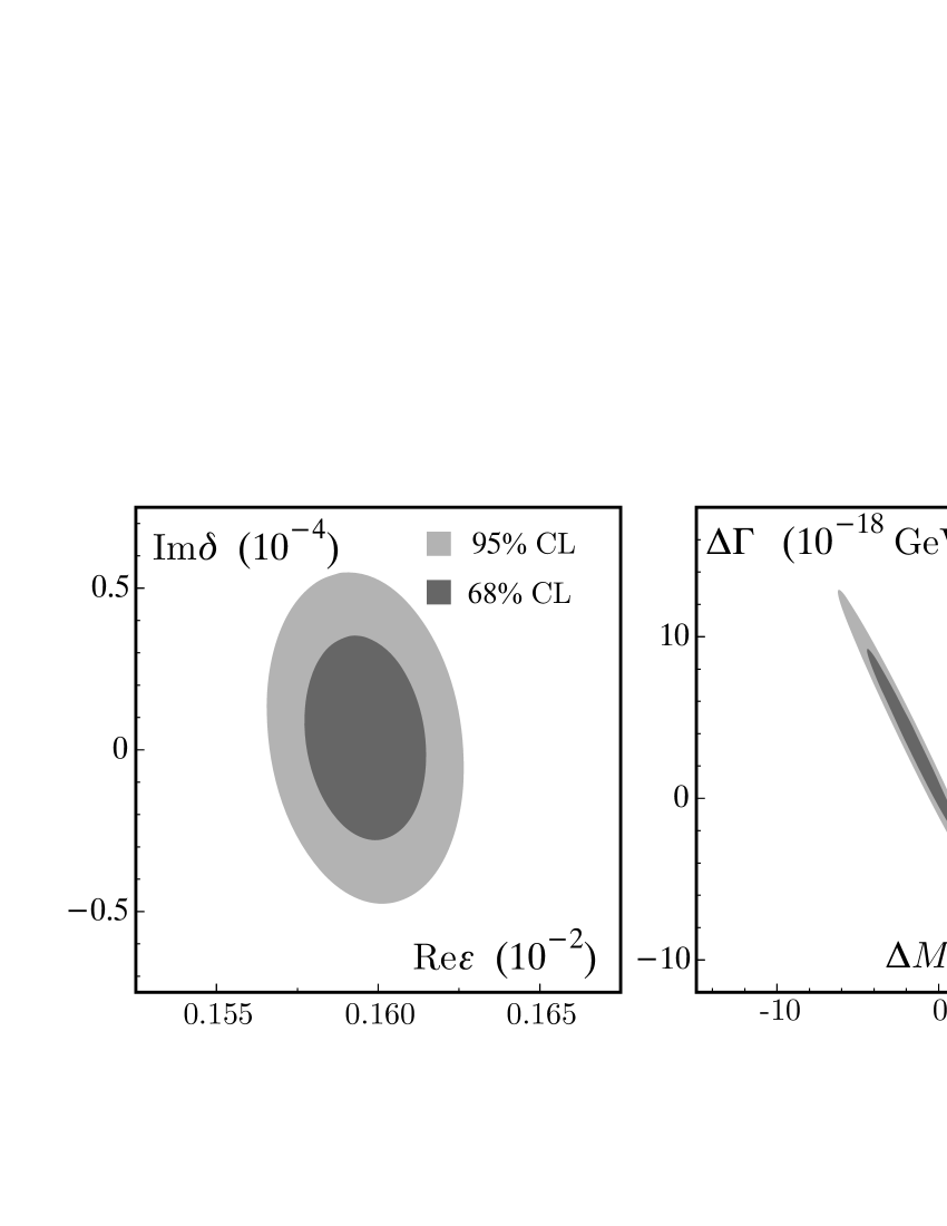
Figure 3: Left: allowed region at 68% and 95% CL in the ${\rm Re}(\epsilon)$, ${\rm Im}(\delta)$ plane. Right: allowed region at 68% and 95% CL in the $\Delta M,\Delta\Gamma$ plane.

A small correlation between ${\rm Re}(\epsilon)$ and ${\rm Im}(\delta)$ is evident, which is due to the semileptonic term. With the new KLOE data used in the present analysis, the process giving the largest contribution to the size of the allowed region is now $K_{L}\rightarrow\pi^{+}\pi^{-}$, through the uncertainty on $\phi_{+-}$. Besides the $\pi\pi$ final states, only the semileptonic term gives an appreciable contribution ($\sim 10\%$) to the error on ${\rm Im}(\delta)$. Our results, Eq. 18, are a significant improvement over those of CPLEAR [7]:

$${\rm Re}(\epsilon)=(164.9\pm 2.5)\times 10^{-5},\qquad{\rm Im}(\delta)=(2.4\pm 5.0)\times 10^{-5}.$$

Note also that the central value of ${\rm Re}(\epsilon)$ is quite different. This is due to the new measurement of BR($K_{L}$$\rightarrow$$\pi^{+}\pi^{-}$) [4].

The limits on ${\rm Im}(\delta)$ and ${\rm Re}(\delta)$ can be used to constrain the mass and width difference between $K^{0}\vphantom{\overline{K}{}^{0}}$ and $\overline{K}{}^{0}$ via

$$\delta={{i(m_{K^{0}\vphantom{\overline{K}{}^{0}}}-m_{\overline{K}{}^{0}})+{1\over 2}(\Gamma_{K^{0}\vphantom{\overline{K}{}^{0}}}-\Gamma_{\overline{K}{}^{0}})}\over{\Gamma_{S}-\Gamma_{L}}}\cos\phi_{SW}e^{i\phi_{SW}}[1+{\mathcal{O}}(\epsilon)]\,.$$

The allowed region in the $\Delta M=(m_{K^{0}\vphantom{\overline{K}{}^{0}}}-m_{\overline{K}{}^{0}}),\Delta\Gamma=(\Gamma_{K^{0}\vphantom{\overline{K}{}^{0}}}-\Gamma_{\overline{K}{}^{0}})$ plane is shown in the right panel of figure 3. The strong correlation reflects the high precision of ${\rm Im}(\delta)$ compared to ${\rm Re}(\delta)$. Since the total decay widths are dominated by long-distance dynamics, in models where $CPT$ invariance is a pure short-distance phenomenon, it is useful to consider the limit $\Gamma_{K^{0}\vphantom{\overline{K}{}^{0}}}=\Gamma_{\overline{K}{}^{0}}$. In this limit (i.e. neglecting $CPT$-violating effects in the decay amplitudes), we obtain the following bound on the neutral kaon mass difference:

$$-5.3\times 10^{-19}~{}{\rm GeV}<m_{K^{0}\vphantom{\overline{K}{}^{0}}}-m_{\overline{K}{}^{0}}<6.3\times 10^{-19}~{}\rm{GeV\quad at~{}95~{}\%~{}CL}\,.$$

Our result represents a significant improvement with respect to $|m_{K^{0}\vphantom{\overline{K}{}^{0}}}-m_{\overline{K}{}^{0}}|<12.7\times 10^{-19}~{}{\rm GeV}$ at 90% CL, obtained by CPLEAR [10].

Appendix A The $\pi\pi\gamma$ contribution to the $\alpha_{i}$

By construction, the leading contribution of the $\pi\pi\gamma$ state to the unitarity sum, namely the interference of the $K_{L}$ and $K_{S}$ bremsstrahlung amplitudes, is included in $\alpha_{+-(\gamma)}$. The largest sub-leading term missing in $\alpha_{+-(\gamma)}$ is the DE-bremsstrahlung interference, which we include in $\alpha_{\pi\pi\gamma_{\rm E1-S(L)}}$ of eq. (8). To evaluate this contribution, we introduce the total (IB+DE) amplitude ratio

$$\eta_{+-\gamma}(E_{\gamma})=\frac{\mathcal{A}_{L}(\pi\pi\gamma_{\rm IB+E1})}{\mathcal{A}_{S}(\pi\pi\gamma_{\rm IB+E1})}=\eta_{+-}+\epsilon^{\,\prime}_{+-\gamma}(E_{\gamma})$$ (19)

This ratio is an observable quantity which can be measured in an interference experiment [17]. As explicitly indicated, $\eta_{+-\gamma}$ depends on the photon energy and it can be decomposed into the energy-independent parameter $\eta_{+-}$ and the direct-$CP$-violating term $\epsilon^{\,\prime}_{+-\gamma}$. In the $E_{\gamma}\rightarrow 0$ limit $\epsilon^{\,\prime}_{+-\gamma}\propto E_{\gamma}^{2}$ [11]. Using eq. (19), we can write

$$\frac{1}{\Gamma_{S}}\left\langle\vphantom{H^{I}_{I}}\mathcal{A}_{L}(\pi\pi\gamma)\mathcal{A}^{*}_{S}(\pi\pi\gamma_{\rm E1})+\mathcal{A}_{L}(\pi\pi\gamma_{\rm E1})\mathcal{A}^{*}_{S}(\pi\pi\gamma)\right\rangle=$$

$$=\frac{1}{\Gamma_{S}}\left\langle\vphantom{H^{I}_{I}}\>\eta_{+-}\>\left(\vphantom{H^{I}_{I}}\mathcal{A}_{S}(\pi\pi\gamma)\mathcal{A}^{*}_{S}(\pi\pi\gamma_{\rm E1})+\mathcal{A}_{S}(\pi\pi\gamma_{\rm E1})\mathcal{A}^{*}_{S}(\pi\pi\gamma)\right)+\right.$$

$$\qquad\quad\left.+\epsilon^{\,\prime}_{+-\gamma}~{}\mathcal{A}_{S}(\pi\pi\gamma)\mathcal{A}^{*}_{S}(\pi\pi\gamma)(1+\delta_{\rm E1})\right\rangle$$

$$\approx~{}\eta_{+-}~{}\Delta B(K_{S}\rightarrow\pi\pi\gamma_{\rm DE})+\frac{1}{\Gamma_{S}}\int dE_{\gamma}~{}\epsilon^{\,\prime}_{+-\gamma}~{}\frac{d\Gamma(K_{S}\rightarrow\pi\pi\gamma)}{dE_{\gamma}}$$ (20)

where $\delta_{\rm E1}=\mathcal{A}_{S}(\pi\pi\gamma_{\rm E1})/\mathcal{A}_{S}(\pi\pi\gamma)$ is a very small overall correction factor which can be safely neglected and $\Delta B(K_{S}\rightarrow\pi\pi\gamma_{\rm DE})={\rm BR}(K_{S}\rightarrow\pi\pi\gamma)^{\rm exp}-{\rm BR}(K_{S}\rightarrow\pi\pi\gamma)^{\rm th-IB}$ is the deviation of the observed $K_{S}\rightarrow\pi\pi\gamma$ decay rate from that inferred from a pure bremsstrahlung spectrum. By construction, the integral on the right-hand side of eq. (20) is infrared safe. Since at present there is no evidence for a non-vanishing $\epsilon{\,{}^{\prime}}_{+-\gamma}$ [17], in eq. (9) we replace this integral with the product $(\eta_{+-\gamma}-\eta_{+-})\times{\rm BR}(K_{S}\rightarrow\pi\pi\gamma)$, where ${\rm BR}(K_{S}\rightarrow\pi\pi\gamma)$ indicates the branching fraction for a real photon emission with minimum photon-energy cut equivalent to that used in the corresponding $\eta_{+-\gamma}$ measurement ($E^{\rm cut}_{\gamma}=$ 20 MeV in Ref. 17). The contribution to eq. (20) generated by $K_{L,S}\rightarrow\pi\pi\gamma$ amplitudes with $E_{\gamma}<E^{\rm cut}_{\gamma}$ vanishes in the limit $E_{\gamma}^{\rm cut}\rightarrow 0$ and can be safely neglected.

References

- [1] G. Lüders, Ann. Phys. 2 (1957) 1, reprinted in Ann. Phys. 281 (2000) 1004.
- [2] See e.g. J. Bernabeu, J. Ellis, N. E. Mavromatos, D. V. Nanopoulos and J. Papavassiliou, hep-ph/0607322; V.A. Kostelecky and R. Lehnert, Phys. Rev. D 63 (2001) 065008; and references therein.
- [3] J.S. Bell and J. Steinberger, Proceedings Oxford Int. Conf. on Elementary Particles (1965).
- [4] KLOE Collaboration, F. Ambrosino et al., Phys. Lett. B 638 (2006) 140.
- [5] KLOE Collaboration, F. Ambrosino et al., Phys. Lett. B 619 (2005) 61.
- [6] KLOE Collaboration, F. Ambrosino et al., Phys. Lett. B 636 (2006) 173.
- [7] CPLEAR Collaboration, A. Apostolakis et al., Phys. Lett. B 456 (1999) 297.
- [8] NA48 Collaboration, A. Lai et al., Phys. Lett. B 610 (2005) 165.
-
[9]
V. Weisskopf and E.P. Wigner, Z. Phys. 63 (1930) 54;
T.D. Lee, R. Oehme and C.N. Yang, Phys. Rev. 106 (1957) 340. - [10] CPLEAR Collaboration, A. Angelopoulos et al., Phys. Rept. 374 (2003) 165.
- [11] G. D’Ambrosio and G. Isidori, Int. J. Mod. Phys. A 13 (1998) 1.
- [12] L. Maiani, G. Pancheri and N. Paver, The Second DANE Physics Handbook (Frascati, 1995).
- [13] CPLEAR Collaboration, A. Angelopoulos et al., Eur. Phys. J. C 22 (2001) 55.
- [14] Particle Data Group, W.-M. Yao et al., J. Phys. G 33 (2006) 1.
- [15] KTeV Collaboration,T. Alexopoulos et al., Phys. Rev. D 70 (2004) 092006.
- [16] KLOE Collaboration,hep-ex/0601025, accepted by Eur. Phys. J. C.
- [17] J. N. Matthews et al., Phys. Rev. Lett. 75 (1995) 2806.
- [18] E. Ramberg et al., Phys. Rev. Lett. 70 (1993) 2525.
- [19] C. Gatti, Eur. Phys. J. C 45 (2005) 417; and references therein.
- [20] KLOE Collaboration, F. Ambrosino et al., Phys. Lett. B 626 (2005) 15.
- [21] KLOE Collaboration, F. Ambrosino et al., Phys. Lett. B 632 (2006) 43.
- [22] NA48 Collaboration, A. Lai et al., Phys. Lett. B 602 (2004) 41.
- [23] K.G. Vosburgh et al., Phys. Rev. D 6 (1972) 1834.