DEMO-HEP 97/09 20 November, 1997

Accurate Estimation of the Trilinear Gauge Couplings Using Optimal Observables Including Detector Effects

G. K. Fanourakis, D. Fassouliotis and S. E. Tzamarias

N.C.S.R. Demokritos

This paper describes the definition of maximum likelihood equivalent estimators of the Trilinear Gauge Couplings which include detector effects. The asymptotic properties of these estimators as well as their unbiasedness and efficiency when dealing with finite statistical samples are demonstrated by Monte Carlo experimentation, using simulated events corresponding to the reaction $e^{+}e^{-}\rightarrow q\bar{q}l\nu$ at 172 GeV. Emphasis is given to the determination of the expected efficiencies in extracting the $\alpha_{W\phi}$, $\alpha_{W}$ and $\alpha_{B\phi}$ couplings from LEPII data, which in this particular case found to be close to the maximum possible.

1 Introduction

It has been often emphasized that the likelihood estimators can reach the lower bound of the Cramer-Rao [1] inequality,

$$V(\hat{\lambda})\geq[-E(\frac{\partial^{2}\ln{L}}{\partial\lambda^{2}})_{\lambda=\hat{\lambda}}]^{-1}\geq\frac{-1}{{\cal{I}}_{\lambda}}$$ (1)

where:

$\hat{\lambda}$

is the likelihood estimation of a parameter $\lambda$

$L$

is the likelihood function

$V$

and $E$ are the variance and expected value operators respectively

$\cal{I}_{\lambda}$

denotes the maximum available information with respect to $\lambda$.

The right hand side bound depends on the construction of the probability density function (p.d.f.). Thus, as has been shown in [2] and [3], in order to reach the maximum accuracy in estimating the Trilinear Gauge Couplings, the complete kinematical information has to be included in $L$. However, when the measured kinematic vectors are used, the experimental uncertainties must be explicitly taken into account in the p.d.f. formulation. In other words, the data must be compared with the distribution:

$$P(\vec{\Omega};\vec{\lambda})=\int g(\vec{V};\vec{\lambda})\cdot R(\vec{V},\vec{\Omega})d\vec{V}$$ (2)

rather than with

$$g(\vec{V};\vec{\lambda})=\frac{(d\sigma(\vec{V};\vec{\lambda})/d\vec{V})\cdot\epsilon(\vec{V})}{\sigma_{obs.}(\vec{\lambda})}$$ (3)

where

$\vec{V}=\{V_{1},\ldots,V_{m}\}$ and $\vec{\Omega}=\{\Omega_{1},\ldots,\Omega_{m}\}$ are the true and measured m-dimensional kinematic vectors respectively.

$\vec{\lambda}$

is the set of $\rho$ physics parameters $\{\lambda_{1},\ldots,\lambda_{\rho}\}$ which are needed to define completely the p.d.f.

$\epsilon(\vec{V})$

is the selection efficiency function taking values continuously between zero and one,

$d\sigma(\vec{V};\vec{\lambda})/d\vec{V}$

is the differential cross section.

$\sigma_{obs.}(\vec{\lambda})$

is the total observed cross section defined as:

$$\sigma_{obs.}(\vec{\lambda})=\int(d\sigma(\vec{V};\vec{\lambda})/d\vec{V})\cdot\epsilon(\vec{V})d\vec{V}$$ (4)

$R(\vec{V},\vec{\Omega})$

is the resolution function, or else the probability for the true kinematic vector $\vec{V}$ of an event to be measured as $\vec{\Omega}$.

$g(\vec{V};\vec{\lambda})$

is the p.d.f. according to which the vectors $\vec{V}$ are distributed and

$P(\vec{\Omega};\vec{\lambda})$

is the p.d.f. according to which the vectors $\vec{\Omega}$ are distributed.

The use of (2), in multi-dimensional phase space, faces several difficulties of which the parameterization of the resolution functions is the most serious. The often offered remedies consist of either using (3) instead of (2) with the hope that possible biases will be determined afterwards by Monte Carlo (M.C.) experimentation or of integrating over some of the kinematic variables and paramererizing the resolution with respect to the remaining fewer kinematic components.

This paper concentrates on the definition of likelihood equivalent estimators which, whilst including the description of all the detector effects, retain the maximum likelihood sensitivity in extracting the values of the Trilinear Gauge Couplings. The next Section briefly describes the topological and kinematic features of the data samples used in this analysis. In Section 3, ways of reducing the number of the necessary kinematic variables are discussed when the detector effects are negligible. In Section 4 the results obtained in the ideal case are extrapolated to the case when the detector effects are important. A demonstration of the optimal properties of the proposed techniques is given at Section 5 by Monte Carlo experimentation. Finally, Section 6 compiles the conclusions of this analysis.

2 The Four-Fermion Semileptonic Final States

One of the important physics issues of the LEPII program is the determination of the non-Abelian self couplings ( Trilinear Gauge Couplings, in the following TGC’s) of the carriers of the electroweak interaction. The measurement of the WWV couplings, where W stands for the W gauge boson whilst V denotes the $\gamma$ or $Z^{0}$ neutral carriers, is possible via WW production [3] through diagrams involving exchange of $Z^{0}$ and $\gamma$. Limiting the phenomenological analysis to the contribution of gauge invariant operators of dimension less than six [4], there are 3 CP conserving ($\alpha_{W\phi}$, $\alpha_{W}$ and $\alpha_{B\phi}$) and 2 CP violating ($\tilde{\alpha}_{BW}$ and $\tilde{\alpha}_{W}$) couplings which by deviating from their Standard Model values, could point to the existence of new physics.

Several final state topologies, corresponding to the production of a pair or of a single W and to the different W decay modes, can be used to determine the TGC’s. In this paper only final states including a charged lepton, two hadronic jets and an invisible neutrino are considered. These final states, in the following semileptonic final states, suffer less from kinematic ambiguities and consequently a more precise measurement can be made.

However, W pair production diagrams alone are not sufficient to express the production dynamics of the semileptonic states [3]. Throughout this paper full four-fermion phenomenological models including Coulomb corrections and Initial State Radiation (ISR) [5],[6] are used to describe the kinematic distributions and/or to produce Monte Carlo events as functions of the CP conserving couplings.

The detector simulation program DELSIM [7] was used to study the effect of the distortion of the kinematic distributions, due to the event selection efficiency and the detector resolution, on the measurement of the TGC’s. Special care was taken in selecting the semileptonic four fermion final state topologies in order to avoid contamination from products irrelevant to the determination of the TGCs. The selection criteria, based on the lepton identification jet reconstruction and missing visible energy, are discussed in details in [8]. An improvement in the measurement accuracy of the kinematic vectors was achieved by a six-constraint kinematic fit.

After the constrained fit, all the eight kinematic variables needed to specify an event completely were determined up to a degeneracy in the charge of the hadronic jets. The latter resulted in a loss of information by averaging the squared matrix elements corresponding to the two momentum assignments [2] [3].

3 The Ideal Case

The differential cross section is parameterized as a quadratic function of the TGC’s [3] of the form:

$$d\sigma(\vec{V};\vec{\lambda})/d\vec{V}=c_{0}(\vec{V})+\sum_{k}c^{k}_{1}(\vec{V})\cdot\lambda_{k}+\sum_{\mu,k}c_{2}^{\mu k}(\vec{V})\cdot\lambda_{\mu}\cdot\lambda_{k}$$ (5)

where the vector $\vec{V}$ is of dimension eight and $\vec{\lambda}=\{\lambda_{1},\ldots,\lambda_{\rho}\}$ is the set of the TGC’s which are allowed to deviate from their Standard Model (S.M.) values. Following eq. (4), the total cross section can be expressed as:

$$\sigma_{tot}(\vec{\lambda})=S_{0}+\sum_{k}S_{1}^{k}\cdot\lambda_{k}+\sum_{\mu k}S_{2}^{\mu k}\cdot\lambda_{\mu}\cdot\lambda_{k}$$ (6)

$$S_{i}^{j}=\int c_{i}^{j}(\vec{V})d\vec{V}$$ (7)

When the detector effects are negligible the p.d.f. takes the form:

$$g(\vec{V},\vec{\lambda})=\frac{c_{0}(\vec{V})+\sum_{k}c^{k}_{1}(\vec{V})\cdot\lambda_{k}+\sum_{\mu,k}c_{2}^{\mu k}(\vec{V})\cdot\lambda_{\mu}\cdot\lambda_{k}}{S_{0}+\sum_{k}S_{1}^{k}\cdot\lambda_{k}+\sum_{\mu k}S_{2}^{\mu k}\cdot\lambda_{\mu}\cdot\lambda_{k}}$$ (8)

and the likelihood function for a set of N observed events with kinematic vectors $\vec{V}_{n}$, $n=1,\ldots,N$ is defined as:

$$L(\vec{V}_{1},\ldots,\vec{V}_{N};\vec{\lambda})=\prod_{n=1}^{N}g(\vec{V}_{n},\vec{\lambda})$$ (9)

3.1 Optimal Variables

The kinematic distribution with respect to a subset of the components of $\vec{V}$, let’s say $X=\{V_{1},\ldots,V_{\nu}\}$ with $\nu<m$, is found by integrating (8) as:

$$\varpi(q_{1},\ldots,q_{\nu};\vec{\lambda})=\int g(\vec{V};\vec{\lambda})\cdot\delta(q_{1}-V_{1})\cdots\delta(q_{\nu}-V_{\nu})dV_{1}\cdots dV_{\nu}\cdots dV_{m}$$ (10)

and the corresponding likelihood function for N events is:

$$L(X_{1},\ldots,X_{N};\vec{\lambda})=\prod_{n=1}^{N}\varpi(X_{n};\vec{\lambda})$$ (11)

The likelihood estimators of the couplings $\vec{\lambda}$ are defined as the solutions of the following system of equations :

$$\int[\frac{\partial\ln{L(X_{1},\ldots,X_{N};\vec{\lambda})}}{\partial\lambda_{j}}]_{\vec{\lambda}=\hat{\lambda}}\cdot L(X_{1},\ldots,X_{N};\vec{\lambda}=\vec{\lambda}_{true})dX_{1}\cdots dX_{N}=0$$ (12)

or equivalently [1]

$$N\cdot\int[\frac{\partial\ln{\varpi(X;\vec{\lambda})}}{\partial\lambda_{j}}]_{\vec{\lambda}=\hat{\lambda}}\cdot\varpi(X;\vec{\lambda}=\vec{\lambda}_{true})dX=0$$ (13)

where $\vec{\lambda}_{true}$, $\hat{\lambda}$ are the true and the estimated values of the couplings respectively. If a single set of N observed events is available eq. (13) is approximated as:

$$\frac{\partial\ln{L(X_{1},\ldots,X_{N};\vec{\lambda})}}{\partial\lambda_{j}}]_{\vec{\lambda}=\hat{\lambda}}=\sum_{k=1}^{N}\frac{\partial\ln{\varpi(X_{k};\vec{\lambda})}}{\partial\lambda_{j}}]_{\vec{\lambda}=\hat{\lambda}}=0$$ (14)

The maximum likelihood estimation (14) satisfies at the asymptotic limit the left side bound of (1). However, the right side bound of the Cramer-Rao inequality is not necessarily satisfied after projecting the p.d.f. Indeed, in [2] and [3] traditional kinematic distributions such as the W production angle, the charged lepton angle with respect to the W direction in the W rest frame etc. have been rated according to their efficiency in estimating the TGC’s and they have been found inferior to the eight-fold unbinned likelihood fit.

Searching for a subset of the kinematic components which contain all the available information with respect to $\vec{\lambda}$, one has to start from the error matrix of the likelihood estimators when all the kinematic variables have been used, as in (8) and (9). In the asymptotic limit this matrix has elements given by (1), i.e.:

$$V(\lambda_{i},\lambda_{j}) = [-E(\frac{\partial^{2}\ln{L(\vec{V}_{1},\ldots,\vec{V}_{N};\vec{\lambda}=\hat{\lambda})}}{\partial\lambda_{i}\partial\lambda_{j}})]^{-1}$$ (15)

$$= \frac{-1}{N}\cdot[\int\frac{\partial^{2}\ln{g(\vec{V};\vec{\lambda}=\hat{\lambda})}}{\partial\lambda_{i}\partial\lambda_{j}}g(\vec{V};\vec{\lambda}=\vec{\lambda}_{true})d\vec{V}]^{-1}$$

The second derivative in (15) depends on the kinematic vectors $\vec{V}$ through terms such as $c_{1}^{k}(\vec{V})/c_{0}(\vec{V})$ and $c_{2}^{\mu k}(\vec{V})/c_{0}(\vec{V})$. This has significant implications especially when only one parameter TGC models are used. In this case the p.d.f. is written as:

$$g(\vec{V};\lambda)=\frac{c_{0}(\vec{V})+c_{1}(\vec{V})\cdot\lambda+c_{2}(\vec{V})\cdot\lambda^{2}}{S_{0}+S_{1}\cdot\lambda+S_{2}\cdot\lambda^{2}}$$ (16)

where the terms $c_{0}(\vec{V})$, $c_{1}(\vec{V})$ and $c_{2}(\vec{V})$ correspond to the particular choice of the TGC $\lambda$.
The error in the maximum likelihood estimation of $\hat{\lambda}$ will be:

$$V(\hat{\lambda})= \frac{-1}{N}\cdot[-\frac{2\cdot S_{2}\cdot(S_{0}+S_{1}\cdot\hat{\lambda}+S_{2}\cdot\hat{\lambda}^{2})-(S_{1}+2\cdot S_{2}\cdot\hat{\lambda})^{2}}{(S_{0}+S_{1}\cdot\hat{\lambda}+S_{2}\cdot\hat{\lambda}^{2})^{2}}$$ (17)

$$+\int\frac{2\cdot Q_{2}(\vec{V})\cdot(1+Q_{1}(\vec{V})\cdot\hat{\lambda}+Q_{2}(\vec{V})\cdot\hat{\lambda}^{2})-(Q_{1}(\vec{V})+2\cdot Q_{2}(\vec{V})\cdot\hat{\lambda})^{2}}{(1+Q_{1}(\vec{V})\cdot\hat{\lambda}+Q_{2}(\vec{V})\cdot\hat{\lambda}^{2})^{2}}$$

$$\cdot g(\vec{V};\lambda_{true})d\vec{V}]^{-1}$$

where

$$Q_{1}(\vec{V})=\frac{c_{1}(\vec{V})}{c_{0}(\vec{V})}$$ (18)

$$Q_{2}(\vec{V})=\frac{c_{2}(\vec{V})}{c_{0}(\vec{V})}$$ (19)

However, when the likelihood function is expressed in terms of the projected probability distribution:

$${\varpi}(q_{1},q_{2};\lambda)=\int g(\vec{V};\lambda)\cdot\delta(q_{1}-Q_{1}(\vec{V}))\cdot\delta(q_{2}-Q_{2}(\vec{V}))d\vec{V}$$ (20)

the variance of the estimated coupling will be:

$$V(\hat{\lambda})= \frac{-1}{N}\cdot[-\frac{2\cdot S_{2}\cdot(S_{0}+S_{1}\cdot\hat{\lambda}+S_{2}\cdot\hat{\lambda}^{2})-(S_{1}+2\cdot S_{2}\cdot\hat{\lambda})^{2}}{(S_{0}+S_{1}\cdot\hat{\lambda}+S_{2}\cdot\hat{\lambda}^{2})^{2}}$$ (21)

$$+\int\int\int\{\frac{2\cdot q_{2}\cdot(1+q_{1}\cdot\hat{\lambda}+q_{2}\cdot\hat{\lambda}^{2})-(q_{1}+2\cdot q_{2}\cdot\hat{\lambda})^{2}}{(1+q_{1}\cdot\hat{\lambda}+q_{2}\cdot\hat{\lambda}^{2})^{2}}$$

$$\cdot g(\vec{V};\lambda_{true})\cdot\delta(q_{1}-Q_{1}(\vec{V}))\cdot\delta(q_{2}-Q_{2}(\vec{V}))\}d\vec{V}dq_{1}dq_{2}]^{-1}$$

Reversing the order of integration in (21) and integrating first with respect to $q_{1}$ and $q_{2}$ it is easy to see that the achieved accuracy by employing the projected distribution (20) is the same as when the complete multi-dimensional distribution (16) is used.

3.2 The Optimal Observables

The reduction of the number of necessary kinematic components is not so dramatic when more than one TGC are to be simultaneously extracted from the data. There is, though, the possibility of a further reduction in the number of the necessary kinematic variables by expanding the p.d.f. in a Taylor series and keeping only the linear terms. Returning to the general case of estimating simultaneously $\rho$ couplings, the distribution function (8) is approximated in the neighborhood of the expansion point $\lambda^{0}$ as:

$$g(\vec{V};\vec{\lambda})\simeq\frac{y_{0}(\vec{V};\vec{\lambda}^{0})}{Z_{0}(\vec{\lambda}^{0})}\cdot[1+\sum_{k=1}^{\rho}(\frac{y_{1}^{k}(\vec{V};\vec{\lambda}^{0})}{y_{0}(\vec{V};\vec{\lambda}^{0})}-\frac{Z_{1}^{k}(\vec{\lambda}^{0})}{Z_{0}(\vec{\lambda}^{0})})\cdot\Delta_{k}]$$ (22)

where

$$y_{0}(\vec{V};\vec{\lambda}^{0})=c_{0}(\vec{V})+\sum_{k}C_{1}^{k}(\vec{V})\cdot{\lambda}^{0}_{k}+\sum_{\mu k}c_{2}^{\mu k}(\vec{V})\cdot{\lambda}^{0}_{\mu}\cdot{\lambda}^{0}_{k}$$ (23)

$$y_{1}^{k}(\vec{V};\vec{\lambda}^{0})=c_{1}^{k}(\vec{V})+\sum_{\mu}C_{2}^{\mu k}(\vec{V})\cdot{\lambda}^{0}_{\mu}$$ (24)

$$Z_{\rho}^{k}=\int y_{\rho}^{k}d\vec{V}$$ (25)

and $\Delta_{k}={\lambda}_{k}-{\lambda}^{0}_{k}$.

Furthermore, by projecting (22) as:

$$\varpi(O_{1}(\vec{\lambda}^{0}),\ldots,O_{\rho}(\vec{\lambda}^{0});\vec{\lambda})=$$

$$\int g(\vec{V};\vec{\lambda})\cdot\delta(O_{1}(\vec{\lambda}^{0})-\frac{y_{1}^{1}(\vec{V};\vec{\lambda}^{0})}{y_{0}(\vec{V};\vec{\lambda}^{0})})\cdots\delta(O_{\rho}(\vec{\lambda}^{0})-\frac{y_{1}^{k}(\vec{V};\vec{\lambda}^{0})}{y_{0}(\vec{V};\vec{\lambda}^{0})})d\vec{V}$$ (26)

the number of the necessary kinematic variables are reduced to as many as the number of parameters to be fitted simultaneously without losing information. It has been also shown in [9] that there are simple statistics equivalent to the maximum likelihood estimators. These are the mean values of $O_{k}(\vec{V},\vec{\lambda}^{0})$ , called Optimal Observables, defined as:

$$O_{k}(\vec{V};\vec{\lambda}^{0})=\frac{y_{1}^{k}(\vec{V};\vec{\lambda}^{0})}{y_{0}(\vec{V};\vec{\lambda}^{0})}$$ (27)

which are linearly related to $\hat{\Delta_{i}}(=\hat{\lambda_{i}}-\lambda_{i}^{0})$ as:

$$\langle O_{k}(\vec{V};\vec{\lambda}^{0})\rangle_{\hat{\lambda}}=\langle O_{k}(\vec{V};\vec{\lambda}^{0})\rangle_{\vec{\lambda}^{0}}$$

$$+\sum_{i=1}^{\rho}\langle O_{i}(\vec{V};\vec{\lambda}^{0})\cdot O_{k}(\vec{V};\vec{\lambda}^{0})\rangle_{\vec{\lambda}^{0}}-\langle O_{i}(\vec{V};\vec{\lambda}^{0})\rangle_{\vec{\lambda}^{0}}\cdot\langle O_{k}(\vec{V};\vec{\lambda}^{0})\rangle_{\vec{\lambda}^{0}}]\cdot\hat{\Delta}_{i}$$ (28)

where the operation $\langle\Phi_{k}(\vec{V};\vec{\lambda}^{0})\rangle_{\vec{\lambda}}$ denotes the convolution:

$$\langle\Phi_{k}(\vec{V};\vec{\lambda}^{0})\rangle_{\vec{\lambda}}=\int\Phi_{k}(\vec{V};\vec{\lambda}^{0})\cdot g(\vec{V};\vec{\lambda})d\vec{V}$$ (29)

and the symbols with hats stand for the estimated quantities. Thus, around the initial value $\vec{\lambda}^{0}$, the right hand side of (28) can be easily evaluated as a function of the values of the couplings (e.g. by using the four fermion M. C. generators to produce events at $\vec{\lambda}^{0}$ couplings), whilst the left hand side of (28) is estimated by using the $N$ kinematic vectors $\vec{V}_{n}$, $n=1,\ldots,N$ measured by the experiment as:

$$\int O_{k}(\vec{V};\vec{\lambda}^{0})\cdot g(\vec{V};\vec{\lambda}^{true})d\vec{V}\simeq\frac{1}{N}\sum_{n=1}^{N}O_{k}(\vec{V}_{n};\vec{\lambda}^{0})$$ (30)

The couplings values $\hat{\lambda}=\{\hat{\lambda}_{1},\ldots,\hat{\lambda}_{\rho}\}$, are then estimated by solving the linear system (of $\rho$ equations with $\rho$ unknowns) defined by (28) and (30). Similarly the error in this estimation is evaluated in terms of the the variance of the experimental measured quantities (30).

It must be emphasized that, due to the approximation (22), this estimation is consistent only when the true coupling values are close enough to the expansion point. In the asymptotic limit, and when the above condition holds, the estimation based on the mean value of the optimal observables has the same efficiency as the maximum likelihood. However, when dealing with data sets of finite statistical size, special care must be taken to ensure that the approximation (22) is valid for the region of the couplings values which correspond to mean values of Optimal Observables ( via eq. 28) lying within the uncertainty of the measured quantity (30).

In the case of small data sets, an increase in the estimating efficiency is expected by extending the definition of the likelihood function to count for the total number of the observed events. The extended likelihood ($L^{ext}$) is defined as:

$$L^{ext}(\vec{V}_{1},\ldots,\vec{V}_{N};\vec{\lambda})=\frac{\exp^{-\mu(\vec{\lambda})}\cdot\mu(\vec{\lambda})^{N}}{N!}\prod_{j=1}^{N}g(\vec{V}_{j},\vec{\lambda})$$ (31)

where $\mu(\vec{\lambda})$ is the expected number of events for a luminosity ${\cal{L}}$ which is dependent quadratically on the coupling values through equation (6). The extended maximum likelihood equivalent estimators are formed ([9] and Appendix A) as the products of the mean values of the Optimal Observables and the expected number of observed events. The estimation is then performed by solving the non linear system of the following equations:

$$\sum_{n=1}^{N}O_{k}(\vec{V}_{n};\vec{\lambda}^{0})=\mu(\hat{\lambda})\cdot[\langle O_{k}(\vec{V};\vec{\lambda}^{0})\rangle_{\lambda^{0}}$$

$$+\sum_{i=1}^{\rho}[\langle O_{i}(\vec{V};\vec{\lambda}^{0})\cdot O_{k}(\vec{V};\vec{\lambda}^{0})\rangle_{\lambda^{0}}-\langle O_{i}(\vec{V};\vec{\lambda}^{0})\rangle_{\lambda^{0}}\cdot\langle O_{k}(\vec{V};\vec{\lambda}^{0})\rangle_{\lambda^{0}}]\cdot\hat{\Delta}_{i}$$ (32)

$$\mu(\vec{\lambda})={\cal{L}}\cdot[S_{0}+\sum_{k}S_{1}^{k}\cdot\vec{\lambda}_{k}+\sum_{\mu k}S_{2}^{\mu k}\cdot\vec{\lambda}_{\mu}\vec{\lambda}_{k}]$$

where, as in (30), the left hand side corresponds to the experimental measurement whilst the right hand side is evaluated as a function of the coupling values using the phenomenological models.

4 The Realistic Case

When the detector effects are sizable and cannot be ignored, the p.d.f. which contains the whole available information is written as:

$$P(\vec{\Omega},\vec{\lambda})=\int\frac{c_{0}(\vec{V})+\sum_{k}c^{k}_{1}(\vec{V})\cdot\lambda_{k}+\sum_{\mu,k}c_{2}^{\mu k}(\vec{V})\cdot\lambda_{k}\cdot\lambda_{\mu}}{\Theta_{0}+\sum_{k}\Theta_{1}^{k}\cdot\lambda_{k}+\sum_{\mu k}\Theta_{2}^{\mu k}\cdot\lambda_{\mu}\cdot\lambda_{k}}\cdot\epsilon(\vec{V})\cdot R(\vec{V},\vec{\Omega})d\vec{V}$$ (33)

where

$$\Theta_{i}^{j}=\int c_{i}^{j}(\vec{V})\cdot\epsilon(\vec{V})d\vec{V}$$ (34)

4.1 Optimal Variables Including Detector Effects

Using the notation:

$$\tilde{c}_{i}^{j}(\vec{\Omega})=\int c_{i}^{j}(\vec{V})\cdot\epsilon(\vec{V})\cdot R(\vec{V},\vec{\Omega})d\vec{V}$$ (35)

the p.d.f. (33) is written as:

$$P(\vec{\Omega},\vec{\lambda})=\frac{\tilde{c}_{0}(\vec{\Omega})+\sum_{k}\tilde{c}^{k}_{1}(\vec{\Omega})\cdot\lambda_{k}+\sum_{\mu,k}\tilde{c}_{2}^{\mu k}(\vec{\Omega})\cdot\lambda_{k}\cdot\lambda_{\mu}}{\Theta_{0}+\sum_{k}\Theta_{1}^{k}\cdot\lambda_{k}+\sum_{\mu k}\Theta_{2}^{\mu k}\cdot\lambda_{\mu}\cdot\lambda_{k}}$$ (36)

which retain the functional form of (8). Consequently, in the case of a single TGC parameter model, the two directions of the phase space on which the projected p.d.f. retains the whole information will be:

$$\zeta_{1}(\vec{\Omega})=\frac{\int c_{1}(\vec{V})\cdot\epsilon(\vec{V})\cdot R(\vec{V},\vec{\Omega})d\vec{V}}{\int c_{0}(\vec{V})\cdot\epsilon(\vec{V})\cdot R(\vec{V},\vec{\Omega})d\vec{V}}$$ (37)

$$\zeta_{2}(\vec{\Omega})=\frac{\int c_{2}(\vec{V})\cdot\epsilon(\vec{V})\cdot R(\vec{V},\vec{\Omega})d\vec{V}}{\int c_{0}(\vec{V})\cdot\epsilon(\vec{V})\cdot R(\vec{V},\vec{\Omega})d\vec{V}}$$ (38)

Equation (37) and (38) can be rewritten in the general form:

$$\zeta_{1,2}(\vec{\Omega})=\int Q_{1,2}(\vec{V})\cdot D(\vec{V},\vec{\Omega})d\vec{V}$$ (39)

where the definitions of (18) and (19) have been used and $D(\vec{V},\vec{\Omega})$ stands for the following expression:

$$D(\vec{V},\vec{\Omega})=\frac{(c_{0}(\vec{V})/\Theta_{0})\cdot\epsilon(\vec{V})\cdot R(\vec{V},\vec{\Omega})}{\int(c_{0}(\vec{V})/\Theta_{0})\cdot\epsilon(\vec{V})\cdot R(\vec{V},\vec{\Omega})d\vec{V}}$$ (40)

The positive function $D(\vec{V},\vec{\Omega})$, is less or equal to one and normalized to unity ($\int D(\vec{V},\vec{\Omega})d\vec{V}$ = 1). It expresses the conditional probability that: the kinematic vectors $\vec{V}$ generated with the p.d.f. $c_{0}(\vec{V})/\Theta_{0}$ (i.e. with coupling equal to zero) will be observed as $\vec{\Omega}$. Consequently the variables $\zeta_{1,2}(\vec{\Omega})$ can been seen as the mean values of $Q_{1,2}(\vec{V})$ with the condition that the observed kinematic vectors be equal to $\vec{\Omega}$. This interpretation of (39) suggests a pre-analysis stage, during which $\zeta_{1}$ and $\zeta_{2}$ will be evaluated as functions of $\vec{\Omega}$ by M.C. integration. However, the size of the necessary sample of M. C. events increases exponentially with the dimensionality of the phase space and thus, dealing with eight dimensional phase space, it makes this pre-analysis impractical. The approach followed in this work, was to project the resolution function $R(\vec{V},\vec{\Omega})$ on the $c_{1}(\vec{\Omega})/c_{0}(\vec{\Omega})$, $c_{2}(\vec{\Omega})/c_{0}(\vec{\Omega})$ plane and approximate the variables $\zeta_{1,2}(\vec{\Omega})$ as:

$$\zeta_{1,2}(\vec{\Omega})\simeq z_{1,2}(x_{1},x_{2})=\int Q_{1,2}(\vec{V})\cdot\tilde{D}(\vec{V},x_{1},x_{2})d\vec{V}$$ (41)

$$\tilde{D}(\vec{V},x_{1},x_{2})=\int D(\vec{V},\vec{\Omega})\cdot\delta(x_{1}-c_{1}(\vec{\Omega})/c_{0}(\vec{\Omega}))\cdot\delta(x_{2}-c_{2}(\vec{\Omega})/c_{0}(\vec{\Omega}))d\vec{\Omega}$$ (42)

where $\tilde{D}(\vec{V},x_{1},x_{2})$ is the the conditional probability that: the kinematic vectors $\vec{V}$, generated with the p.d.f. $c_{0}(\vec{V})/\Theta_{0}$ and observed as $\vec{\Omega}$ correspond to values of $c_{1}(\vec{\Omega})/c_{0}(\vec{\Omega})$ and $c_{2}(\vec{\Omega})/c_{0}(\vec{\Omega})$ equal to $x_{1}$ and $x_{2}$ respectively. Figure 1 (and figure 2) show the dependence of $z_{1}(x_{1},x_{2})$ ($z_{2}(x_{1},x_{2})$) on $c_{1}(\vec{\Omega})/c_{0}(\vec{\Omega})$ ($c_{2}(\vec{\Omega})/c_{0}(\vec{\Omega})$) in different regions of $c_{2}(\vec{\Omega})/c_{0}(\vec{\Omega})$ ($c_{1}(\vec{\Omega})/c_{0}(\vec{\Omega})$) when the $\alpha_{W\phi}$ TGC model is considered. For the evaluation of these quantities a M.C. set of events $WW\rightarrow e\nu_{e}q\bar{q}$, produced with the EXCALIBUR [6] four fermion generator with Standard Model (zero) couplings and passed through the full detector simulation program DELSIM [7], was used. Then the values of $z_{1,2}(x_{1},x_{2})$ which correspond to a region $\cal{B}$ of $[c_{1}(\Omega)/c_{0}(\Omega),c_{2}(\Omega)/c_{0}(\Omega)]$ plane were estimated according to (41) as

$$z_{1,2}(x_{1},x_{2})\simeq\frac{1}{n_{\cal{B}}}\sum_{i=1}^{n_{\cal{B}}}Q_{1,2}(V_{i})$$ (43)

where the reconstructed kinematic vectors $\Omega_{i}$ of the $n_{\cal{B}}$ M.C. events used in (43) were such that $c_{1}(\Omega_{i})/c_{0}(\Omega_{i}),c_{2}(\Omega_{i})/c_{0}(\Omega_{i})$ belongs to $\cal{B}$.

The straight lines in these figures indicate the region of equality between the plotted quantities. The fact that the two quantities almost coincide suggests that the two directions of the phase space on which the p.d.f. (32) retains the major part of the information when projected, can be further approximated by:

$$\zeta_{1,2}(\vec{\Omega})\simeq\frac{c_{1,2}(\vec{\Omega})}{c_{0}(\vec{\Omega})}$$ (44)

4.2 Modified Observables Including Detector Effects

By expanding the probability distribution (33) around $\vec{\lambda}^{0}$ and following the same arguments as in the previous section one finds that the mean values of the quantities

$$\omega_{k}(\vec{\Omega};\vec{\lambda}^{0})=\frac{\int y^{k}_{1}(\vec{V};\vec{\lambda}^{0})\cdot\epsilon(\vec{V})\cdot R(\vec{V},\vec{\Omega})d\vec{V}}{\int y_{0}(\vec{V};\vec{\lambda}^{0})\cdot\epsilon(\vec{V})\cdot R(\vec{V},\vec{\Omega})d\vec{V}}$$ (45)

have the same estimating efficiency as the unbinned likelihood for coupling values $\vec{\lambda}$ close to the expansion point. These Optimal Observables $\omega_{k}(\vec{\Omega};\vec{\lambda}^{0})$ which include the detector effects can be expressed as mean values under conditions, of the Optimal Observables $O_{k}(\vec{V};\vec{\lambda}^{0})$ defined in the ideal case. This can been seen by rewriting (45) as:

$$\omega_{k}(\vec{\Omega};\vec{\lambda}^{0})=\int\frac{y_{1}^{k}(\vec{V};\vec{\lambda}^{0})}{y_{0}^{k}(\vec{V};\vec{\lambda}^{0})}\cdot B(\vec{V},\vec{\Omega})d\vec{V}$$ (46)

with

$$B(\vec{V},\vec{\Omega})=\int\frac{(y_{0}^{k}(\vec{V};\vec{\lambda}^{0})/\tilde{Z}_{0}(\vec{\lambda}^{0}))\cdot\epsilon(\vec{V})\cdot R(\vec{V},\vec{\Omega})}{\int(y_{0}^{k}(\vec{V};\vec{\lambda}^{0})/\tilde{Z}_{0}(\vec{\lambda}^{0}))\cdot\epsilon(\vec{V})\cdot R(\vec{V},\vec{\Omega})d\vec{V}}d\vec{V}$$ (47)

and

$$\tilde{Z}_{0}(\vec{\lambda}^{0})=\int y_{0}(\vec{V};\vec{\lambda}^{0})\cdot\epsilon(\vec{V})d\vec{V}$$ (48)

where the conditional probability $B(\vec{V};\vec{\Omega})$ expresses the probability that: the kinematic vectors $\vec{V}$ produced with p.d.f. $y_{0}^{k}(\vec{V};\vec{\lambda}^{0})/\tilde{Z}_{0}(\vec{\lambda}^{0})$ (i.e. with coupling values equal to $\vec{\lambda}^{0}$) be observed as $\vec{\Omega}$. The expected values of $\omega_{k}(\vec{\Omega};\vec{\lambda}^{0})$ for coupling values $\hat{\lambda}$ close to the expansion point $\vec{\lambda}^{0}$ are linearly dependent on $\hat{\lambda}$ as in (28). Namely:

$$\langle\omega_{k}(\vec{\Omega};\vec{\lambda}^{0})\rangle_{\hat{\lambda}}=\langle\omega_{k}(\vec{\Omega};\vec{\lambda}^{0})\rangle_{\vec{\lambda}^{0}} + \sum_{i=1}^{\rho}[\langle\omega_{k}(\vec{\Omega};\vec{\lambda}^{0})\cdot\omega_{i}(\vec{\Omega};\vec{\lambda}^{0})\rangle_{\vec{\lambda}_{0}}$$ (49)

$$- \langle\omega_{k}(\vec{\Omega};\vec{\lambda}^{0})\rangle_{\vec{\lambda}_{0}}\cdot\langle\omega_{i}(\vec{\Omega};\vec{\lambda}^{0})\rangle_{\vec{\lambda}_{0}}]\cdot\hat{\Delta}_{i}$$

where the brackets stand for the operation:

$$\langle\Phi_{k}(\vec{\Omega};\vec{\lambda}^{0})\rangle_{\vec{\lambda}}=\int\Phi_{k}(\vec{\Omega};\vec{\lambda}^{0})\cdot P(\vec{\Omega};\vec{\lambda})d\vec{\Omega}$$ (50)

The evaluation of the functional form of the Optimal Observable (46) in a preanalysis stage faces practical limitations, due to the necessary number of M.C. events when dealing with eight dimensional phase space. In this analysis, by projecting the resolution function on the $y_{1}^{k}(\vec{\Omega};\vec{\lambda}^{0})/y_{0}^{k}(\vec{\Omega};\vec{\lambda}^{0})$ axis, equation (46) is approximated as:

$$\omega_{k}(\vec{\Omega};\vec{\lambda}^{0})\simeq a_{k}(\phi;\vec{\lambda}^{0})=\int O_{k}(\vec{V};\vec{\lambda}^{0})\cdot\tilde{B}(\vec{V},\vec{\phi})d\vec{V}$$ (51)

$$\tilde{B}(\vec{V},\vec{\phi})=\int B(\vec{V},\vec{\Omega})\cdot\prod_{k=1}^{\rho}\delta(\phi_{k}-y^{k}_{1}(\vec{\Omega};\vec{\lambda}^{0})/y_{0}(\vec{\Omega};\vec{\lambda}^{0}))d\vec{\Omega}$$ (52)

$$\vec{\phi}=\{\phi_{1},\ldots,\phi_{\rho}\}$$ (53)

where $\tilde{B}(\vec{V},\phi;\vec{\lambda}^{0})$ is the conditional probability that: the kinematic vectors $\vec{V}$ generated with the p.d.f. $y_{0}(\vec{V};\vec{\lambda}^{0})/\tilde{Z}_{0}(\vec{\lambda}^{0})$ and observed as $\vec{\Omega}$ correspond to values of $y^{k}_{1}(\vec{\Omega};\vec{\lambda}^{0}/y_{0}(\vec{\Omega};\vec{\lambda}^{0})$ which are equal to $\phi^{k}$. In figure 3, M.C. semileptonic events with an electron in the final state generated with the EXCALIBUR four fermion generator and with Standard Model couplings, having passed through the full detector simulation, are used to demonstrate that for several initial values of the coupling the $\alpha_{W\phi}$ Optimal Observables can be further approximated as:

$$\omega_{k}(\vec{\Omega};\vec{\lambda}^{0})\simeq\frac{y^{k}_{1}(\vec{\Omega};\vec{\lambda}^{0})}{y_{0}(\vec{\Omega};\vec{\lambda}^{0})}$$ (54)

Both approximations (51) and (54) respect the linear dependence of the mean values of the Optimal Observables on the true coupling values. However, the observables (54) are not exactly optimal, in the sense that their mean values do not carry in principle the same information as the unbinned likelihood function. The consistency and the unbiasedness, though, of these estimators are guaranteed by the inclusion of all the detector effects.

An estimation, based on the mean values of the Modified Observables, inherits the limitations of the Optimal Observables described in the previous section. Namely the linear dependence is valid only around the expansion point. In this paper we propose the evaluation of the mean of the Modified Observable:

$$\int(y^{k}_{1}(\vec{\Omega};\vec{\lambda}^{0}))/(y_{0}(\vec{\Omega};\vec{\lambda}^{0}))\cdot P(\vec{\Omega};\vec{\lambda})d\vec{\Omega}$$

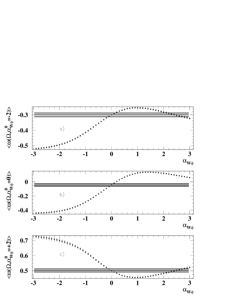
Figure 5: Estimation of the $\alpha_{W\phi}$ coupling based on The average of the Modified Observables for three different expansion pints.

for any value $\vec{\lambda}$ by means of M.C. integration employing the reweighting technique [10]. This procedure is valid for any range of coupling values and consequently guarantees consistent estimation independently of the particular expansion point. The above arguments are demonstrated in figure 4 and 5. A collection of M.C. events, consisted from several sets produced at several couplings and passed through the full detector simulation, had been used to evaluate, by reweighting, the dependence (in the following the calibration curve) of the mean values of the Modified Observables for electronic final states on the $\alpha_{W\phi}$ coupling for several ($\alpha_{W\phi}^{0}=$ -2,0 and 2) expansion points. The points, in these figures, represent the calibration curves whilst the straight lines in figure 4 correspond to the linear equation (49). It is, though, obvious that the consistency of an estimation based on the linear relation (49), as proposed in [9], depends strongly on the expansion point. However, when the calibration curve is used, the estimation is consistent independently of the expansion point, as is shown in figure 5 where a set of a M.C. electronic events have been used as a data sample. These events were generated with the EXCALIBUR four fermion generator with Standard Model couplings and passed through a full detector simulation. The mean values of the Modified Observables evaluated using the data sample as follows:

$$\langle\omega_{k}(\vec{\Omega};\alpha_{W\phi}^{0})\rangle\simeq\frac{1}{N}\sum_{n=1}^{N}\frac{y_{1}(\Omega_{n};\alpha_{W\phi}^{0})}{y_{0}(\Omega_{n};\alpha_{W\phi}^{0})}$$ (55)

are shown in figures 5a), 5b) and 5c) as the central horizontal lines whilst the band around the central line corresponds to the statistical error of (55). Although the calibration curves coincide with the measured averages at the true coupling value independently of the expansion point, the error in the coupling estimation varies, reaching its minimum at the expansion point which equals the true coupling value.

The extended Modified Observable estimators which take into account the expected event multiplicity are built in the same way as in the ideal case, i.e. as the product:

$$\mu(\vec{\lambda})\cdot\int\omega_{k}(\vec{\Omega};\vec{\lambda}^{0})\cdot P(\vec{\Omega};\vec{\lambda})d\vec{\Omega}$$

The calibration functions

$${\cal{F}}_{k}(\vec{\lambda};\vec{\lambda}^{0})=\mu(\vec{\lambda})\cdot\int\omega_{k}(\vec{\Omega};\vec{\lambda}^{0})\cdot P(\vec{\Omega};\vec{\lambda})d\vec{\Omega}$$ (56)

are evaluated as before by reweighted M.C. integration and the coupling estimates are the solutions of the following system of $\rho$ equations with $\rho$ unknowns:

$$\sum_{n=1}^{N}\frac{y_{1}^{k}(\vec{\Omega}_{n};\vec{\lambda}^{0})}{y_{0}(\vec{\Omega}_{n};\vec{\lambda}^{0})}={\cal{F}}_{k}(\hat{\lambda};\vec{\lambda}^{0})$$ (57)

Since the estimation efficiency becomes optimal only when $\hat{\lambda}\simeq\vec{\lambda}^{0}$, the estimation being consistent for each $\vec{\lambda}^{0}$, an iterative procedure can be followed which will converge to the above optimality condition. To demonstrate the convergence properties of this algorithm, three M.C. samples of 1000 $WW\rightarrow e\nu_{e}q\bar{q}$ events each, passed through detector simulation and generated with the EXCALIBUR four fermion generator with $\alpha_{W\phi}$ coupling values equal to -2,0 and +2 respectively, were fitted by solving equation (57) for several values of the expansion point ($\alpha_{W\phi}^{0}$). After every fit, the difference between the estimated value of the coupling and the expansion value $\alpha_{W\phi}^{0}$ defines the step of the iterative procedure. Convergence is achieved at the expansion point where the step equals to zero. As it is shown in figure 6, convergence is achieved after few only (two) iterations almost independently of the initial values.

In the general case, where the data sample consists of a collection of the three semileptonic channels (muonic, electronic and tau), the p.d.f. is the following weighted sum of the individual distributions:

$$P(\vec{\Omega};\vec{\lambda}) = \sum_{f=1}^{3}w_{f}(\lambda)\cdot\int g_{f}(\vec{V};\vec{\lambda})\cdot R_{f}(\vec{V},\vec{\Omega})d\vec{V}$$

$$= \sum_{f=1}^{3}w_{f}(\lambda)\cdot P_{f}(\vec{\Omega};\vec{\lambda})$$

$$P_{f}(\vec{\Omega};\vec{\lambda}) = \int g_{f}(\vec{V};\vec{\lambda})\cdot R_{f}(\vec{V},\vec{\Omega})d\vec{V}$$

$$w_{f}(\lambda) = \frac{\sigma_{obs}^{f}(\vec{\lambda})}{\sum_{f=1}^{3}\sigma_{obs}^{f}(\vec{\lambda})}$$ (58)

where the subscript $f$ stands for the flavor of the final state lepton. Then the extended Modified Observable estimators are also defined as weighted sums of the form:

$$M(\vec{\lambda})\cdot\sum_{f=1}^{3}w_{f}(\vec{\lambda})\cdot\int\omega_{k,f}(\vec{\Omega};\vec{\lambda}^{0})\cdot P_{f}(\vec{\Omega};\vec{\lambda})d\vec{\Omega}=\sum_{f=1}^{3}\mu_{f}(\vec{\lambda})\cdot\int\omega_{k,f}(\vec{\Omega};\cdot P_{f}(\vec{\Omega};\vec{\lambda})d\vec{\Omega}$$ (59)

where $M(\vec{\lambda})$ stands for the expected number of the events in total, whilst $\mu_{f}(\vec{\lambda})$ denotes the expected number of events in the semileptonic channel $f$. In practice one has to evaluate three sets of calibration curves ${\cal{F}}_{k,f}(\vec{\lambda},\vec{\lambda}^{0})$, one for each channel, and to use the $N(=\sum_{f=1}^{3}N_{f})$ selected events to solve the following system of equations:

$$\sum_{{f}=1}^{3}\sum_{n=1}^{N_{f}}\frac{y_{1,f}^{k}(\vec{\Omega}_{n};\vec{\lambda}^{0})}{y_{0,f}(\vec{\Omega}_{n};\vec{\lambda}^{0})}=\sum_{f=1}^{3}{\cal{F}}_{k,f}(\hat{\lambda};\vec{\lambda}^{0})$$ (60)

5 Numerical Results

In the previous section we proposed two strategies which include the detector effects in efficient estimators. In principle their asymptotic efficiency is less than the unbinned eight-dimensional likelihood estimator due to the projections (41) and (51). There is not a simple way to quantify the loss in information due to the fact that an unbinned maximum likelihood in eight dimensions estimator which includes the detector effects is practically impossible to build. Therefore, it makes more sense to discuss in detail the use and properties of these estimators in extracting the TGC’s especially when one deals with small data samples such as the available data samples at 172 $GeV$ centre of mass energy at LEPII. The examples given bellow concern one parameter fits of different sensitivities, where the estimation of the $\alpha_{W\phi}$, $\alpha_{W}$ and $\alpha_{B\phi}$ couplings have been chosen for this purpose.

In all the following demonstrations the integrations performed by M.C. techniques made use of the reweighting procedures to express accurately integrals as functions of the TGC’s. Several M.C. samples, generated either with the PYTHIA [12] (including only the resonant graphs, and ISR) or the EXCALIBUR (including the full set of four fermion graphs and ISR) generators at different coupling values and having passed through the detector simulation program DELSIM, were reweighted to correspond to the full set of four fermion diagrams with Coulomb corrections. These samples have been combined as in [10], in order to increase the statistical accuracy of the reweighted M.C. integrations. In parallel other M.C. set of events, produced with the EXCALIBUR four fermion generator at certain coupling values, played the role of data sets after being passed through DELSIM. The selection criteria, applied to all the M.C. events, were those described in Section 2. The event multiplicity of each of the M.C. data samples was chosen according to Poissonian distributions with mean values corresponding to the expected number of events after reconstruction with integrated luminosity $\sim~{}10~{}pb^{-1}$ (a typical integrated luminosity received by the LEP experiments at $\sqrt{s}~{}=~{}172~{}GeV$). As an example, the data sets which were produced with Standard Model couplings consist of $n_{\mu}+n_{e}+n_{\tau}$ events, where the subscript denotes the lepton flavor in the final state and the $n_{\mu},n_{e},n_{\tau}$ multiplicities varied from set to set following Poissonian distributions with means 15.35, 12.5 and 5.64 respectively.

5.1 Binned Likelihood Fits

The central assumption in this paper is that the resolution and the selection efficiency can not be expressed easily as functions of eight kinematic variables. Consequently the projected p.d.f. in the $\zeta_{1}(\vec{\Omega})$, $\zeta_{2}(\vec{\Omega})$ plane (44) cannot be expressed analytically. Its numerical evaluation is, though, possible using M.C. events. There are several techniques [11] of functional interpolation but this work followed the simplest, namely, the determination of the projected distribution in bins of $\zeta_{1}$ and $\zeta_{2}$. Then the extended likelihood function, when N events are observed, distributed as $n_{k}$ ($k=1,\ldots 3\cdot\beta$) events (including background contribution) in the $k^{th}$ $\{\zeta_{1},\zeta_{2}\}$ bin, is written as:

$$L^{ext}=\prod_{k=1}^{3\cdot\beta}\frac{1.}{2\cdot\pi\cdot\sigma_{k}(\lambda)\sigma_{bk}}\int\int\frac{(x_{k}+y_{k})^{n_{k}}}{n_{k}!}e^{-(x_{k}+y_{k})}e^{-\frac{(x_{k}-\mu_{k}(\lambda))^{2}}{{2\cdot\sigma_{k}}^{2}(\lambda)}}e^{-\frac{(y_{k}-b_{k})^{2}}{{2\cdot\sigma_{bk}}^{2}}}dx_{k}\cdot dy_{k}$$ (61)

Each of the $\beta$ consecutive terms in this product belongs to one of the three semileptonic final states, whilst $\mu_{k}(\lambda)$ ($b_{k}$) and $\sigma_{k}(\lambda)$ ($\sigma_{bk}$) are the expected number of signal (background) events in the $k^{th}$ bin and the gaussian error respectively. The evaluation of $\mu_{k}(\lambda)$ and its error as a function of the couplings is done by reweighted M.C. integration where the detector effects and the contamination of each of the final state channels from each other have been taken into account. A technical detail, worth mentioning, is the fact that the calculation of the coordinates $\zeta_{1,2}$ from the observed vector $\Omega$ is solely based on the Matrix Elements because other factors, such as the phase space and that expressing the initial state radiation, cancel out in (44).

To demonstrate the statistical properties of this technique, 210 M.C. data samples at Standard Model Couplings and without background contribution were fitted. The produced distributions of the estimated $\alpha_{W\phi},\alpha_{W},\alpha_{B\phi}$ in one-TGC model fits, are shown in figures 7a, 8a and 9a. These distributions are found to be in excellent agreement with Gaussians of means ($0.01\pm 0.02$, $0.007\pm 0.04$ and $0.07\pm 0.1$) consistent with the true coupling values and sigmas equal to $0.34\pm 0.02$,$0.6\pm 0.03$,$1.25\pm 0.05$ respectively. Furthermore the pull distributions, shown in 7b, 8b and 9b are found to be normal with sigmas ($0.94\pm 0.05$, $1.02\pm 0.06$ and $0.97\pm 0.05$) consistent with unity, which indicates that the errors of the estimations are correctly evaluated. This is also supported by the very good agreement of the sigma of the distribution of the estimations and the mean of the distribution of the estimated error in each individual fit ($0.34\pm 0.04$, $0.58\pm 0.05$ and $1.28\pm 0.02$). Similar tests performed with 20 sets produced with $\alpha_{W\phi}$ values at -2, and 2 demonstrated the same properties. .

5.2 Modified Observable Fits

An estimation of the couplings based on the extended Modified Observable technique is expected to be at least equally efficient as the binned extended likelihood estimation of the previous section. Furthermore, the Modified Observable fits do not split the events into bins and in principle they suffer from less systematic error due to the M.C. statistics. However, as has been emphasized in the previous sections, the optimal efficiency of this technique is achieved when the uncertainty on the measurement of the mean of the Modified Observables lies within the linear part of the calibration curve around the expansion point.

The calibration curve (${\cal{F}}(\lambda;\lambda^{0})$) and its statistical error(${\cal{E}}(\lambda;\lambda^{0})$) at the $\lambda^{0}$ expansion point are evaluated by reweighted M.C. integration as functions of the fitted coupling. In the general case, taking also into account the statistical errors due to the finite M.C. statistics, the coupling value is extracted by maximizing the following likelihood function:

$$L(\lambda;\lambda_{0})=\frac{1}{\sqrt{2\cdot\pi\cdot(\sigma_{d}^{2}(\lambda_{0})+\sigma_{b}^{2}(\lambda_{0})+{\cal{E}}^{2}(\lambda;\lambda_{0}))}}\cdot e^{A(\lambda;\lambda_{0})}$$ (62)

where

$$A(\lambda;\lambda_{0})={-\frac{([N\cdot\langle\omega(\Omega;\lambda_{0})\rangle_{data}-N_{b}\cdot\langle\omega(\Omega;\lambda_{0})\rangle_{back}]-{\cal{F}}(\lambda;\lambda_{0}))^{2}}{2\cdot(\sigma_{d}^{2}(\lambda_{0})+\sigma_{b}^{2}(\lambda_{0})+{\cal{E}}^{2}(\lambda;\lambda_{0}))}}$$ (63)

and N is the number of selected events with measured vectors $\{\vec{\Omega}_{1},\ldots\vec{\Omega}_{N}\}$, $N_{b}$ is the number of background events expected in the data sample and $\sigma_{d}(\lambda_{0})$ is the measurement error on the quantity $N\cdot\langle\omega(\Omega;\lambda^{0})\rangle_{data}$ which is evaluated from the data as:

$$N\cdot\langle\omega(\Omega;\lambda_{0})\rangle_{data}\simeq\sum_{f=1}^{3}\sum_{n=1}^{N_{f}}\cdot\frac{y_{1,f}(\Omega_{n};\lambda_{0})}{y_{0,f}(\Omega_{n};\lambda_{0})}$$ (64)

The background term and its error, $\sigma_{b}(\lambda_{0})$ are calculated by using a set of M background M.C. events as:

$$N_{b}\cdot\langle\omega(\Omega;\lambda_{0})\rangle_{back}\simeq\frac{N_{b}}{M}\sum_{i=1}^{M}\cdot\frac{y_{1}(\Omega_{i};\lambda_{0})}{y_{0}(\Omega_{i};\lambda_{0})}$$ (65)

As discussed in the previous sections, an iterative procedure has to be followed until the value of the coupling which maximizes (63) coincides with the expansion point.

As in the case of the binned likelihood estimation, the 210 M.C. sets produced with Standard Model couplings and without background contamination were fitted to determine the $\alpha_{W\phi}$, $\alpha_{W}$ and $\alpha_{B\phi}$ couplings. The results are shown in Figures 10, 11 and 12 where Gaussian fits have been performed to the estimation, pull and estimation error distribution. The technique exhibits the desired properties at least for the case of the $\alpha_{W\phi}$ and $\alpha_{W}$ fits, that is the estimation distributions are found consistent with Gaussians with means at $\langle\hat{\alpha}_{W\phi}\rangle=-0.01\pm 0.02$ and $\langle\hat{\alpha}_{W}\rangle=0.05\pm 0.05$ (which indicates the unbiasedness of the estimation) and sigmas $\sigma_{\alpha_{W\phi}}=0.33\pm 0.02$ and $\sigma_{\alpha_{W}}=0.56\pm 0.03$ which are in excellent agreement with the mean of the distribution of the estimated errors in each individual fit, $0.33\pm 0.04$ and $0.58\pm 0.01$ respectively. The correct estimation of the errors in each fit is also demonstrated by the fact that the pull distributions are normal with sigmas consistent with unity ($1.05\pm 0.07$ for the $\alpha_{W\phi}$ and $0.95\pm 0.06$ for the $\alpha_{W}$ fits). The same properties have been found in estimating $\alpha_{W\phi}$ by using the 20 sets of events produced at -2 and +2 coupling values . However, the fits to extract the $\alpha_{B\phi}$ coupling make apparent that there is a limitation to this technique. Although the distribution of the estimations has a Gaussian shape with mean consistent with the true coupling ($0.08\pm 0.10$) and a sigma equal to $1.25\pm 0.06$, the pull distribution deviates from a Gaussian shape due to an excess of values at pull values around zero. Furthermore the distribution of the estimated errors consists of a gaussian peak centered around 1.3 and of a broad shoulder at higher values which indicates that for a fraction of the fits the error was overestimated. This is a direct consequence of a large statistical error in evaluating the experimental quantity (64) compared to the region in which the approximation (22) is valid .

5.3 Comparison of Fitting Techniques

In order to quantify the loss in precision due to the approximations (41) and (51), the 210 M.C. samples of events used to investigate the properties of the fitting techniques proposed in this paper were used also in unbinned extended likelihood fits by using either the true kinematic vectors of the events (in the following perfect extended likelihood fits) or the reconstructed kinematic vectors after the event has been treated in a 6c constrained fit (in the following 6c unbinned extended likelihood fits). The results of these fits as well as the results of the binned likelihood and the extended Modified Observables fits described in the previous sections are summarized in Table 1. Although the available statistical accuracy provided by this M.C. experimentation with only 210 samples is not enough for strong statements, it can be seen that the 6c unbinned extended likelihood fits, suffer from biases in estimating the $\alpha_{w\phi}$ and $\alpha_{w}$ couplings. These biases are eliminated by application of our proposed techniques.

Since the p.d.f (3) carries less information than the p.d.f (2), it is to be expected that the precisions obtained by the binned 2-dimensional likelihood and the extended Modified Observable methods should be somewhat poorer than those from the perfect EML method. The statistics used for the results of Table 1 are insufficient to demonstrate this conclusively; however, it is clear that the loss of information is very moderate.

6 Conclusions

In this paper it has been shown that the reduction of the necessary kinematic variables in the estimation of TGCs is possible without loosing accuracy. This projection makes it possible to include the detector effects in a binned extended likelihood estimation by employing the reweighting [10] M.C. integration technique. Although this projection is useful only in one TGC parameter fits, an extension of the Optimal Observable technique [9] proposed in this work can further reduce the necessary kinematic parameters to as many Modified Observables as the number of the TGC’s which are fitted simultaneously from the data, while continuing to include the detector effects in the estimators. It is also shown that, by using the reweighting technique, an iterative procedure can be defined with optimal convergence properties.

Both the proposed fitting strategies have been demonstrated to be unbiased estimators when small statistical samples, of the same size as the data sets available from the 172 $GeV$ LEPII run, were fitted. It has been also shown that they consistently evaluate the estimation error. However a limitation of the Modified Observable fits became apparent in evaluating the error in the fitted value of the $\alpha_{B\phi}$ coupling. Such an overestimation is expected in fits where the data are not sensitive to the extracted parameter and will disappear as the available data sets increase in size.

A comparison of the proposed techniques with the unbinned extended likelihood in perfect conditions shows that the estimation accuracy achieved in this analysis is very close to the maximum possible.

Appendix A Appendix A

For $\hat{\lambda}=\vec{\lambda}^{true}$ equation (13) becomes identity. Furthermore by using (9) and approximating $g(\vec{V};\vec{\lambda})$ as in (22) the definition of the maximum likelihood estimator relates the mean values of the Optimum observables ($y_{1}^{i}(\vec{V};\vec{\lambda}^{0})/y_{0}(\vec{V};\vec{\lambda}^{0})$ as:

$$\int\{\frac{y_{1}^{i}(\vec{V};\vec{\lambda}^{0})/y_{0}(\vec{V};\vec{\lambda}^{0})-Z^{i}_{1}(\vec{\lambda}^{0})/Z_{0}(\vec{\lambda}^{0})}{1+\sum_{k=1}^{\rho}[y_{1}^{k}(\vec{V};\vec{\lambda}^{0})/y_{0}(\vec{V};\vec{\lambda}^{0})-Z^{k}_{1}(\vec{\lambda}^{0})/Z_{0}(\vec{\lambda}^{0})]\cdot\hat{\Delta}_{k}}\pm\frac{y_{1}^{i}(\vec{V};\vec{\lambda}^{0})}{y_{0}(\vec{V};\vec{\lambda}^{0})}\}\cdot$$

$$\{\frac{y_{0}(\vec{V};\vec{\lambda}^{0})}{Z_{0}(\vec{\lambda}^{0})}\cdot[1+\sum_{k=1}^{\rho}[y_{1}^{k}(\vec{V};\vec{\lambda}^{0})/y_{0}(\vec{V};\vec{\lambda}^{0})-Z^{k}_{1}(\vec{\lambda}^{0})/Z_{0}(\vec{\lambda}^{0})]\cdot\hat{\Delta}_{k}]\}d\vec{V}=0$$ (66)

where $\hat{\Delta}_{k}=\hat{\lambda}_{k}-\lambda^{0}_{k}$ and the term $y_{1}^{i}(\vec{V};\vec{\lambda}^{0})/y_{0}(\vec{V};\vec{\lambda}^{0})$ has been added and subtracted in the integrand. Then, by expressing the ratio of the integrated quantities as:

$$\frac{Z^{i}_{1}(\vec{\lambda}^{0})}{Z_{0}(\vec{\lambda}^{0})}=\int\frac{y_{1}^{i}(\vec{V};\vec{\lambda}^{0})}{y_{0}(\vec{V};\vec{\lambda}^{0})}\cdot\frac{y_{0}(\vec{V};\vec{\lambda}^{0})}{Z_{0}(\vec{\lambda}^{0})}d\vec{V}$$ (67)

and using (27) the identity (66) becomes :

$$\int O_{i}(\vec{V};\vec{\lambda}^{0})\cdot g(\vec{V};\hat{\lambda})d\vec{V}=$$

$$\int O_{i}(\vec{V};\vec{\lambda}^{0})\cdot g(\vec{V};\vec{\lambda}^{0})d\vec{V}+\sum_{k=1}^{\rho}[\int O_{i}(\vec{V};\vec{\lambda}^{0})\cdot O_{k}(\vec{V};\vec{\lambda}^{0})\cdot g(\vec{V};\vec{\lambda}^{0})d\vec{V}$$

$$-(\int O_{i}(\vec{V};\vec{\lambda}^{0})\cdot g(\vec{V};\vec{\lambda}^{0})d\vec{V})\cdot(\int O_{k}(\vec{V};\vec{\lambda}^{0})\cdot g(\vec{V};\vec{\lambda}^{0})d\vec{V})]\cdot\hat{\Delta_{i}}$$ (68)

which is exactly how the coupling estimators based on the mean of optimal observables have been defined in (28). Thus in the neighborhood of $\vec{\lambda}^{0}$ ( where the approximation (22) is valid) the maximum likelihood estimation is identical to the Optimal Observable estimations and obviously the latter inherits all the properties of the former.

If instead of the likelihood function its extension (31) was used then the extended maximum likelihood estimators will be defined for $N$ observed events as:

$$\sum_{n=0}[\frac{e^{-\mu(\vec{\lambda})}\cdot\mu^{N}}{N!}]_{\vec{\lambda}=\vec{\lambda}^{true}}\cdot\{[\frac{\partial}{\partial{\lambda_{i}}}(\frac{e^{-\mu(\vec{\lambda})}\cdot\mu^{N}}{N!})]_{\vec{\lambda}=\hat{\lambda}}$$

$$+\int[\frac{\partial}{\partial{\lambda_{i}}}\sum_{k=1}^{N}\log{g(\vec{V}_{k};\vec{\lambda})}]_{\vec{\lambda}=\hat{\lambda}}\cdot[\prod_{j=1}g(\vec{V}_{k};\vec{\lambda})]_{\vec{\lambda}=\vec{\lambda}^{true}}d\vec{V}_{1}\cdots d\vec{V}_{N}\}=0$$ (69)

The above condition obviously for $\hat{\lambda}=\vec{\lambda}^{true}$ is an identity which can be reduced, after some algebra, to:

$$\mu(\hat{\lambda})\cdot\int[\frac{\partial}{\partial{\lambda_{i}}}\log{g(\vec{V};\vec{\lambda})}]\cdot g(\vec{V};\vec{\lambda})]_{\vec{\lambda}=\hat{\lambda}}d\vec{V}=0$$ (70)

and when the p.d.f is linearly approximated as in (22) the same expression as (68) is achieved having replaced the terms $O_{i}(\vec{V};\vec{\lambda}^{0})$ with the products $\mu(\hat{\lambda})\cdot O_{i}(\vec{V};\vec{\lambda}^{0})$.

	$\alpha_{w\phi}$	$\alpha_{w}$	$\alpha_{B\phi}$
Perfect Extended Likelihood
mean of estimations	0.006 $\pm$ 0.020	0.01 $\pm$ 0.03	0.11 $\pm$ 0.08
estimation accuracy	0.30 $\pm$ 0.02	0.55 $\pm$ 0.03	1.10 $\pm$ 0.05
6c Unbinned Extended Likelihood
mean of estimations	-0.07 $\pm$ 0.02	0.14 $\pm$ 0.04	0.001 $\pm$ 0.080
estimation accuracy	0.35$\pm$ 0.02	0.65 $\pm$ 0.03	1.14 $\pm$ 0.06
pull sigma	1.10 $\pm$ 0.05	1.35 $\pm$ 0.06	1.03 $\pm$ 0.05
Binned 2 dim. Extended Likelihood
mean of estimations	0.01 $\pm$ 0.02	0.007 $\pm$ 0.040	0.07 $\pm$ 0.10
estimation accuracy	0.34 $\pm$ 0.02	0.60 $\pm$ 0.04	1.25$\pm$ 0.08
pull sigma	0.94 $\pm$ 0.05	1.02 $\pm$ 0.06	0.97 $\pm$ 0.05
Extended Modified Observable
mean of estimations	-0.01 $\pm$ 0.02	0.05 $\pm$ 0.05	0.08 $\pm$ 0.1
estimation accuracy	0.33 $\pm$ 0.02	0.56 $\pm$ 0.03	1.25$\pm$ 0.06
pull sigma	1.05 $\pm$ 0.07	0.95 $\pm$ 0.05	$0.90^{*}$ $\pm$ 0.05

Table 1: Comparison of the statistical properties of the techniques proposed in this paper with the unbinned extended likelihood estimations.(*This value represents the root mean squared of the pulls)

Figure 1: The dependence of $z_{1}(x_{1},x_{2})$ on the $c_{1}(\vec{\Omega})/c_{0}(\vec{\Omega})$ in three different regions (a) 0.00-0.12, b) 0.12-0.25 and c) 0.25-1.00) of $c_{2}(\vec{\Omega})/c_{0}(\vec{\Omega})$ when the $\alpha_{W\phi}$ TGC model is consider for electronic final states. The horizontal error-bars correspond to the size of the bin, whilst the solid line denotes the region of equality between the two plotted quantities.

Figure 2: The dependence of $z_{2}(x_{1},x_{2})$ on the $c_{2}(\vec{\Omega})/c_{0}(\vec{\Omega})$ in three different regions (a) -2.00–0.020, b) -0.20-0.25 and c) 0.25-1.00) of $c_{1}(\vec{\Omega})/c_{0}(\vec{\Omega})$ when the $\alpha_{W\phi}$ TGC model is consider for electronic final states. The horizontal error-bars correspond to the size of the bin, whilst the solid line denotes the region of equality between the two plotted quantities.

Figure 3: The approximated Optimum Observable $a_{1}(\phi;\alpha_{W\phi}^{0})$ , corresponding to the $\alpha_{W\phi}$ coupling for electronic final states, as a function of the quantity $y^{1}_{1}(\vec{\Omega};\alpha_{W\phi}^{0})/y_{0}(\vec{\Omega};\alpha_{W\phi}^{0})$ for several values of $\alpha_{W\Phi}^{0}$ = a) +1 b) 0.5 )c -0.5 d) -1. The horizontal error-bars correspond to the size of the bin, whilst the solid line denotes the region of equality between the two plotted quantities.

Figure 4: The mean value of the $\alpha_{W\phi}$ Modified Observables as a function of the $\alpha_{W\phi}$ for three different values of the expansion point ($\alpha_{W\phi}^{0}=-2,0,+2$). The points with the errors correspond to the reweighted M.C. integration technique whilst the straight lines represents the linear equation (51).

Figure 6: Estimation of the $\alpha_{W\phi}$ coupling based on the mean value of the Modified Observable. Three M.C. sets of events produced with different couplings (a) $\alpha_{W\phi}=-2.$,b) $\alpha_{W\phi}=0.$ and c) $\alpha_{W\phi}=+2.$) were fitted for several values of the expansion point (horizontal axis). The vertical axis represents the difference of the expansion point from the estimated value in each fit.

Figure 7: Results ( a) distribution of the estimations b) pull distribution c) distribution of the estimated errors) of Monte Carlo experimentation concerning the estimation of the $\alpha_{W\phi}$ coupling with binned likelihood fits. The solid lines correspond to gaussian fits.

Figure 8: Results ( a) distribution of the estimations b) pull distribution c) distribution of the estimated errors) of Monte Carlo experimentation concerning the estimation of the $\alpha_{W}$ coupling with binned likelihood fits. The solid lines correspond to gaussian fits.

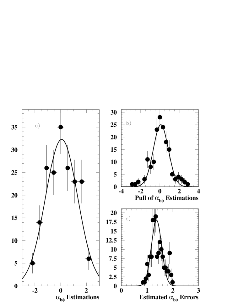
Figure 9: Results ( a) distribution of the estimations b) pull distribution c) distribution of the estimated errors) of Monte Carlo experimentation concerning the estimation of the $\alpha_{B\phi}$ coupling with binned likelihood fits. The solid lines correspond to gaussian fits.

Figure 10: Results ( a) distribution of the estimations b) pull distribution c) distribution of the estimated errors) of Monte Carlo experimentation concerning the estimation of the $\alpha_{W\phi}$ coupling based on the mean value of the Modified Observables. The solid lines correspond to gaussian fits.

Figure 11: Results ( a) distribution of the estimations b) pull distribution c) distribution of the estimated errors) of Monte Carlo experimentation concerning the estimation of the $\alpha_{W}$ coupling based on the mean value of the Modified Observables. The solid lines correspond to gaussian fits.

Figure 12: Results ( a) distribution of the estimations b) pull distribution c) distribution of the estimated errors) of Monte Carlo experimentation concerning the estimation of the $\alpha_{B\phi}$ coupling based on the mean value of the Modified Observables. The solid lines correspond to gaussian fits.

References

- [1] See for example Statistical Methods in Experimental Physics, W.T. Eadie et al, North-Holland P.C. (1988).
- [2] R. L. Sekulin, Phys. Lett. B338 (1994) 369.
- [3] G. Gounaris, J.-L. Kneur and D. Zeppenfeld, in Physics at LEP2, eds G. Altarelli, T. Sjostrand and F. Zwinger, CERN 96-01 Vol. 1,525(1996)
- [4] G Gounaris and C.G. Papadopoulos, DEMO-HEP-96/04, THES-TP 96/11,hep-ph/9612378 (1996)
- [5] C. G. Papadopoulos, Comp. Phys. Comm. 101, (1997) 183.
- [6] F.A. Berends, R. Kleis and R. Pittau, EXCALIBUR, Physics at LEP2, eds G. Altarelli, G. T. Sjostrand and F. Zwinger, CERN 96-01 Vol. 2, 23(1996)
- [7] DELSIM Reference Manual, DELPHI note, DELPHI 87-97 PROG-100
- [8] T.J.V. Bowcock et al., Measurement of Trilinear Gauge Couplings in Collisions at 161 GeV and 172 GeV, DELPHI note 97-113 CONF 95, submitted to the International Europhysics Conference on High Energy Physics, August 1997
-
[9]
M. Diehl and O. Nachtman, Z. Phys. C62 (1994) 397;
C.G. Papadopoulos, Phys. Lett. B386 (1996) 442;
M. Diehl and O. Nachtman, HD-THEP-97-03,CPTH-S494-0197,hep-ph/9702208 (1997) - [10] G.K. Fanourakis, D.A. Fassouliotis and S.E. Tzamarias, A Method to include Detector Effects in Estimators sensitive to the Trilinear Gauge Couplings DEMO-HEP 97/08 (1997).
- [11] See for example Neural Networks for Pattern Recognition by C. M. Bishop, Clarendon Press-Oxford (1995)
- [12] T. Sjöstrand, Comp. Phys. Comm. 82 (1994) 74.