The continuum limit of perturbative coefficients calculated with a large field cutoff

Abstract

We report MC calculations of perturbative coefficients for lattice scalar field theory in dimensions 1, 2 and 3, where the large field contributions are cutoff. This produces converging (instead of asymptotic) perturbative series. We discuss the statistical errors and the lattice effects and show that accurate calculations are possible even in a crossover region where no approximation works. We show that the field cutoff is also a UV regulator. We point out the relevance for QCD questions discussed by Tomboulis and Trottier at this conference.

A central problem in quantum field theory is the presence of different behaviors at different scales. This is clearly the case for QCD [1] where the short distance behavior can be described using perturbation theory, while confinement and other non-perturbative phenomena appear at large distance. A somehow similar situation is encountered in scalar and spin models. We limit here the discussion to the symmetric phase where a trivial high-temperature (strong coupling) fixed point is present. Perturation theory generically fails to provide a proper description of the RG flows near the HT fixed point. From this point of view, the fact that the perturbative series are asymptotic is not surprising.

Asymptotic series can be a serious problem for problems where the strong interactions correction are taken into account. A good example is the hadronic width of the $Z$, where the third order corrections[2] are about two-third of the second order corrections and larger than the experimental error bar for the combined LEP experiments. Perturbative methods also play an important role in the improvement methods[3] that were used to obtain unprecedented accuracy for quantities that can be compared with experiments[4]. Given these recent successes, the standards of accuracy are raised and it is likely that the lack of convergence of QCD series will need to be addressed in the near future.

A simple way[5, 6] to convert an asymptotic series into a convergent one consists in introducing a large field cutoff. It has been shown with three $\phi^{4}$ problems [6] that the modified series converge toward values which are exponentially close to the exact ones. At a fixed order, it is possible to chose the field cutoff in order to optimize the accuracy[7]. The three examples discussed in Ref. [6] can be solved accurately with numerical methods [8, 9]. However, for generic problems, this kind of calculation can be quite difficult, especially in a crossover region (illustrated in Fig. 3) where neither semi-classical methods or HT expansion are available. This difficulty reflects the fact that, in general, the interpolation between RG fixed points is a difficult non-linear problem that has only be solved for simplified models (see [10] for an example).

When no other methods are available, one has to resort to the MC method to perform calculations of the modified perturbative coefficients. In the following, we consider lattice scalar models with nearest neighbor interactions and one component at each site, in 1, 2 or 3 dimensions. For a lattice with $N_{s}$ sites, we will consider the following quantities relevant for perturbation theory:

$$A_{0} = <\sum_{x}\phi^{2}_{x}>/N_{s}$$ (1)

$$A_{1} = <\sum_{x}\phi^{4}_{x}>/N_{s}$$ (2)

$$A_{2} = (<(\sum_{x}\phi^{4}_{x})^{2}>-<\sum_{x}\phi^{2}_{x}>^{2})/N_{s}\ .$$ (3)

The average $<>$ correspond to a Gaussian model where the integration at each site goes from $-\phi_{max}$ to $\phi_{max}$. In $D=1$, the continuum values for $\phi_{max}=\infty$ are $A_{0}=1/2$, $A_{1}=3/4$ and $A_{2}=21/8$. For $D$=2 or 3, $A_{0}$ is UV divergent. Two kinds of errors that should be taken into account: the statistical errors and the errors due to the finite lattice spacing.

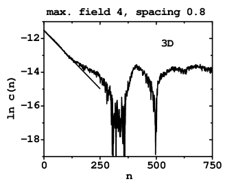
Figure 1: Correlation functions for the observable $A_{0}$ in $D=3$ as a function of the separation $n$ in the configuration number.

The statistical errors decrease as the inverse square root of the number of decorrelated configurations. The correlation times are estimated from the exponential decay of the correlations. If we denote by $O_{i}$ the value of the observable $O$ in a configuration $i$, the correlations $C(n)$ are subtracted averages of $O_{i}O_{i+n}$. Fig. 1 illustrates this exponential decay in an example. Alternatively, we can use Ref. [12] to estimate the statistical error for correlated data.

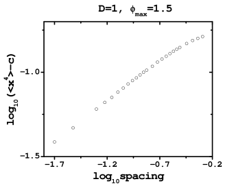
Figure 2: Illustration of the power corrections to $A_{1}$ in $D=1$. We have subtracted the estimated continuum value $c$.

Second, we need to take into account the lattice effects. For small enough lattice spacing $a$, a simple power behavior $c+a^{\alpha}$ is observed, $c$ being the continuum value that we are trying to calculate. The power behavior can be extracted from the statistical fluctuations (which increase when $a$ becomes small!) for an intermediate range of lattice spacing, using a nonlinear fit. This is illustrated in Fig. 2. More detail will be provided in [11].

The comparison between the MC results obtained with the method described above and the accurate numerical results obtained with methods inspired by Ref. [8] is shown below in the case $D=1$ . The MC estimates for $A_{1}$ for various $\phi_{max}$ are compared with accurate values in the table below

$\phi_{max}$ MC Num. 3 0.738(4) 0.7333 2.5 0.646(12) 0.6482 2 0.422(9) 0.4315 1.5 0.178(2) 0.1807 1 0.03987(3) 0.03995

The results for $A_{1}$ and $A_{2}$ are shown in Fig. 3. The MC estimates for $A_{2}$ require a subtraction and are less accurate. We expect that better results can be obtained by improving the statistics and refining the nonlinear fit method.

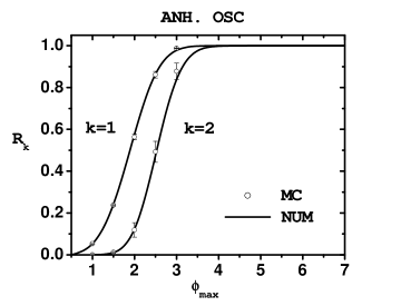
Figure 3: MC (circles) versus accurate numerical results (continuous line) for $A_{1}$ (left) and $A_{2}$ (right). All the values have been divided by their respective infinite cut limits 3/4 and 21/8.

It is possible to calculate approximately the values at the bottom (top) of the curves of Fig. 3 using a HT expansion (semi-classical methods) and reliable interpolation methods are being developed to apprach the crossover region.

$A_{0}$ diverges like Ln($a$) in $D=2$ and $1/a$ in $D=3$, when the lattice spacing $a\rightarrow 0$. However, the field cut takes care of this divergence. This is illustrated in Fig. 4 for $D=2$. This regularization has a simple explanation[13]: since the average (1) provides a positive measure, we can obtain a bound by replacing $\phi_{x}^{2}$ by its maximal value. This yields the bound $A_{0}\leq\phi_{max}^{2}$. The field cut can be thought as produced by an interaction of the form $(\phi/\phi_{max})^{s}$ in the large $s$ limit. Consequently, this should not affect the universal features of the model and it should be possible to calculate the critical exponents using modified perturbative methods. We are planning to extend these methods to gauge theories.

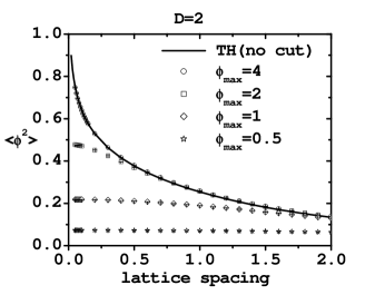
Figure 4: $A_{0}$ for $D$ = 2 as a function of the lattice spacing for various field cuts. The continuous line is the (calculable) lattice result (without cut).

References

- [1] T. Tomboulis, these proceedings, hep-lat/0309006.
- [2] S. A. Larin, T. van Ritbergen, and J. A. M. Vermaseren, Phys. Lett. B320, 159 (1994).
- [3] H. Trottier, these proceedings.
- [4] C. T. H. Davies et al., hep-lat/0304004.
- [5] S. Pernice and G. Oleaga, Phys. Rev. D 57, 1144 (1998).
- [6] Y. Meurice, Phys. Rev. Lett. 88 (2002) 141601.
- [7] B. Kessler, L. Li and Y. Meurice, hep-th/0309022.
- [8] B. Bacus, Y. Meurice, and A. Soemadi, J. Phys. A 28 (1995) L381; Y. Meurice, J. Phys. A 35, 8831 (2002).
- [9] J. J. Godina, Y. Meurice, and M. Oktay, Phys. Rev. D 57 (1998) R6581 and D 59 (1999) 096002.
- [10] Y. Meurice and S. Niermann, J. Stat. Phys. 108, 213 (2002); Y. Meurice, Phys. Rev. E 63, 055101 (Rapid Communication) (2001).
- [11] L. Li and Y. Meurice, U. of Iowa preprint, in preparation.
- [12] C. Daniell, A. Hey, J. Mandula, Phys. Rev. D 30, 2230 (1984).
- [13] We thank H. Sonoda for suggesting the argument.