HU-EP-03/63 DESY 03-138 SFB/CPP-03-34 September 2003
Non–perturbative renormalization of the axial current
with improved Wilson quarks

Abstract

We present a new normalization condition for the axial current, which is derived from the PCAC relation with non–vanishing mass. Using this condition reduces the ${\rm O}(r_{0}m)$ corrections to the axial current normalization constant $Z_{\rm A}$ for an easier chiral extrapolation in the cases, where simulations at zero quark–mass are not possible. The method described here also serves as a preparation for a determination of $Z_{\rm A}$ in the full two–flavor theory.

1 Introduction

Due to the explicit breaking of chiral symmetry in a lattice theory with Wilson quarks a finite renormalization constant $Z_{\rm A}$ for the isovector axial current is needed so that Ward identities take their canonical form up to small lattice corrections. Otherwise a safe extrapolation to the continuum can not be achieved for physical quantities involving this current.

The function $Z_{\rm A}(g_{0})$ [1] currently used by the ALPHA collaboration was obtained by requiring that certain chiral Ward identities are satisfied in the ${\rm O}(a)$ on–shell improved lattice theory up to ${\rm O}(a^{2})$ cutoff effects. This normalization condition is evaluated at zero quark mass and hence the mass term in the PCAC relation was dropped.

However, even in the framework of the Schrödinger functional simulations at vanishing quark mass are not possible if the physical volume, or equivalently the renormalized coupling, is too large. For the large couplings one therefore evaluates the normalization condition at finite quark mass and extrapolates to the chiral point. Since the mass term was ignored in the derivation of the normalization condition this introduces an error of ${\rm O}(r_{0}m)$ in $Z_{\rm A}$. The Sommer scale $r_{0}$ [2] is used as a typical hadronic scale.

Here we present a normalization condition for the axial current, which is derived using the full PCAC relation. This reduces the ${\rm O}(r_{0}m)$ errors in $Z_{\rm A}$ to ${\rm O}(am)$ and therefore results in a much flatter chiral extrapolation.

2 The axial Ward identity

By performing local infinitesimal symmetry transformations of the quark and anti–quark fields in the Euclidean functional integral one derives the Ward identities associated with the chiral symmetry of the continuum action. An axial transformation of the isospin doublet quark fields gives the partially conserved axial current (PCAC) relation

$$\ \langle\partial_{\mu}A_{\mu}^{a}(x){\cal O}\rangle-2m\langle P^{a}(x){\cal O}\rangle=-\langle\delta{\cal O}\rangle,$$ (1)

where $\delta{\cal O}$ is the variation of some operator ${\cal O}$. $A_{\mu}^{a}(x)$ and $P^{a}(x)$ are the isovector axial current and isovector pseudoscalar density, respectively.

Let $\mathcal{R}$ be the space–time region where the chiral transformation is applied. The axial current $A_{\nu}^{b}(y)$ is inserted as an internal operator ($y\!\in\!\mathcal{R}$). If ${\cal O}_{\rm ext}$ denotes a polynomial in the basic fields outside this region the integrated form of the axial current Ward identity is

$$\int_{\partial\mathcal{R}}\!\!\!\textstyle{\rm d}\sigma_{\mu}(x)\,\Big{\langle}A_{\mu}^{a}(x)A_{\nu}^{b}(y){\cal O}_{\rm ext}\Big{\rangle}\qquad\qquad$$

$$\qquad\qquad-2m\int_{R}\!\!{\rm d}^{4}x\,\Big{\langle}P^{a}(x)A_{\nu}^{b}(y){\cal O}_{\rm ext}\Big{\rangle}$$

$$\qquad\qquad\qquad\qquad=i\epsilon^{abd}\Big{\langle}V_{\nu}^{d}(y){\cal O}_{\rm ext}\Big{\rangle}.$$ (2)

The right–hand side of (2) originates from the variation of the internal operator $A_{\nu}^{b}(y)$ since under chiral transformation the axial current rotates into the vector current $V_{\mu}^{a}(x)$.

3 Normalization conditions on the lattice

A normalization condition for the axial current on the lattice is derived by demanding that eq. (2) in terms of the renormalized currents is still valid up to lattice artifacts for a given choice of $\mathcal{R}$ and ${\cal O}_{\rm ext}$.

We use Schrödinger functional boundary conditions in ${\rm O}(a)$-improved lattice QCD [3, 4], i.e. we have an $L^{3}\times T$ space–time cylinder with periodic boundary conditions in the spatial directions and fixed (Dirichlet) boundary condition in the temporal direction.

We choose $\mathcal{R}=L^{3}\times[T/3,2T/3]$ and an ${\cal O}_{\rm ext}$, which creates pseudo-scalar states at the upper and lower temporal boundary. In the renormalization scheme we employ [5, 6] the normalization condition now gives a relation between a set of (improved) correlation functions on the lattice and the renormalization factor $Z_{\rm A}(1+b_{\rm A}am_{q})$.

If the mass is set to zero in (2) with our choice for ${\cal O}_{\rm ext}$ the lattice version of equation (2) becomes

$$\ Z_{\rm A}^{2}f_{AA}^{I}=f_{1},$$ (3)

where $f_{1}$ is the correlator connecting the pseudo-scalar boundary states and $f_{AA}^{I}$ is the correlation function corresponding to the surface integral in (2) in terms of the improved lattice currents.

If the mass term in the PCAC relation (1) is not neglected one has to evaluate an additional correlation function $\tilde{f}_{PA}^{I}$ corresponding to the second term in (2). For this correlator on–shell ${\rm O}(a)$ improvement breaks down due to contact terms. The normalization condition thus obtained is

$$\ Z_{\rm A}^{2}(1\!+\!b_{\rm A}am_{q})^{2}\Big{(}f_{AA}^{I}-2m\tilde{f}_{PA}^{I}\Big{)}=f_{1}.$$ (4)

In the improved theory the normalization conditions (3) and (4) result in an intrinsic uncertainty of ${\rm O}(a^{2})$ in $Z_{\rm A}$. Condition (3) will lead to an additional error of ${\rm O}(r_{0}m)$ when evaluated at finite quark mass whereas (4) will lead to ${\rm O}(am)$ errors from the contact terms in the correlator multiplying the quark mass and also from $b_{\rm A}$, which we only know perturbatively.

4 Testing the new normalization condition

We choose the Schrödinger functional setup with $T=\frac{9}{4}L$, $\theta=0$ and vanishing background field $(C=C^{\prime}=0)$ and evaluate the normalization conditions on $8^{3}\times 18$ quenched lattices with several different values of the hopping parameter.

Figure 1 shows the results from both normalization conditions as a function of the PCAC mass for $\beta=8.0$ on the same set of lattices. In this case a simulation at the chiral point is possible in the Schrödinger functional. As expected the quark mass dependence is strongly reduced when the new normalization condition is used. Also the statistical error in $Z_{\rm A}$ is much smaller with the massive condition.

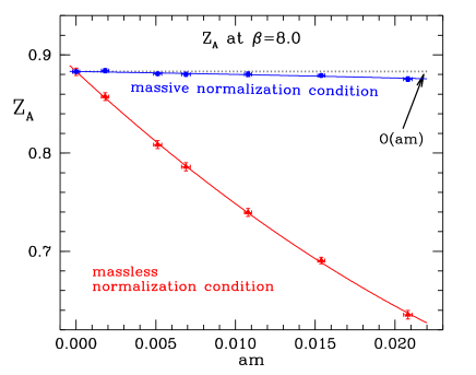
Figure 1: Comparison of old (massless) and new (massive) normalization condition at small coupling. The dotted line is the result for $Z_{\rm A}$.

More interesting is the case of $\beta=6.0$, where $Z_{\rm A}$ has to be extracted from a chiral extrapolation using a quadratic fit. Figure 2 shows that in this case the curvature is more pronounced but the mass dependence for the new method is still quite flat. The error in the extrapolated value for $Z_{\rm A}$ is however larger for the massive normalization condition:

massive $$\,Z_{\rm A}=0.8135(58)$$

massless

(5)

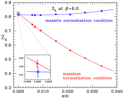
Figure 2: Both normalization conditions evaluated at $\beta=6.0$. The extrapolated values are shown in the insert.

5 Disconnected quark diagrams

On closer inspection the reason for this larger error can be found by looking at the possible Wick contractions for the correlation functions $f_{AA}^{I}$ and $\tilde{f}_{PA}^{I}$. The structure of the external operator used leads to disconnected quark diagrams where the two current insertions each couple to one temporal end of the lattice only.

Those cause large statistical fluctuations especially in the volume correlator $\tilde{f}_{PA}^{I}$, which make the extraction of $Z_{\rm A}$ from the new normalization condition statistically more difficult.

These diagrams can be suppressed by using a different external operator in the derivation of the normalization conditions. This operator requires the existence of a third quark species (spectator) and can therefore be used only as an approximation in a theory with $N_{f}<3$. We are working on an extension of this argument.

Figure 3 shows the result from both conditions if only connected quark diagrams are used. Note that in this case a linear extrapolation in the quark mass is possible. The extrapolated values for $Z_{\rm A}$ in this case are

massive $$\,Z_{\rm A}=0.8135(20)$$

massless .

(6)

Here the new condition not only results in a flat extrapolation, it also gives an extrapolated value of $Z_{\rm A}$, which is consistent with (5) and has a smaller statistical error.

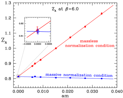
Figure 3: Both normalization conditions using only the connected diagrams.

6 Conclusions

The new normalization condition including the mass term has only a very small dependence on the quark mass. If the spectator quark argument can be extended to the two flavor case it is therefore a suitable tool for calculating the axial current normalization constant in the cases were simulations at zero quark mass are not possible.

This work is also a preparation for an unquenched determination of $Z_{\rm A}$. Due to algorithmic problems at large values of the bare gauge coupling and small quark masses we will benefit greatly from a reliable chiral extrapolation.

We thank M. Lüscher and S. Sint for valuable contributions. This work was supported by the DFG (SFB/TR 09) and the GK271.

References

- [1] M. Lüscher, S. Sint, R. Sommer and H. Wittig, Nucl. Phys. B 491 (1997) 344
- [2] R. Sommer, Nucl. Phys. B 411 (1994) 839
- [3] M. Lüscher, R. Narayanan, P. Weisz and U. Wolff, Nucl. Phys. B 384 (1992) 168.
- [4] S. Sint, Nucl. Phys. B 421 (1994) 135.
- [5] M. Lüscher, S. Sint, R. Sommer and P. Weisz, Nucl. Phys. B 478 (1996) 365.
- [6] K. Jansen et al., Phys. Lett. B 372 (1996) 275