MEM study of true flattening of free energy and the $\theta$ term

Abstract

We study the sign problem in lattice field theory with a $\theta$ term, which reveals as flattening phenomenon of the free energy density $f(\theta)$. We report the result of the MEM analysis, where such mock data are used that ‘true’ flattening of $f(\theta)$ occurs . This is regarded as a simple model for studying whether the MEM could correctly detect non trivial phase structure in $\theta$ space. We discuss how the MEM distinguishes fictitious and true flattening.

1 INTRODUCTION

Lattice field theory with the $\theta$ term suffers from the sign problem. A conventional technique to circumvent it is to perform the Fourier transform of the topological charge distribution $P(Q)$ in order to calculate the partition function ${\cal Z}(\theta)$ [1]. The distribution $P(Q)$ is calculated with real positive Boltzmann weight. However, this still causes flattening of the free energy, which misleads to a fictitious signal of a first order phase transition. To overcome this problem requires exponentially increasing statistics with lattice volume.

We consider the issue of flattening in terms of the maximum entropy method (MEM) [2, 3]. In our previous paper [4] (referred to as (I) hereafter), we used mock data constructed by the Gaussian $P(Q)$ whose corresponding free energy is analytically known to have no singular structure at values of $\theta$ for $0\leq\theta<\pi$ and tested whether the MEM would be effective in the case with flattening as well as without flattening. In the case without flattening, the results of the MEM agree with the exact results. In the case with flattening, the MEM gives smoother $f(\theta)$ than that of the Fourier transform.

In the present work, we consider an opposite case to the above, i.e., consider a model that causes real flattening, which will be explained later. This mimics a case where non trivial phase structure occurs at finite value of $\theta$ $(\theta<\pi)$. We generate mock data based on the model and apply the MEM to them. Our aim is to study (i) whether flattening would be properly reproduced in this model and (ii) how true and fictitious flattening are distinguished in the MEM analysis.

2 MEM AND ‘TRUE’ FLATTENING

The partition function ${\cal Z}(\theta)$ can be obtained by Fourier-transforming the topological charge distribution $P(Q)$:

$${\cal Z}(\theta)=\frac{\int[d\bar{z}dz]e^{-S+i\theta\hat{Q}(\bar{z},z)}}{\int[d\bar{z}dz]e^{-S}}\equiv\sum_{Q}e^{i\theta Q}P(Q),$$ (1)

where $S$ is the action, and $\hat{Q}(\bar{z},z)$ is the topological charge described by lattice fields $z$ and $\bar{z}$. The distribution $P(Q)$ obtained from MC simulations can be decomposed into two parts, a true value and an error of $P(Q)$. When the error at $Q=0$ dominates, the free energy density could develop a flat region in the large $\theta$ region, which misleads one into identifying flattening as a signal of a first order phase transition at a finite value of $\theta$ [5, 6].

Instead of dealing with Eq. (1), we consider

$$P(Q)=\int_{-\pi}^{\pi}d\theta\frac{e^{-i\theta Q}}{2\pi}{\cal Z}(\theta).$$ (2)

The MEM is based on Bayes’ theorem. In our formulation, in order to calculate ${\cal Z}(\theta)$, we maximize the conditional probability, called the posterior probability

$${\rm prob}({\cal Z}(\theta)|P(Q),I,\alpha,m)\propto e^{-\frac{1}{2}\chi^{2}+\alpha S},$$ (3)

where the probability is determined by $\chi^{2}$ and the Shannon-Jaynes entropy $S$ which includes the default model $m(\theta)$

$$S=\int^{\pi}_{-\pi}d\theta\biggl{[}{\cal Z}(\theta)-m(\theta)-{\cal Z}(\theta)\log\frac{{\cal Z}(\theta)}{m(\theta)}\biggr{]}.$$ (4)

Information $I$ plays the important role that enforces ${\cal Z}(\theta)$ to be positive. The parameter $\alpha$ determines the relative weights of $S$. The best image of ${\cal Z}(\theta)$ for a fixed $\alpha$ is then given by

$$\frac{\delta}{\delta{\cal Z}(\theta)}(-\frac{1}{2}\chi^{2}+\alpha S)\Bigm{|}_{{\cal Z}={{\cal Z}^{(\alpha)}}}=0.$$ (5)

This is followed by the successive procedures in order to obtain $\alpha$-independent final image ${\hat{\cal Z}}(\theta)$ [2, 3]: (i) Averaging ${\cal Z}^{(\alpha)}$:

$${\hat{\cal Z}}(\theta)=\int d\alpha~{}{\rm prob}(\alpha|P(Q),I,m){\cal Z}^{(\alpha)}(\theta).$$ (6)

and (ii) error estimation.

In (I), we used the Gaussian $P(Q)$ for the MEM analysis, which is parameterized as

$$P_{\rm G}(Q)\propto\exp[-\frac{c}{V}Q^{2}],$$ (7)

where $c$ is a constant (=7.42) and $V$ is regarded as the lattice volume. In order to address a question whether flattening is due to the statistical error or due to the characteristic of the data themselves, and a question whether these two are distinguished in terms of the MEM, we consider a simple model. Suppose in some lattice theory that calculated $P(Q)$ were slightly deviated from the Gaussian one only at $Q=0$:

$$P(Q)=P_{\rm G}(Q)+p_{0}\times\delta_{Q,0},$$ (8)

where $p_{0}$ is a constant. The partition function is analytically obtained by use of the Poisson sum formula as

$${\cal Z}_{\rm ps}(\theta)\propto\sqrt{\frac{\pi V}{c}}\sum_{n=-\infty}^{\infty}\exp\biggl{[}-\frac{V}{4c}(\theta-2\pi n)^{2}\biggr{]}+p_{0}.$$ (9)

Because the first term in Eq. (9) is monotonically decreasing function of $\theta$ in the region $0\leq\theta\leq\pi$, the second one gives a flat distribution at large values of $\theta$. We generate mock data based on $P(Q)$ in Eq. (8) by adding Gaussian noise with the variance $\delta\times P(Q)$ for each value of $Q$.

3 RESULTS

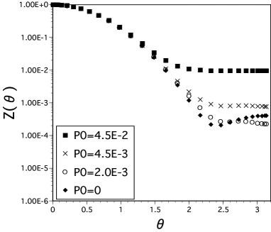
Figure 1: Partition function calculated by numerical Fourier transform for $V=50$. Data for $P(Q)$ are based on Eq. (8) with $p_{0}=4.5\times 10^{-2}$, $4.5\times 10^{-3}$, $2.0\times 10^{-3}$ and $0$.

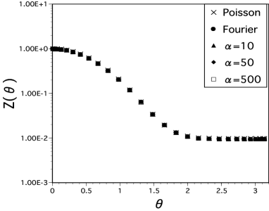
Figure 2: ${\cal Z}^{(\alpha)}(\theta)$ for various values of $\alpha$. Here, $V=50$ and $p_{0}=4.5\times 10^{-2}$.

Figure 1 displays the behavior of ${\cal Z}(\theta)$ calculated by the numerical Fourier transform of Eq. (8) for $V=50$ and various values of $p_{0}$; $p_{0}=4.5\times 10^{-2}$, $4.5\times 10^{-3}$ and $2.0\times 10^{-3}$. The parameter $\delta$ is chosen to be $1/400$. Figure 1 also displays ${\cal Z}(\theta)$ for $V=50$ and $p_{0}=0$, which was studied in (I) in detail. Clear flattening is observed in all the cases. When noise is added, the partition function for Eq. (8) is given by

$${\cal Z}(\theta)=\frac{\sum_{Q}P_{\rm G}(Q)e^{i\theta Q}+p_{0}+\sum_{Q}\Delta P(Q)e^{i\theta Q}}{B},$$ (10)

where $B$ is a normalization constant. When the constant term dominates in the large $\theta$ region, ${\cal Z}(\theta)\approx p_{0}/B$. For $V=50$ and $p_{0}=4.5\times 10^{-2}$, $B$ is numerically estimated as 4.45 and thus ${\cal Z}(\theta)\approx 1.0\times 10^{-2}$. For other choice of $p_{0}$, $4.5\times 10^{-3}$ and $2.0\times 10^{-3}$, $p_{0}/B$ becomes $1.0\times 10^{-3}$ and $4.5\times 10^{-4}$, respectively. These values agree with those of flattening observed in Fig. 1, and we thus find that flattening for these ${\cal Z}(\theta)$ is not caused by the error in $P(Q)$ but is due to the additional term in Eq. (8). On the other hand, flattening for the $p_{0}=0$ case in Fig. 1 is due to the errors in $P(Q)$ as investigated in (I).

Having distinguished two kinds of flattening, we test whether the MEM can properly reproduce the true one. We employ the case for $p_{0}=4.5\times 10^{-2}$, as an example. Figure 2 displays ${\cal Z}^{(\alpha)}(\theta)$ for various values of $\alpha$, which is calculated by Eq. (5). The default model is chosen to be the constant one, $m(\theta)=1.0$. We find that ${\cal Z}^{(\alpha)}(\theta)$ are independent of the values of $\alpha$. They show clear flattening, which are in agreement with the result of the Fourier transform and also with that of the Poisson sum formula, Eq. (9). The probability ${\rm prob}({\cal Z}_{n}|P(Q),I,m)$ shows a narrow peak located at $\alpha\approx 15$. Thus ${\hat{\cal Z}}(\theta)$ agrees with ${\cal Z}^{(\alpha)}(\theta)$ in Fig. 2, and the MEM yields true flattening.

With other choice of the value of $p_{0}$, we repeat the same procedure. For $p_{0}=4.5\times 10^{-3}$, the MEM yields true flattening as in the case $p_{0}=4.5\times 10^{-2}$. This is plotted in Fig. 3. For $p_{0}=1.0\times 10^{-3}$, however, this is not the case. We find that the critical value of $p_{0}$ above which flattening is properly reproduced is $p_{0}\approx 2.0\times 10^{-3}$. This critical value of $p_{0}$ is associated with the magnitude of the error in $P(Q)$.

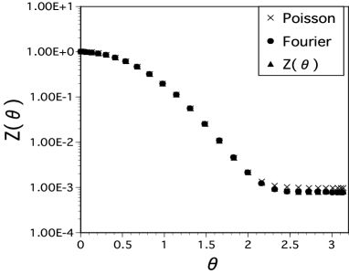
Figure 3: ${\hat{\cal Z}}(\theta)$ for $V=50$ and $p_{0}=4.5\times 10^{-3}$.

In summary, we have applied the MEM to mock data with true flattening and found that flattening is well reproduced. This is in contrast to the case of fictitious flattening studied in (I), where the MEM could predict no fictitious flattening [4]. Applicability of the MEM associated with the magnitude of the errors in $P(Q)$ will be reported elsewhere.

References

- [1] U. -J. Wiese, Nucl. Phys. B318 (1989), 153.
- [2] R. K. Bryan, Eur. Biophys. J. 18 (1990), 165.
- [3] M. Asakawa, T. Hatsuda and Y. Nakahara, Prog. Part. Nucl. Phys. 46 (2001), 459.
- [4] M. Imachi, Y. Shinno and H. Yoneyama, Prog. Theor. Phys. 111 (2004), 387.
- [5] J. C. Plefka and S. Samuel, Phys. Rev. D56 (1997), 44.
- [6] M. Imachi, S. Kanou and H. Yoneyama, Prog. Theor. Phys. 102 (1999), 653.
- [7] R. Burkhalter, M. Imachi, Y. Shinno and H. Yoneyama, Prog. Theor. Phys. 106 (2001), 613.