Non-perturbative scale evolution of four-fermion operators in two-flavour QCD

Abstract:

We apply finite-size recursion techniques based on the Schrödinger functional formalism to determine the renormalization group running of four-fermion operators which appear in the $\Delta S=2$ effective weak Hamiltonian of the Standard Model. Our calculations are done using ${\cal O}(a)$ improved Wilson fermions with $N_{\rm f}=2$ dynamical flavours. Preliminary results are presented for the four-fermion operator which determines the $B_{K}$-parameter in tmQCD.

1 Introduction

A precise determination of the Kaon $B$-parameter is required to constrain the CKM unitarity triangle analysis. $B_{K}$ is defined in terms of hadronic matrix elements which can be computed using lattice QCD. At present, the inclusion of dynamical quark effects is an essential requirement in these lattice calculations. Indeed, a remarkably good agreement has been found between several independent quenched determinations of $B_{K}$ [1], leaving the “quenching” effects as the largest uncertainty. A complete study of the systematic effects, other than quenching, has been performed in ref. [2] and reviewed in this conference [3]. There are indications that once dynamical quarks are taken into account, a major source of uncertainty on lattice results arises from the determination of the renormalization factors of the four-fermion operators [1]. In principle, this uncertainty can be completely eliminated by a non-perturbative renormalization procedure. Similarly, the renormalization group (RG) running of the operator from hadronic scales up to high-energies, where perturbation theory can be safely applied, is best performed non-perturbatively. Here we report on the status of such a non-perturbative renormalization using $N_{\rm f}=2$ dynamical flavours. In particular, we present preliminary results for the scale evolution of the four-fermion operator relevant for the determination of $B_{K}$ in the context of tmQCD [4].

The theoretical description of the $K^{0}-\bar{K}^{0}$ oscillation is controlled, once high-energy scales are integrated through an operator product expansion procedure, by the matrix element $\langle\bar{K}^{0}|O^{\Delta S=2}|K^{0}\rangle$, where the four-fermion operator is defined as follows:

$$O^{\Delta S=2} \equiv [\bar{s}\gamma_{\mu}(1-\gamma_{5})d]\,\,[\bar{s}\gamma_{\mu}(1-\gamma_{5})d]\,\,=\,\,O_{\rm\scriptscriptstyle VV+AA}-O_{\rm\scriptscriptstyle VA+AV}\,.$$ (1)

The strange and down quark fields are denoted by $s$ and $d$ respectively. The $B_{K}$-parameter is expressed in terms of the parity-even $O_{\rm\scriptscriptstyle VV+AA}$ operator :

$$B_{K}\equiv\frac{\langle\bar{K}^{0}|O_{\rm\scriptscriptstyle VV+AA}|K^{0}\rangle}{\frac{8}{3}F_{K}^{2}m_{K}^{2}}\,.$$ (2)

Parity conservation ensures that the matrix element $\langle\bar{K}^{0}|O_{\rm\scriptscriptstyle VA+AV}|K^{0}\rangle$, involving the parity-odd operator, is identically zero.

In lattice regularizations preserving chiral symmetry the operator $O_{\rm\scriptscriptstyle VV+AA}$ is multiplicatively renormalizable. This is not the case for Wilson fermions because in this case chiral symmetry is broken at non-zero lattice spacing. The renormalization of $O_{\rm\scriptscriptstyle VV+AA}$ is therefore more involved since mixing with four other dimension-6 operators has to be considered. On the other hand, discrete symmetries protect the parity-odd operator $O_{\rm\scriptscriptstyle VA+AV}$, so as to preserve multiplicative renormalization also in the case of Wilson fermions [5, 6].

The inclusion of a “twisted mass” term in the fermionic action opens the way to improve the renormalization properties of Wilson fermions. The twisted-mass theory is related to standard QCD through an axial transformation of the quarks fields. By choosing appropriate formulations of tmQCD (see ref. [2] for two of these formulations), it is possible to relate the QCD $O_{\rm\scriptscriptstyle VV+AA}$ operator to a partner $O_{\rm\scriptscriptstyle VA+AV}$ in tmQCD where the property of multiplicative renormalization of this operator is preserved. This method allows the determination of $B_{K}$ only via multiplicative renormalization, thus avoiding mixing with operators of wrong chirality. Another proposal in this direction uses chiral Ward-Takahashi identities to relate parity-odd and parity-even operators [7].

Our strategy to renormalize the operator $O_{\rm\scriptscriptstyle VA+AV}$ closely follows the one used in ref. [8] for the quenched case. The connection between the renormalization group invariant operator $\hat{O}_{\rm\scriptscriptstyle VA+AV}$ and its bare counterpart $O_{\rm\scriptscriptstyle VA+AV}(g_{0})$ can be written in the following way:

$$\hat{O}_{\rm\scriptscriptstyle VA+AV}(x)=\lim_{g_{0}\rightarrow 0}\,\,\,\mathcal{Z}_{\rm\scriptscriptstyle VA+AV;s}(g_{0})\,\,\,O_{\rm\scriptscriptstyle VA+AV}(x;g_{0})\,.$$ (3)

The RGI operator is independent of the renormalization scheme and scale when the renormalization conditions are imposed at zero quark mass [9]. The renormalization factor $\mathcal{Z}_{\rm\scriptscriptstyle VA+AV;s}(g_{0})$ is scale-independent but depends on the scheme $s$ (only through cutoff effects) and on the lattice regularization. These dependences are manifest when decomposing $\mathcal{Z}_{\rm\scriptscriptstyle VA+AV;s}(g_{0})$ into:

$$\mathcal{Z}_{\rm\scriptscriptstyle VA+AV;s}(g_{0})=\hat{Z}_{\rm\scriptscriptstyle VA+AV;s}(\mu_{\rm min})\,Z_{\rm\scriptscriptstyle VA+AV;s}(g_{0},a\mu_{\rm min})\ .$$ (4)

The first factor on the r.h.s. of eq. (4) controls the RG-running of the operator from the reference scale $\mu_{\rm min}$ to an infinite scale. It is independent of the regularisation. The second factor, $Z_{\rm\scriptscriptstyle VA+AV;s}(g_{0},a\mu_{\rm min})$, relates the bare lattice operator to its continuum value at the hadronic scale $\mu_{\rm min}$. This factor is therefore dependent on both the regularization and the scale. Both factors on the r.h.s. of eq. (4) depend on the renormalization scheme. In this report, we focus on the more expensive part of the renormalization procedure, that is, the computation of the contribution of the non-perturbative evolution function $\hat{Z}_{\rm\scriptscriptstyle VA+AV;s}(\mu_{\rm min})$ describing the running in the scale range $1$ GeV – $100$ GeV.

2 Renormalization group running of four-fermion operators

Let us first define a renormalized four-fermion operator $O_{R}$ at a reference scale $\mu$ :

$$O_{R}(x;\mu)=\lim_{a\rightarrow 0}\,\,\,Z_{O}(g_{0},a\mu)\,\,\,O(x;g_{0})\,.$$ (5)

The running of the renormalized operator $O_{R}(\mu)$ is controlled by its anomalous dimension $\gamma_{O}(\bar{g})$, defined as :

$$\mu\,\,\,\frac{\partial}{\partial\mu}O_{R}(x;\mu)=\gamma_{O}(\bar{g})\,\,\,O_{R}(x;\mu)\ .$$ (6)

In mass-independent renormalization schemes [9] as those we consider here, the function $\gamma_{O}(\bar{g})$ only depends on the renormalized coupling $\bar{g}$. The perturbative expansion of $\gamma_{O}(\bar{g})$ is given by

$$\gamma_{O}(g)\stackrel{{\scriptstyle g\to 0}}{{\sim}}-g^{2}\left(\gamma_{O}^{(0)}+\gamma_{O}^{(1)}g^{2}+\gamma_{O}^{(2)}g^{4}+\ldots\right)\ ,$$ (7)

with $\gamma_{O}^{(0)}$ a universal coefficient. By combining eqs. (5) and (6), it is possible to relate the anomalous dimension of $O_{R}$ to its scale-dependent renormalization factor :

$$\gamma_{O}(\kern 1.0pt\overline{\kern-1.0ptg\kern 0.0pt}\kern 1.0pt(\mu))=\lim_{a\to 0}\left(\mu\frac{\partial}{\partial\mu}Z_{O}(g_{0},a\mu)\right)Z_{O}(g_{0},a\mu)^{-1}\ .$$ (8)

The RGI operator is obtained upon the formal integration of eq. (6). It is given by

$$\hat{O}(x)\,\,=\,\,O_{R}(x;\mu)\,\,\,\left[\frac{\bar{g}^{2}(\mu)}{4\pi}\right]^{-\gamma_{O}^{(0)}/(2b_{0})}\exp\left\{-\int_{0}^{\bar{g}(\mu)}dg\left(\frac{\gamma_{O}(g)}{\beta(g)}-\frac{\gamma_{O}^{(0)}}{b_{0}g}\right)\right\}\,.$$ (9)

The integral in the r.h.s of eq. (9) describes the scale evolution of $\gamma_{O}(\bar{g})$. The evolution function of the operator $O_{R}$ between the renormalization scale $\mu$ and an arbitrary scale $\mu^{\prime}$ is given by:

$$U(\mu^{\prime},\mu)\equiv\exp\left\{\int_{\kern 1.0pt\overline{\kern-1.0ptg\kern 0.0pt}\kern 1.0pt(\mu)}^{\kern 1.0pt\overline{\kern-1.0ptg\kern 0.0pt}\kern 1.0pt(\mu^{\prime})}\frac{\gamma_{O}(g)}{\beta(g)}{\rm d}g\right\}=\lim_{a\to 0}\frac{Z_{O}(g_{0},a\mu^{\prime})}{Z_{O}(g_{0},a\mu)}\ .$$ (10)

The running of the renormalized four-fermion operator $O_{R}$ can therefore be performed by constructing ratios of the renormalization factors $Z_{O}$ at different scales.

Our renormalization schemes are defined in the Schrödinger functional (SF) formalism. This technique has been used to determine the scale evolution of physical quantities such as the strong coupling [10, 11] or the quark mass [12, 13]. These studies were performed both with and without dynamical quarks. In the case of four-fermion operators [8] the running was carried out in the quenched approximation. We regularize the theory on a lattice of physical size $L^{4}$ using standard SF boundary conditions allowing to carry out simulations at zero quark masses. The SF is used as a mass-independent renormalization scheme; since the renormalization factors are flavour-independent, they can also be used to renormalize the $B$-parameters in the Kaon, $D$ and $B$-meson sectors. The renormalization conditions are imposed at a scale $\mu$ equal to the IR cutoff $1/L$.

Let us now concentrate on the case of the local parity-odd four-fermion operator:

$$O_{\rm\scriptscriptstyle VA+AV}(x)=\frac{1}{2}\left[(\bar{\psi}_{1}\gamma_{\mu}\psi_{2})(\bar{\psi}_{3}\gamma_{\mu}\gamma_{5}\psi_{4})+(\bar{\psi}_{1}\gamma_{\mu}\gamma_{5}\psi_{2})(\bar{\psi}_{3}\gamma_{\mu}\psi_{4})+(\psi_{2}\leftrightarrow\psi_{4})\right]\,.$$ (11)

Four distinct valence flavours are used in the definition of the operator. The SF correlation functions used to extract the operator $O_{\rm\scriptscriptstyle VA+AV}(x)$ are:

$${\cal F}_{[\Gamma_{\rm A},\Gamma_{\rm B},\Gamma_{\rm C}]}(x_{0})=\frac{1}{L^{3}}\langle{\cal O}_{21}[\Gamma_{\rm A}]{\cal O}_{45}[\Gamma_{\rm B}]\,\,\,O_{\rm\scriptscriptstyle VA+AV}(x)\,\,\,{\cal O}^{\prime}_{53}[\Gamma_{\rm C}]\rangle\,,$$ (12)

where ${\cal O}$ and ${\cal O}^{\prime}$ are the interpolating fields on the time boundaries (refer to [8] for a full explanation of the notations). Several choices of the Dirac matrices $\Gamma_{\rm A,B,C}$ are allowed. We will focus here on the particular choice $\Gamma_{\rm A}=\Gamma_{\rm B}=\Gamma_{\rm C}=\gamma_{5}$. Note that a “spectator” valence quark $\psi_{5}$ is used in eq. (12). It is useful to keep in mind that since the quarks are massless in this mass-independent renormalization scheme, flavour only enters through Wick contractions.

The logarithmic divergences of the local operator $O_{\rm\scriptscriptstyle VA+AV}(x)$ are isolated by dividing out from the correlator ${\cal F}$ the divergences coming from the boundaries and the external legs. This is obtained through the ratio:

$$h(x_{0})=\frac{{\cal F}_{[\gamma_{5},\gamma_{5},\gamma_{5}]}(x_{0})}{f_{1}^{3/2}},$$ (13)

where $f_{1}$ is the boundary-to-boundary correlation function :  $f_{1}=-1/(2L^{6})\,\langle{\cal O}^{\prime}_{12}[\gamma_{5}]\,\,\,{\cal O}_{21}[\gamma_{5}]\rangle\,.$ The renormalized ratio $h_{R}$ can be written as follows:

$$h_{\rm R}(x_{0};\mu)=Z_{\rm\scriptscriptstyle VA+AV}(g_{0},a\mu)\,h(x_{0};g_{0})\ ,$$ (14)

where the renormalization factor is fixed by imposing the renormalization condition :

$$Z_{\rm\scriptscriptstyle VA+AV}(g_{0},a\mu=1/L)h(x_{0}=L/2;g_{0})=h_{\rm s}(x_{0}=L/2;g_{0})\bigg{|}_{g_{0}=0}\,\,,$$ (15)

i.e. at tree level $Z_{\rm\scriptscriptstyle VA+AV}=1$. The renormalization condition is taken at the scale $\mu=1/L$ and therefore at fixed renormalized coupling $u=\kern 1.0pt\overline{\kern-1.0ptg\kern 0.0pt}\kern 1.0pt^{2}(1/L)$. Note that as the quarks are massless, once the continuum limit $a\to 0$ is taken, the only remaining scale is $L$.

The running of the scale-dependent factor $Z_{\rm\scriptscriptstyle VA+AV}(g_{0},a\mu)$ is implemented in the SF formalism via the step scaling function (SSF), defined in the continuum as:

$$\sigma_{\rm\scriptscriptstyle VA+AV}(u)=\lim_{a\to 0}\Sigma_{\rm\scriptscriptstyle VA+AV}(u,a/L)\,,\hskip 28.45274pt\Sigma_{\rm\scriptscriptstyle VA+AV}(u,a/L)=\frac{Z_{\rm\scriptscriptstyle VA+AV}(g_{0},a/2L)}{Z_{\rm\scriptscriptstyle VA+AV}(g_{0},a/L)}\Bigg{|}_{m=0,~{}\kern 1.0pt\overline{\kern-1.0ptg\kern 0.0pt}\kern 1.0pt^{2}(1/L)=u}\,\,.$$ (16)

The SSF can be written in terms of the evolution function $U$:  $\sigma_{\rm\scriptscriptstyle VA+AV}(u)=U_{\rm\scriptscriptstyle VA+AV}({1}/{2L},{1}/{L})\,.$ The SSF is used to run the operator $O_{\rm\scriptscriptstyle VA+AV}$ between two scales differing by a factor of two. By iterating this procedure the running of the operator can be performed over a large range of scales.

3 Non-perturbative study of the step scaling function

The computation of the SSF is performed with $N_{\rm f}=2$ flavours of ${\cal O}(a)$ improved Wilson fermions. We evaluate $\Sigma_{\rm\scriptscriptstyle VA+AV}(u,a/L)$ at six values of the renormalized coupling $u$ (labelled, in increasing order, $u1,...,u6$). At each of these couplings, we consider three lattice resolutions $L/a=6,8,12$ to extrapolate our data to the continuum limit. The unquenched configurations employed in our computation have been previously used in the study of the quark mass renormalization [13] (the description of our simulation setup can be found in this reference). In fig.1 we present the status of the ongoing determination of $\Sigma_{\rm\scriptscriptstyle VA+AV}(u,a/L)$. Data for some of the simulation points has not yet been included as it is still being generated. Moreover, the statistical errors of our preliminary data in fig.1 will reduce when the complete set of configurations will be considered. The integrated autocorrelation times are included in the error estimate. We observe that the autocorrelations grow when increasing the coupling and when approaching the continuum limit.

The ${\cal O}(a)$ improvement of the dimension-six operator $O_{\rm\scriptscriptstyle VA+AV}$ has not been implemented. Although a Symanzik improvement program is possible, the mixing of $O_{\rm\scriptscriptstyle VA+AV}$ with several dimension-seven operators makes it unpractical. For each of the couplings $u$, the continuum limit of $\Sigma_{\rm\scriptscriptstyle VA+AV}(u,a/L)$ should therefore be taken through a linear extrapolation. This is illustrated in fig.1 in those cases where three $L/a$ resolutions are already available. As our data seems to show rather small cutoff effects, we have also tried to fit $\Sigma_{\rm\scriptscriptstyle VA+AV}(u,a/L)$ to a constant (we perform a weighted average and, somehow abusively, we refer to it as a “constant fit”). In the case of the couplings $u1,u3,u5$ and $u6$ this fit was performed by discarding the $L/a=6$ data which, being far from the continuum, is expected to contain large cutoff effects. By comparing the linear and the constant fit, we observe good agreement of the extrapolated values. A more refined analysis of the continuum extrapolation will be undertaken once our complete set of data will be available.

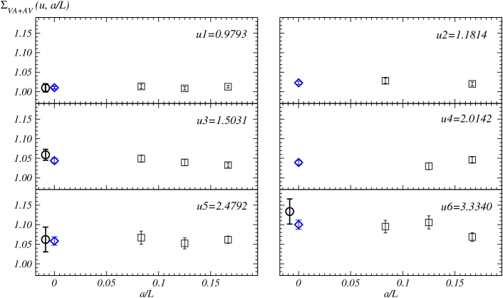
Figure 1: Continuum extrapolation of the SSF $\Sigma_{\rm\scriptscriptstyle VA+AV}(u,a/L)$ at fixed renormalized couplings $u$. The empty circles correspond to the extrapolated value obtained through a linear fit and the diamond to the one obtained via a fit to a constant. Results are preliminary.

In a tentative study of the quality of our data, we present in fig. 2 the SSF $\sigma_{\rm\scriptscriptstyle VA+AV}(u)$. The $N_{\rm f}=2$ data is compared to the quenched one from ref. [8]. The same renormalization scheme and fitting procedures is used in both the $N_{\rm f}=2$ and $N_{\rm f}=0$ data (in particular, also in the quenched case we perform a constant fit to the continuum).  In the strong coupling regime, $u\sim 3.5$, we observe a similar pattern in the $N_{\rm f}=2$ and $N_{\rm f}=0$ data when comparing the value of $\sigma_{\rm\scriptscriptstyle VA+AV}(u)$ obtained through a linear and a constant extrapolation to the continuum: in both $N_{\rm f}=0,2$ cases the linear extrapolation points lie above the constant-fit ones. Due to large statistical errors, the $N_{\rm f}=2$ data shows a better agreement between linear and constant fit. In fig.2, we also plot the perturbative expressions of $\sigma_{\rm\scriptscriptstyle VA+AV}(u)$ in both the $N_{\rm f}=2$ and $N_{\rm f}=0$ cases. These expressions were computed at next-to-leading order (NLO) in ref. [14]. In our chosen renormalization scheme, we observe a fairly good agreement between the perturbative curve and the non-perturbative data in the small coupling region and some signs of deviations in the strong coupling regime. We have considered nine different renormalization schemes (for the definitions of these schemes, refer to [8, 14]). The empirical criterion to identify the more appropriate schemes is to consider those having a small NLO term, of the same sign as the LO one, in the perturbative expansion of $\sigma_{\rm\scriptscriptstyle VA+AV}(u)$. We have checked that our best available scheme is indeed the one of  eq. (13).

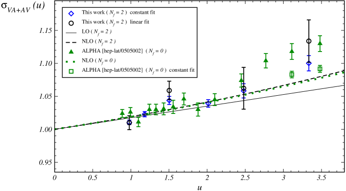
Figure 2: The step scaling function $\sigma_{\rm\scriptscriptstyle VA+AV}(u)$ (discrete points) is compared to the LO and NLO perturbative results. In order to evaluate the quality of our data we compare our $N_{\rm f}=2$ results with quenched data from ref. [8]. Results are preliminary.

Conclusions

We have presented the status of the computation of the non-perturbative RG running of the four-fermion operator $O_{\rm\scriptscriptstyle VA+AV}$ using lattice QCD with two dynamical quarks. This calculation will soon allow us to determine the universal renormalization factor $\hat{Z}_{\rm\scriptscriptstyle VA+AV;s}(\mu)$ in eq. (4). The second factor on the r.h.s of this equation is simpler to determine, compared to $\hat{Z}_{\rm\scriptscriptstyle VA+AV;s}(\mu)$, as it depends only on a single scale $\mu$. This determination will allow to complete the renormalization of the operator $O_{\rm\scriptscriptstyle VA+AV}$. As our renormalization scheme is flavour-independent, the same renormalization factors can be used to determine the $B$-parameters in the strange, charm and beauty sectors.

References

- [1] C. Dawson, PoS LAT2005 (2006) 007.
- [2] P. Dimopoulos et al., [ALPHA Collaboration], Nucl. Phys. B 749 (2006) 69 [hep-ph/0601002].
- [3] C. Pena, “Twisted mass QCD for weak matrix elements,” PoS LAT2006 (2006) 019.
- [4] R. Frezzotti et al., JHEP 0108 (2001) 058 [hep-lat/0101001].
- [5] C. W. Bernard, T. Draper, G. Hockney and A. Soni, Nucl. Phys. Proc. Suppl. 4 (1988) 483.
- [6] A. Donini et al., Eur. Phys. J. C 10 (1999) 121 [hep-lat/9902030].
- [7] D. Becirevic et al., Phys. Lett. B 487 (2000) 74 [hep-lat/0005013].
- [8] M. Guagnelli et al., [ALPHA Collaboration], JHEP 0603 (2006) 088 [hep-lat/0505002].
- [9] S. Weinberg, Phys. Rev. D8 (1973) 3497.
- [10] M. Lüscher, R. Sommer, P. Weisz and U. Wolff, Nucl. Phys. B 413 (1994) 481 [hep-lat/9309005].
- [11] M. Della Morte et al., [ALPHA Collaboration], Nucl. Phys. B 713 (2005) 378 [hep-lat/0411025].
- [12] S. Capitani et al., [ALPHA Collaboration], Nucl. Phys. B 544 (1999) 669 [hep-lat/9810063].
- [13] M. Della Morte et al., [ALPHA Collaboration], Nucl. Phys. B 729 (2005) 117 [hep-lat/0507035].
- [14] F. Palombi, C. Pena and S. Sint, JHEP 0603 (2006) 089 [hep-lat/0505003].