Quark anti-quark expectation value in finite volume

Abstract

We have computed the quark anti-quark expectation value in finite volume at two loop in chiral perturbation theory and compare it with a formula obtained in analogy to the Lüscher formula for pion mass in finite volume. We observe that due to the small finite size correction at two loop it is not possible to obtain conclusions on the accuracy of the extended Lüscher formula.

I Introduction

Quantum chromo dynamics (QCD) is a strongly coupled theory at low energy. Therefore it is difficult to study the physics below the QCD scale of about 1 GeV. Lattice QCD on the other hand is an attempt to tackle this problem by taking the Lagrangian and calculating (parts of) the generating functional numerically. Although these computations with fairly small quark masses are now possible, at the same time the finite volume effects are also becoming important. In this work we employ chiral perturbation theory (ChPT) in order to study these effects analytically. Chiral perturbation theory, in its modern form, was first proposed by Weinberg Weinberg and extended in GL1 ; BCE . ChPT is an effective field theory to describe the strong interactions at low energy. To do the computation in finite volume as suggested in GL2 one imposes a periodic boundary condition on fields which result in the momentum quantization and consequently modification on the quantum corrections. Since the applicability of ChPT is limited to small momenta, in finite volume this leads to

$$F_{\pi}L>1\,.$$ (1)

which holds for L larger than about 2 fm. $F_{\pi}$ is the pion decay constant and L is the linear size of the boundary. In addition we stay in a limit where the Compton wavelength of the pion is smaller than the lattice size which corresponds to

$$m_{\pi}^{2}F_{\pi}^{2}V>>1\,.$$ (2)

This is the so-called p-regime. This condition ensures that perturbative treatment will work. Expectation value of the quark condensate per se will be achieved by varying the generating functional with respect to the scalar external field as follows

$$<\overline{q}T^{a}q>=\frac{1}{Z_{0}}(-i\frac{\delta}{\delta S_{a}})Z_{eff}[s_{a}]_{\arrowvert s_{a}=0}.$$ (3)

Where $T^{a}$ stands for the Gell-Mann matrices. We then carry out the $\langle\overline{q}q\rangle$ at two loop in finite volume within the framework of chiral perturbation theory. This quantity has already been evaluated at one loop order in DG . Another way for the computation of the finite volume effect is the Lüscher approach. In this method one obtains the leading finite size effects for the pion mass to all order in perturbation theory from the scattering amplitude Luscher1 ; Luscher2 . It has later been extended to evaluate the volume dependence of the pion decay constantCH1 . As the second goal we shall then obtain a formula for the the quark condensate volume dependence by following the same line of reasoning as in the Lüscher work. This work was published in Ref. BGH .

II A Lüscher formula for the vacuum condensate

We were inspired by the work of Lüscher, where he showed how the finite size effect on the masses of spin-less particles are related to the forward elastic scattering amplitude in infinite volume. This occurs when particles are enclosed in a lattice box and as considered in this letter with temporal direction of the space-time extended to infinity. To see explicitly where these effects stem from, one looks at the two-point correlation function with fields subjected to a periodic boundary condition. The correlator takes on the form

$$<\phi(x)\phi(0>_{L}=\int\frac{dp_{0}}{2\pi}\sum_{\vec{p}}L^{-d}e^{-ip.x}G_{L}^{-1}(\vec{p}^{2},m_{0}^{2})$$ (4)

where the inverse propagator reads

$$G_{L}(\vec{p}^{2},m_{0}^{2})=p^{2}-m_{0}-\Sigma_{L}(p^{2})$$ (5)

and $\Sigma_{L}(p^{2})$ denotes the sum of the one-particle irreducible diagrams to be evaluated in momentum space with discretized momenta and $\vec{p}=\frac{2\pi\vec{n}}{L}$, with $\vec{n}$ a three dimensional vector of integers. In practice the desired quantity to compute is the change in $\Sigma(p^{2})$ due to the finite volume correction and the difficult task in Lüscher’s work was to show that this consists of all self-energy diagrams with just one propagator in each diagram allowed to wrap around the whole position space and therefore experiencing the boundary. Using the Poisson summation formula the modified propagator can be obtained in terms of the propagator in the infinite volume accompanied by an exponential factor as follows

$$G_{L}(q)=\sum_{\vec{n}}e^{-iq_{i}n_{i}L_{i}}G_{\infty}$$ (6)

where in three dimensions the length squared for a given $\vec{n}$ reads $k=\vec{n}^{2}=n_{1}^{2}+n_{2}^{2}+n_{2}^{2}$. For $\vec{n}=0$ it gives back the propagator in infinite volume. The crucial point comes about in Euclidean space where $q_{0}\to-iq_{0}$ and, as shown below, in our result for $\langle\bar{q}q\rangle$ the exponential factor falls off rapidly for large $\vec{n}^{2}$. Lüscher in his analysis kept only $\vec{n}^{2}=1$ but summation over all values shall be carried out numerically in our formula as suggested in CH2 .

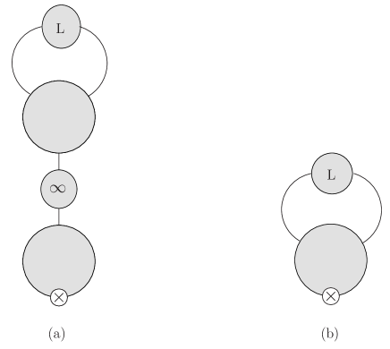
Figure 1: Two potentially relevant graphs to the $\langle\bar{q}q\rangle$.
$\otimes$ indicates the insertion of $\langle\bar{q}q\rangle$ and the solid line is the meson propagator BGH .

Out of three self-energy graphs shown in Ref. Luscher1 , only two are potentially relevant to the $\langle\bar{q}q\rangle$ as depicted in Fig. 1. The diagram (a) has however no contribution when we apply ChPT to the case of parity even operators. Extending our task to the evaluation of a general operator in the the diagram (b) we arrive at the following relation

$$\langle O\rangle_{V}-\langle O\rangle_{\infty}=\int\frac{d^{d}q}{(2\pi)^{d}}\sum_{\vec{n}\neq 0}e^{-iLq.n}G_{\infty}\langle\phi|O|\phi\rangle\,.$$ (7)

Integration over momentum can be split into parallel and transverse components with respect to the $\vec{n}$, followed by the continuation $q_{\parallel}\to q_{\parallel}-is$. For $s\to\infty$ the integration over this path is negligible. Unlike the mass case it turns out that the computation of the diagram (b) for the $\langle\bar{q}q\rangle$ is simpler mainly because the matrix element $\langle\phi|O|\phi\rangle$ representing the amputated vertex function has no external momenta in it and in fact it should be evaluated at zero momentum transfer. After isolating the poles and picking out the right one we, complete the integration over $q_{\parallel}$ which finally leads to the following formula

$$\langle O_{V}\rangle-\langle O_{\infty}\rangle=-\langle\phi|O|\phi\rangle$$ (8)

$$\!\!\!\!\times\left(\sum_{\vec{n}\neq 0}\frac{1}{16\pi^{2}}\int_{0}^{\infty}\frac{q^{2}dq}{\sqrt{q^{2}+m^{2}}}e^{-\sqrt{\vec{n}^{2}(m^{2}+q^{2})L^{2}}}\right)$$

As the last step we identify the remaining integral as the modified Bessel function $K_{1}$

$$\langle O\rangle_{V}-\langle O\rangle_{\infty}=-\langle\phi|O|\phi\rangle\sum_{k=1,\infty}\frac{x(k)}{16\pi^{2}}\frac{m^{2}}{\sqrt{\zeta(k)}}K_{1}(\zeta(k))$$ (9)

where $\zeta(k)=\sqrt{(}k)mL$ and $x(k)$ is the multiplicity,i.e. $x(k)$ is the number of times the value $k=\vec{n}^{2}$ appears in the sum overt $\vec{n}$. Deriving this formula also has the advantage that one can estimate the size of the sigma term by evaluating the volume dependence of the the quark anti-quark expectation value.

III The vacuum expectation value at two loop

The calculation of the quark condensate at two loop was done in ABP . We go back to these computation while taking into account the finite size effects. As mentioned before, this effect comes about as a modification in the propagator. In Fig. 2 we show all the Feynman diagrams that contribute up to $p^{6}$. In infinite volume the loop diagrams we deal with, contain the functions

$$A(m^{2})=\frac{i}{(2\pi)^{d}}\int d^{d}q\frac{1}{q^{2}-m^{2}}$$

$$B(m^{2})=\frac{i}{(2\pi)^{d}}\int d^{d}q\frac{1}{(q^{2}-m^{2})^{2}}$$ (10)

These integrals are solved in the dimensional regularization scheme with $\epsilon=(4-d)/2$ .

$$A(m^{2}) = \frac{m^{2}}{16\pi^{2}}\left(\frac{1}{\epsilon}-\gamma_{E}+log(4\pi)+1\right)$$ (11)

$$+\bar{A}(m^{2})+\epsilon A^{\epsilon}(m^{2})+o(\epsilon^{2})\,$$

$$B(m^{2}) = \frac{m^{2}}{16\pi^{2}}\left(\frac{1}{\epsilon}-\gamma_{E}+log(4\pi)+1\right)$$ (12)

$$+\bar{B}(m^{2})+\epsilon B^{\epsilon}(m^{2})+o(\epsilon^{2}).$$

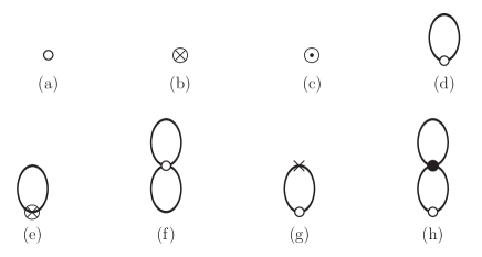
Figure 2: Feynman diagrams up to $p^{6}$ for $\langle\bar{q}q\rangle$.
vertices $\circ$, $\odot$ and $\otimes$ stand for the insertion of $\langle\bar{q}q\rangle$ at $p^{2}$, $p^{2}$ and $p^{6}$ respectively. $\bullet$ is the $p^{2}$ and $\times$ the $p^{4}$ vertices. Solid lines indicates the meson propagator. BGH

At finite volume integration over momenta should be replaced by a summation over discretized momenta. It is also important to note that the pole structure does not change its form, since the singularity arises when momenta in the loop become very large and therefore the pole remains unchanged despite the replacement of integration with summation. The final result for the integrals at finite volume becomes

$$\bar{A}(m^{2}) = -\frac{m^{2}}{16\pi^{2}}\log\left(\frac{m^{2}}{\mu^{2}}\right)$$ (13)

$$-\frac{1}{16\pi^{2}}\sum_{k=1,\infty}x(k)\frac{4m^{2}}{\zeta(k)}K_{1}(\zeta(k))$$

$$\bar{B}(m^{2}) = -\frac{1}{16\pi^{2}}\log\left(\frac{m^{2}}{\mu^{2}}\right)-\frac{1}{16\pi^{2}}$$ (14)

$$+\frac{1}{16\pi^{2}}\sum_{k=1,\infty}x(k)2K_{o}(\zeta(k))$$

with $\zeta(k)=\sqrt{k}mL$. It is evident from equations (13) and (14) that the simple relation $\bar{A}(m^{2})=m^{2}(1/16\pi^{2}+\bar{B}(m^{2}))$ is no longer valid in finite volume computations. After putting all the diagrams together and applying the dimensional regularization scheme with renormalization parameter $\mu$ we ensure that the divergent parts cancel and for finite part we use the expressions in (13) and (14) instead of those in (11) and (12). The parts containing $A^{\epsilon}$ and $B^{\epsilon}$ cancel in the final result for the vacuum expectation value. We denote the lowest order masses for pions, kaons and etas as $\chi_{\pi}$, $\chi_{K}$ and $\chi_{\eta}$ respectively. They are given in terms of the strange quark mass, $m_{s}$ and the average of up quark and down quark masses, $\hat{m}$ by

$$\chi_{\pi}=2B_{0}\hat{m}\,,\quad\chi_{K}=B_{0}(m_{s}+\hat{m})\,$$

$$\chi_{\eta}=2B_{0}(2m_{s}+\hat{m})/3\,.$$ (15)

We also define the following quantities

$$\langle\bar{u}u\rangle = -B_{0}F_{0}^{2}\left(1+\frac{v_{4}^{(u)}}{F_{0}}+\frac{v_{6}^{(u)}}{F_{0}^{2}}\right)\,,$$

$$\langle\bar{s}s\rangle = -B_{0}F_{0}^{2}\left(1+\frac{v_{4}^{(s)}}{F_{0}}+\frac{v_{6}^{(s)}}{F_{0}^{2}}\right)\,.$$ (16)

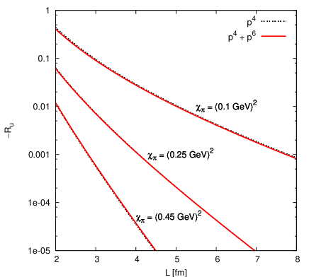
Figure 3: The ratio $R_{u}$ is shown for three different pion massesBGH .

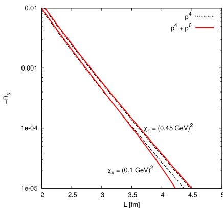
Figure 4: The ration $R_{s}$ is shown for three different pion masses increasing from top to bottom BGH .

The analytical expressions for $v_{4}^{(u)}$,$v_{4}^{(s)}$, $v_{6}^{(u)}$,$v_{6}^{(s)}$ are evaluated in ChPT and can be found in BGH . Numerical results are shown in Fig. 3 and Fig. 4, where the ratio $R_{q}$ is defined as

$$R_{q}\equiv\frac{\langle\bar{q}q\rangle_{V}-\langle\bar{q}q\rangle_{\infty}}{\langle\bar{q}q\rangle_{\infty}}\,.$$ (17)

The $C^{r}_{i}$, the low energy coupling constants (LECs) from diagrams at $p^{6}$ BCE cancel out in the numerator and we have ignored them in the denominator but the $L^{r}_{i}$ will be considered as inputs and we use the values from fit 10 ofABT . As expected the volume size effects are pronounced for small L and small pion mass. But the full NNLO contribution to the finite volume effect is much smaller than the total NNLO numerical correction. In turn this total NNLO correction is smaller than the one presented in ABP . This is due to the fact that in Ref. ABP the physical value of pion decay constant $F_{\pi}$ and also physical masses for mesons are put in the formula.

IV Conclusions

We compared the quark condensate in finite volume obtained in two different ways. The method referred to as Lüscher’s approach yields the leading term of this quantity to all orders in perturbation theory while only one propagator experiences the finite volume. One the other hand, we try to do this computation up to $p^{6}$ rather directly by letting the modification of all propagators be present at the same time. The comparison of the direct calculation at one-loop with the extended formula is trivial but at two-loop level, however, this is not the case. This allows in principle a check of the accuracy of the extended Lüscher approach. Unfortunately, because of the very small size of the finite volume effect at $p^{6}$, no conclusion can be drawn concerning the accuracy level of the extended Lüscher formula from our work.

- (1) S. Weinberg, PhysicaA 96 (1979) 327.
- (2) J. Gasser and H. Leutwyler, Annals Phys. 158 (1984) 142; Nucl. Phys. B 250 (1985) 465.
- (3) J. Bijnens, G. Colangelo and G. Ecker, JHEP 9902 (1999) 020 [arXiv:hep-ph/9902437]; Annals Phys. 280 (2000) 100 [arXiv:hep-ph/9907333].
- (4) J. Gasser and H. Leutwyler, Nucl. Phys. B 307 (1988) 763.
- (5) S. Descotes-Genon, Eur. Phys. J. C 40 (2005) 81 [arXiv:hep-ph/0410233].
- (6) M. Lüscher, Commun. Math. Phys. 104 (1986) 177.
- (7) M. Lüscher, DESY 83/116, Lecture given at Cargese Summer Institute, Cargese, France, 1-15 September 1983.
- (8) G. Colangelo and C. Haefeli, Phys. Lett. B 590 (2004) 258 [arXiv:hep-lat/0403025].
- (9) J. Bijnens and K. Ghorbani, “Finite volume dependence of the quark-antiquark vacuum expectation Phys. Lett. B 636 (2006) 51 [arXiv:hep-lat/0602019].
- (10) G. Colangelo and S. Durr, Eur. Phys. J. C 33 (2004) 543 [arXiv:hep-lat/0311023].
- (11) G. Amorós, J. Bijnens and P. Talavera, Nucl. Phys. B 585 (2000) 293 [Erratum-ibid. B 598 (2001) 665] [arXiv:hep-ph/0003258].
- (12) G. Amorós, J. Bijnens and P. Talavera, Nucl. Phys. B 602 (2001) 87 [arXiv:hep-ph/0101127].