Modified $SO(3)$ Lattice Gauge Theory at $T\neq 0$ with Parallel Tempering:
Monopole and Vortex Condensation

Abstract

The deconfinement transition is studied close to the continuum limit of $SO(3)$ lattice gauge theory. High barriers for tunnelling among different twist sectors causing loss of ergodicity for local update algorithms are circumvented by means of parallel tempering. We compute monopole and center vortex free energies both within the confining phase and through the deconfinement transition. We discuss in detail the general problem of defining order parameters for adjoint actions.

I Introduction

Understanding confinement in $SU(N)$ Yang-Mills theories remains one of the major challenges of contemporary particle physics. Lattice simulations have offered unique insight into the non-perturbative regularization of pure gauge actions transforming under the fundamental representation of $SU(N)$ McLerran and Svetitsky (1981); Kuti et al. (1981), equivalent to the quenched limit of full QCD: at non-zero temperature they have been shown to possess a phase transition linked to the spontaneous breaking of center symmetry Polyakov (1978); Susskind (1979). For $N=2$ it is of second order, therefore lying in the universality class of the 3-d Ising model. However the question whether and in what sense this also holds for discretizations transforming under the natural continuum pure Yang-Mills gauge symmetry group $SU(N)/\mathbb{Z}_{N}$, for $N=2$ equivalent to $SO(3)$, still needs to be appropriately answered Smilga (1994). According to universality Svetitsky and Yaffe (1982), i.e. expecting the different formulations to be equivalent in the continuum limit, they should lead to the same non-perturbative physics. A discretization which does not break the $SU(N)/\mathbb{Z}_{N}$ invariance has moreover the appeal to preserve the topological properties related to $\pi_{1}(SU(N)/\mathbb{Z}_{N})=\mathbb{Z}_{N}$ discussed e.g. in ’t Hooft (1978, 1979); de Forcrand and Jahn (2003).

Since the lattice link variables gauge transform at different points $U_{\mu}(x)\to g^{\dagger}(x)U_{\mu}(x)g(x+\hat{\mu})$, $SU(N)/\mathbb{Z}_{N}$ invariance cannot be recovered from the local cancellation of the $\mathbb{Z}_{N}$ dependence in $g(x)$ as in the continuum and must be imposed directly on $U_{\mu}(x)$. As a consequence in adjoint theories regularized on the lattice it is by construction impossible to define observables transforming under the fundamental representation, i.e. sensitive to the $\mathbb{Z}_{N}$ center of the gauge group: their expectation value will vanish identically irrespective of the dynamics of the theory. Therefore the symmetry breaking arguments for the deconfinement transition mentioned above cannot apply. It remains an open question whether a non-perturbative regularization of Yang-Mills theories allowing both $SU(N)/\mathbb{Z}_{N}$ invariance and non-vanishing fundamental observables can be defined.

In spite of all these interesting problems adjoint actions have not been intensively studied in the literature. For $N=2$ difficulties in their analysis have been well known for a long time Bhanot and Creutz (1981); Greensite and Lautrup (1981); Halliday and Schwimmer (1981a, b): the theory exhibits a bulk transition related to the condensation of $\mathbb{Z}_{2}$ monopole charges $\sigma_{c}=-1$ which hinders the study of its finite temperature properties. First concrete efforts to study the theory at finite temperature by implementing a $\mathbb{Z}_{2}$ monopole suppressing chemical potential, as suggested in Halliday and Schwimmer (1981a, b), were made ten years ago Cheluvaraja and Sharathchandra (1996); Datta and Gavai (1998) reviving the interest in the subject. However, given the absence of a natural order parameter, attempts to locate a transition within phase II (the phase characterized by strong $\mathbb{Z}_{2}$ monopole suppression, see Fig. 1) through thermodynamic observables were only conclusive in the strong coupling region Datta and Gavai (2000, 1999). In these works it was also first observed how in some regions of phase II close to the bulk transition the theory possesses new states where the adjoint Polyakov loop $L_{A}\to-1/3$, additionally to the expected states where $L_{A}\to 1$. In Ref. de Forcrand and Jahn (2003) a dynamical observable measuring the twist expectation value $z$, i.e. the topological index linked to $\pi_{1}(SU(N)/\mathbb{Z}_{N})$, was introduced noting that the $\delta(\sigma_{c}-1)$ constraint effectively implemented by a $\mathbb{Z}_{2}$ monopole suppression should allow the $SO(3)$ partition function to be rewritten as the sum of $SU(2)$ partition functions with all possible twisted boundary conditions $Z|_{z={\rm i}}$, ($i=0,\ldots,3$ for $SU(2)$ on a 3+1 dimensional torus) Mack and Petkova (1982); Tomboulis (1981); Kovacs and Tomboulis (1998); Alexandru and Haymaker (2000). The $L_{A}\to-1/3$ state was thus linked directly to a non-trivial twist expectation value, equivalent to the creation of a vortex. Creating such ’t Hooft loop amounts to changing the signs of some fundamental plaquettes, which however leaves the adjoint action unmodified. This implies that $\Delta U=0$ in the free energy change $\Delta F=\Delta U-T\Delta S$, which will then only receive an entropy contribution. Defining thus the ’t Hooft vortex free energy $F/T=-\log{({Z|_{z=1}}/{Z|_{z=0}})}$ simply by the ratio of the partition function in the non-trivial twist sector to that in the trivial one, their relative weight being measured through an ergodic simulation, the $SO(3)$ theory was proposed as the ideal test case to check whether the ’t Hooft vortex confinement criterion ’t Hooft (1978, 1979) could compensate for the absence of an explicit order parameter linked to center symmetry breaking: in the thermodynamic limit ($V=N_{s}^{3}\to\infty$) $F$ should vanish in the confined phase while diverging with an area law $F\sim\tilde{\sigma}N_{s}^{2}$ above the deconfinement transition. Working without the monopole suppression term proved however to be a hurdle, since the “freezing” of twist sectors above the bulk transition creates high potential barriers hard to overcome even with a multi-canonical algorithm de Forcrand and Jahn (2003), making ergodic simulations on top of the bulk transition unviable already for volumes larger than $8^{3}\times 4$. Furthermore, since one would eventually need to go well beyond the bulk transition deeply into phase II with the simulations, the suitability of multihistogram Swendsen and Wang (1987) or multicanonical methods Berg and Neuhaus (1991) remains dubious. Ergodicity problems and non-trivial twist sectors were not considered in Ref. Datta and Gavai (2000, 1999).

A particular observation has proven crucial in our taming of the tunnelling problem: the bulk transition weakens with increasing $\mathbb{Z}_{2}$ monopole suppression, eventually becoming 2^nd order at some intermediate point Datta and Gavai (2000). Through the twist susceptibility the 2^nd order branch of the bulk transition was shown to be consistent with the 4-d Ising model universality class Datta and Gavai (2000); Barresi et al. (2002, 2003); Barresi and Burgio (2006), as expected by theoretical arguments Halliday and Schwimmer (1981a, b). To actually pin down the point where the transition changes from weak first to second order is a difficult numerical task. This however has no practical consequences, since for the following it is immaterial whether one deals with a second or a very weak first order bulk.

Although tunnelling among topological sectors is still suppressed with a local update algorithm, twists were shown to be well defined throughout phase II. $L_{A}$ on the other hand approximately satisfies Smilga (1994); Michael (1985) a Haar-measure distribution for low $\beta_{A}$, departing from it above some $\beta_{A}^{c}$. The critical value $\beta_{A}^{c}$ was seen to scale properly with the lattice extent in the Euclidean time direction $N_{\tau}$ Barresi et al. (2004a); Barresi and Burgio (2006). This hints at a transition line (the dashed horizontal line in Fig. 1) separating a confining from a deconfining phase in each fixed twist sector Barresi et al. (2004a, b, c); Barresi and Burgio (2006) collapsing on the bulk transition for the $N_{\tau}$ commonly used in simulations. It is therefore sound to conjecture that the whole physically relevant $SO(3)$ dynamics lies in phase II, the finite temperature transition eventually decoupling from the bulk transition for high enough $N_{\tau}$ even without monopole suppression term. Unfortunately, according to estimates in Ref. de Forcrand and Jahn (2003) this should not happen for lattice sizes smaller than $\sim 800^{3}\times 400$. A non-vanishing $\mathbb{Z}_{2}$ monopole chemical potential together with an ergodic algorithm suitable for simulations throughout phase II seems therefore the only feasible way to gain access to the properties of the continuum limit of $SO(3)$.

Given the failure of center symmetry breaking criteria to identify the deconfinement transition in the adjoint theory, in Barresi et al. (2004d); Barresi and Burgio (2006) the use of the Pisa disorder parameter for monopole condensation was proposed. Lines of second order transition properly scaling with $N_{\tau}$ and ending on the bulk transition line where actually found at fixed twist, with critical exponents consistent with the 3-d Ising model. Whether this is the case also for the ergodic theory, i.e. summed over all twist sectors, is the subject of the present paper. We will employ parallel tempering and utilize the mentioned weakening of the bulk transition to overcome the high potential barriers that prevent tunnelling with local update algorithms. Moreover, ergodicity being an essential prerequisite for an unbiased measure of the vortex free energy, it is an interesting question in its own right whether such observable could indeed also play the rôle of an order parameter for the deconfinement transition in $SO(3)$ de Forcrand and Jahn (2003); de Forcrand and von Smekal (2002). We will extend here the discussion of the vortex free energy we have recently published in Ref. Burgio et al. (2006a). Some preliminary results of the present project were also presented in Burgio et al. (2006b).

II The setup and the observables

As anticipated, we will concentrate on the adjoint $SU(2)$ Wilson action modified by a $~{}\mathbb{Z}_{2}$ monopole suppression term

$$S=\beta_{A}\sum_{P}\left(1-\frac{1}{3}\mathrm{Tr}_{A}U_{P}\right)+\lambda\sum_{c}(1-\sigma_{c})\,,$$ (1)

where $U_{P}$ denotes the standard plaquette variable and $\mathrm{Tr}_{A}O=(\mathrm{Tr}_{F}O)^{2}-1=\mathrm{Tr}_{F}(O^{2})+1$ the adjoint trace. The center blind product $\sigma_{c}=\prod_{P\in\partial c}\mathrm{sign}(\mathrm{Tr}_{F}U_{P})$ taken around elementary 3-cubes $c$ defines the $\mathbb{Z}_{2}$ magnetic charge. Its density $M=1-\langle\frac{1}{N_{c}}\sum_{c}\sigma_{c}\rangle$ tends to unity in the strong coupling region (phase I) and to zero in the weak coupling limit (phase II), $N_{c}$ denoting the total number of elementary 3-cubes. The corresponding path-integral quantized lattice theory with the action (1) is center-blind in the entire $\beta_{A}-\lambda$ plane Barresi et al. (2004a).

The Pisa disorder parameter $\mu$ Di Giacomo and Paffuti (1997); Di Giacomo et al. (2000a, b); Carmona et al. (2001) has been introduced for action (1) in Ref. Barresi et al. (2004d). Its expectation value is given by $\langle\mu\rangle=\langle e^{-\Delta S}\rangle$, where $\Delta S=S^{M}-S$ is the difference of the standard plaquette action $S$ and an action $S^{M}$ modified by the introduction of an adjoint bosonic field transforming at the space boundary under $G\sim SU(2)/U(1)$ Di Giacomo and Paffuti (1997); Fröhlich and Marchetti (2001). Its evaluation does not require any gauge fixing, a point of view we adopt in what follows Fröhlich and Marchetti (2001). We want to stress here that the introduction of $C^{*}$ boundary conditions in the temporal direction, necessary to conserve magnetic charge when defining $S^{M}$ at finite temperature, poses no conceptual problem in the adjoint theory, being equivalent up to a gauge rotation to a partial twist, i.e. only in the time direction Barresi et al. (2004d). Since our adjoint action with periodic boundary conditions allows all twist matrices to be generated dynamically in any direction de Forcrand and Jahn (2003), $C^{*}$ boundary conditions will just amount to a relabelling of the twist sectors. We will come back to this point later on.

Appropriate twist variables are introduced by de Forcrand and Jahn (2003)

$$z_{\mu\nu}\equiv\frac{1}{N_{\rho}N_{\sigma}}\sum_{\rho\sigma}\prod_{P\;\in\;\mathrm{plane}\;\mu\nu}\!\!\mathrm{signTr}_{F}U_{P}\,,\hskip 2.84544pt(\epsilon_{\rho\sigma\mu\nu}=1).$$ (2)

Since the temporal twists in the various spatial directions $z_{i,4}\,,i=1,2,3$ are well identified (either +1 or -1) for each configuration in phase II, the partition functions restricted to a fixed twist sector are easy to define as expectation values of suitable projectors ’t Hooft (1979). Explicitly we have

$${\frac{Z|_{z=0}}{Z}}=\langle\nu_{0}\rangle,\;\;\; \nu_{0} ={\frac{1}{8}}\prod_{i=1}^{3}[1+\mathrm{sign}(z_{i,4})]$$

$${\frac{Z|_{z=1}}{Z}}=\langle\nu_{1}\rangle,\;\;\; \nu_{1} ={\frac{1}{8}}\sum_{j=1}^{3}\;\prod_{i=1}^{3}[1+(1-2\delta_{i,j})\mathrm{sign}(z_{i,4})]$$

$${\frac{Z|_{z=2}}{Z}}=\langle\nu_{2}\rangle,\;\;\; \nu_{2} ={\frac{1}{8}}\sum_{j=1}^{3}\;\prod_{i=1}^{3}[1-(1-2\delta_{i,j})\mathrm{sign}(z_{i,4})]$$

$${\frac{Z|_{z=3}}{Z}}=\langle\nu_{3}\rangle,\;\;\; \nu_{3} ={\frac{1}{8}}\prod_{i=1}^{3}[1-\mathrm{sign}(z_{i,4})]$$ (3)

$\nu_{k}$ being equal to unity if the configuration belongs to the $k^{\rm th}$ sector and vanishing otherwise.

From Eq. (3) it follows that

$$F=-T\log{{\frac{Z_{1}}{3Z_{0}}}}=-{\frac{1}{aN_{\tau}}}\log{{\frac{\langle\nu_{1}\rangle}{3\langle\nu_{0}\rangle}}}\,.$$ (4)

The factor in the denominator is due to the three equivalent ways to measure $z_{i,4}=-1$ on $\mathbb{T}^{3}\times\mathbb{S}$, rather than one as on $\mathbb{S}^{3}\times\mathbb{S}$; in this way $F$ will be normalized to zero if 0- and 1-twists are equally probable. This occurs on top of the bulk transition and in some sense everywhere in phase I, where twist sectors are however badly defined, because of the twist variables (2) fluctuating around zero.

We will employ parallel tempering to achieve ergodicity over different twist sectors when evaluating the expectation values of physical observables, e.g. the Pisa disorder parameter and the ’t Hooft vortex free energy. Simulations have been carried out along the paths shown in Fig. 1.

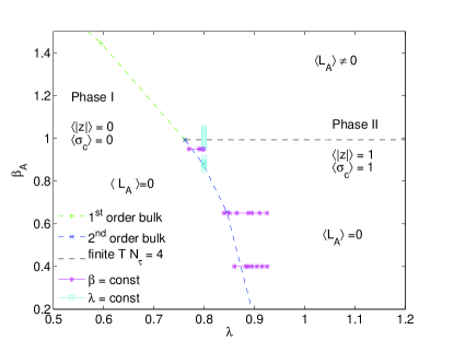
Figure 1: Paths chosen for main simulations in the $\lambda-\beta_{A}$ plane.

The motivation for these choices will become clear in the following. Our spatial lattice sizes will vary between $N_{s}=12$ and $N_{s}=24$. The time-like extension will remain fixed ($N_{\tau}=4$).

III Parallel tempering

III.1 General description

In tempering methods some parameters of the action are made dynamical variables in the simulations, updating the system in an enlarged configuration space. This allows a detour in parameter space if a high tunnelling barrier is present at some parameter value, resulting in an improved algorithm.

In the method of simulated tempering first proposed in Marinari and Parisi (1992) the inverse temperature is made a dynamical variable. With such algorithms considerable improvements have been obtained when rendering dynamical e.g. the number of degrees of freedom in the Potts-Model Kerler and Weber (1993), the inverse temperature for spin glass Kerler and Rehberg (1994) and the monopole coupling in U(1) lattice theory Kerler et al. (1994, 1995). With dynamical mass of staggered fermions in full QCD Boyd (1996) a better sampling of the configuration space has been reported. However, simulated tempering requires the determination of a weight function in the generalized action, and an efficient method of estimating it Kerler and Rehberg (1994); Kerler et al. (1994, 1995) is crucial for successfully accelerating the simulation.

A major progress was the proposal of the parallel tempering method (PT) Hukushima and Nemoto (1995); Marinari (1996), in which no weight function needs to be determined. This method has allowed great improvements for spin glasses Hukushima and Nemoto (1995). In QCD with dynamical quark mass better sampling has been reported for staggered fermions Boyd (1998). In simulations of QCD with O($a$)-improved Wilson fermions Joo et al. (1999) no computational advantage has been found when making only two (relatively small) hopping parameter values dynamical. In subsequent works Ilgenfritz et al. (2000a, b) with more ensembles and standard Wilson fermions a considerable increase of the transitions between topological sectors has been observed. In Ref. Ilgenfritz et al. (2002) these investigations have been extended to a detailed comparison with conventional simulations. Unfortunately no gain could be confirmed in that case due to the region of parameter space used in which the mechanism of an easier detour was not available.

In the present application the fact that above the bulk phase transition the barriers between the twist sectors cannot be overcome at all by conventional algorithm makes PT in any case superior. With a chain of parameter points crossing the transition line along the softer branch of the bulk transition the idea of an easier detour by tempering is ideally realized. This is also reflected by the remarkably good efficiency of PT observed.

III.2 Parallel tempering algorithm

In standard Monte Carlo simulations one deals with one parameter set $p$ and generates a sequence of field configurations ${\cal{}_{F}}(s)$, where $s$ denotes the Monte Carlo time. In our case $p$ will include the coupling $\beta_{A}$ and the chemical potential $\lambda$. In parallel tempering (PT) Hukushima and Nemoto (1995); Marinari (1996) one updates $K$ field configurations ${\cal{}_{F}}_{n}$ with $n=1,\dots,K$ in the same run. The characteristic feature is that the assignment of the parameter sets $p_{j}$ with $j=1,\dots,K$ to the field configurations ${\cal{}_{F}}_{n}$ changes in the course of a tempered simulation. The global configuration at time $s$ will be denoted by $B(s)$, ${\cal{}_{F}}_{1}(s)$, ${\cal{}_{F}}_{2}(s)$,…, ${\cal{}_{F}}_{K}(s)$ where the permutation

$$B(s)=\left(\begin{array}[]{cccccc}n_{1}(s)&n_{2}(s)&\ldots&n_{j}(s)&\ldots&n_{K}(s)\\ 1&2&\ldots&j&\ldots&K\\ \end{array}\right)$$ (5)

describes the assignment of the field configurations ${\cal{}_{F}}_{n_{j}(s)}(s)$ to the parameter sets $p_{j}$. For short this approach is called PT with $K$ ensembles.

The update of the ${\cal{}_{F}}_{n}$ is implemented through a standard Metropolis procedure using the parameter sets $p_{j}$ as assigned at a given time. The update of $B$ is achieved by swapping pairs according to a further Metropolis acceptance condition with probability

$$P_{\rm swap}(i,j)=\min\left(1,e^{-\Delta S}\right)\,,$$ (6)

where the variation

$$\Delta S= + S(p_{i},{\cal{}_{F}}_{n_{i}})+S(p_{j},{\cal{}_{F}}_{n_{j}})$$ (7)

$$- S(p_{i},{\cal{}_{F}}_{n_{j}})-S(p_{j},{\cal{}_{F}}_{n_{i}})$$

refers to the action $S$ for the parameter set $p_{j}$ and the field configurations ${\cal{}_{F}}_{n_{j}}$. The total update of the Monte Carlo algorithm, after which its time $s$ increases by one, then consists of the updates of all ${\cal{}_{F}}_{m}$ followed by the full update of $B$ with a sequence of attempts to swap pairs.

Detailed balance for the swapping follows from Eq. (7). Ergodicity is obtained by updating all ${\cal{}_{F}}_{n}$ and by swapping pairs in such a way that all permutations of Eq. (5) can be reached. There remains still the freedom of choosing the succession of the individual steps. Our choice is such that the updates of all ${\cal{}_{F}}_{n}$ and that of $B$ alternate. Our criterion for choosing the succession of swapping pairs in the update of $B$ has been to minimize the average time it takes for the assignment of a field configuration to the parameters to travel from the first to the last pair of parameter values. This has led us to swap neighboring pairs and to proceed with this along the respective path in Fig. 1.

Observables of interest, associated to a specific set $p_{j}$, will be denoted as

$$\mathcal{O}_{j}(s)\equiv\mathcal{O}({\cal{}_{F}}_{n_{j}(s)}(s)),\quad j=1,\ldots,K\,.$$ (8)

As anticipated above, for the success of the method the softening of the bulk transition is crucial, since we need to “transport” the tunnelling that occurs in phase I and on top of the bulk transition into phase II, where twist sectors are well defined but frozen. To work at low $\lambda$, i.e. on top of a strong 1^st order bulk, would select too high barriers and kill any hope of ergodicity at large volume, as experienced in Ref. de Forcrand and Jahn (2003); de Forcrand and von Smekal (2002). Moreover, in that parameter range for lattice sizes reasonably available to the simulations (i.e. $\ll 800^{3}\times 400$!) finite volume effects would still cover the physical transition de Forcrand and Jahn (2003).

Some care is of course necessary also with our method. In particular to maintain a sufficient swapping acceptance rate $\omega$, i.e. to avoid the freezing of twist sectors, the distance between neighboring couplings must diminish with the volume. On the other hand to keep cross-correlations under control one does not wish the acceptance rate to be too high. We have chosen to tune the parameters for each path and volume at hand so to keep the acceptance rate roughly fixed at around $\omega=12\%$, a value for which we empirically find a good balance between auto- and cross-correlations. We also find that performing some standard Metropolis overupdate hits on the ${\cal{}_{F}}_{n}$ before the actual PT update (7) is proposed helps in diminishing correlations.

The relatively low value of $\omega$ has an intuitive explanation: for each parameter set $p_{j}$ one wishes to “explore” the various twist sectors for a sufficiently long MC time before tunnelling. It causes however also a technical problem: if the starting configurations are all in the same twist sector the ensemble needs a very long time before the “disorder” below the bulk spreads to the configurations further above it. An efficient way out is to randomly choose the twist sectors of the elements in the start ensemble.

$N_{s}=12$		$N_{s}=16$		$N_{s}=20$(a)		$N_{s}=20$(b)
$2\times 40000$		$2\times 40000$		$2\times 40000$		$2\times 40000$
$\lambda$	$\beta_{A}$	$\lambda$	$\beta_{A}$	$\lambda$	$\beta_{A}$	$\lambda$	$\beta_{A}$
0.78	0.960	0.78	0.960	0.77	0.960	0.77	0.960
0.79	0.960	0.79	0.960	0.78	0.960	0.78	0.960
0.80	0.960	0.80	0.960	0.79	0.960	0.79	0.960
0.80	0.975	0.80	0.970	0.80	0.960	0.80	0.960
0.80	0.990	0.80	0.981	0.80	0.970	0.80	0.970
0.80	1.005	0.80	0.993	0.80	0.980	0.80	0.980
0.80	1.020	0.80	1.006	0.80	0.990	0.80	0.990
0.80	1.035	0.80	1.019	0.80	1.000	0.80	1.005
0.80	1.050	0.80	1.032	0.80	1.010	0.80	1.015
0.80	1.065	0.80	1.045	0.80	1.025	0.80	1.035
0.80	1.080	0.80	1.058	0.80	1.040	0.80	1.045
0.80	1.090	0.80	1.070	0.80	1.050	0.80	1.055

Table 1: Lattice sizes, statistics and couplings for PT simulations in Fig. 7 and Fig. 8, right branch.

$N_{s}=12$		$N_{s}=16$		$N_{s}=20$
$2\times 40000$		$2\times 40000$		$2\times 40000$
$\lambda$	$\beta_{A}$	$\lambda$	$\beta_{A}$	$\lambda$	$\beta_{A}$
0.80	0.860	0.80	0.860	0.80	0.860
0.80	0.870	0.80	0.870	0.80	0.870
0.80	0.875	0.80	0.880	0.80	0.875
0.80	0.880	0.80	0.890	0.80	0.880
0.80	0.885	0.80	0.895	0.80	0.885
0.80	0.890	0.80	0.900	0.80	0.890
0.80	0.900	0.80	0.908	0.80	0.895
0.80	0.905	0.80	0.920	0.80	0.908
0.80	0.908	0.80	0.925	0.80	0.925
0.80	0.910
0.80	0.920
0.80	0.925

Table 2: Parameter sets for PT runs in Fig. 8, left branch.

$N_{s}=12$		$N_{s}=16$		$N_{s}=20$
$30000$		$30000$		$30000$
$\lambda$	$\beta_{A}$	$\lambda$	$\beta_{A}$	$\lambda$	$\beta_{A}$
0.80	0.865	0.80	0.865	0.80	0.865
0.80	0.870	0.80	0.870	0.80	0.870
0.80	0.875	0.80	0.875	0.80	0.875
0.80	0.880	0.80	0.880	0.80	0.880
0.80	0.890	0.80	0.890	0.80	0.890
0.80	0.900	0.80	0.900	0.80	0.900
0.80	0.910	0.80	0.910	0.80	0.910
0.80	0.920	0.80	0.920	0.80	0.920
0.80	0.930	0.80	0.930	0.80	0.930
0.80	0.935	0.80	0.935	0.80	0.935

Table 3: Parameters sets for PT runs in Fig. 9, left branch.

$N_{s}=12$		$N_{s}=16$		$N_{s}=20$		$N_{s}=24$
$100000$		$100000$		$100000$		$100000$
$\lambda$	$\beta_{A}$	$\lambda$	$\beta_{A}$	$\lambda$	$\beta_{A}$	$\lambda$	$\beta_{A}$
0.78	0.95	0.78	0.95	0.785	0.95	0.785	0.95
0.79	0.95	0.79	0.95	0.795	0.95	0.795	0.95
0.795	0.95	0.795	0.95	0.7975	0.95	0.7975	0.95
0.80	0.95	0.80	0.95	0.80	0.95	0.80	0.955
0.80	0.96	0.80	0.96	0.80	0.96	0.80	0.960
0.80	0.97	0.80	0.97	0.80	0.967	0.80	0.966
0.80	0.98	0.80	0.98	0.80	0.974	0.80	0.972
0.80	0.99	0.80	0.99	0.80	0.981	0.80	0.978
0.80	1.00	0.80	1.00	0.80	0.988	0.80	0.984
0.80	1.01	0.80	1.01	0.80	0.995	0.80	0.991
0.80	1.02	0.80	1.02	0.80	1.002
0.80	1.03	0.80	1.03	0.80	1.009
0.80	1.04	0.80	1.04	0.80	1.016
0.80	1.05	0.80	1.05	0.80	1.023

Table 4: Parameters sets for PT runs in Fig. 9, right branch.

$N_{s}=12$		$N_{s}=16$		$N_{s}=20$
$100000$		$100000$		$100000$
$\lambda$	$\beta_{A}$	$\lambda$	$\beta_{A}$	$\lambda$	$\beta_{A}$
0.80	0.92	0.80	0.92	0.80	0.932
0.80	0.93	0.80	0.93	0.80	0.939
0.80	0.94	0.80	0.94	0.80	0.946
0.80	0.95	0.80	0.95	0.80	0.953
0.80	0.96	0.80	0.96	0.80	0.960
0.80	0.97	0.80	0.97	0.80	0.967
0.80	0.98	0.80	0.98	0.80	0.974
0.80	0.99	0.80	0.99	0.80	0.981
0.80	1.00	0.80	1.00	0.80	0.988
0.80	1.01	0.80	1.01	0.80	0.995
0.80	1.02	0.80	1.02	0.80	1.002
0.80	1.03	0.80	1.03	0.80	1.009
0.80	1.04	0.80	1.04	0.80	1.016
0.80	1.05	0.80	1.05	0.80	1.023

Table 5: Parameter sets for PT runs in Figs. 6 and 11.

$N_{s}=16$		$N_{s}=16$
$30000$		$30000$
$\lambda$	$\beta_{A}$	$\lambda$	$\beta_{A}$
0.870	0.40	0.830	0.65
0.883	0.40	0.850	0.65
0.888	0.40	0.865	0.65
0.895	0.40	0.888	0.65
0.905	0.40	0.895	0.65
0.915	0.40	0.910	0.65
0.925	0.40	0.925	0.65

Table 6: Parameter sets for two of the parallel tempering runs in Fig. 10.

Details for the investigated lattice sizes, the chosen parameter sets $~{}(\lambda,\beta_{A})_{j},~{}j=1,2,\ldots,K~{}$ and the statistics for each ensemble for the paths drawn in Fig. 1 are listed in the columns of Tables 1 to 6. Remember that the path along which we are passing through the finite temperature transition at fixed $~{}\lambda=0.8~{}$ starts with a horizontal piece at fixed $\beta_{A}=0.95$. The factor 2 for $N$ in Tables 1 and 2 refers to the runs with and without modified action $S^{M}$, respectively. In order to remain on the safe side in some results we have omitted the first and last elements of the ensembles, since the latter have no further configuration to swap with. The respective errors of these points might not be of a comparable quality. In the literature one can find that by adjusting the parameter spacing such that the endpoints get visited with the same probability as the neighboring points the errors tend to become comparable.

For the fixed $\lambda$ path of Fig. 1, along which the main simulations have been performed, we can fit very well the step $~{}\delta\beta_{A}~{}$ needed to keep $~{}\omega~{}$ fixed with a scaling law of the form

$$\delta\beta_{A}(\omega,N_{s})\simeq\frac{\alpha(\omega)}{N_{s}^{2}}\,,$$ (9)

where we find $\alpha(12\%)=2.15(3)$ in the $\beta_{A}=0.95-1.09$ range considered, although we expect it to change with the width and location of the the $(\lambda,\beta_{A})$ window. Being $\omega$ nothing but the tunneling probability among twist sectors, it should be proportional to the probability to create a vortex. Since the cost to generate the latter should scale with an area law ’t Hooft (1979), the $N_{s}^{2}$ dependance of the former is easily understood. Eq. (9) implies that to explore a fixed region $\Delta\beta_{A}$ of parameter space the number of ensembles will scale like

$$K\simeq\frac{\Delta\beta_{A}}{\alpha}N_{s}^{2}$$ (10)

As an illustration of the ergodicity of the algorithm we show in Fig. 2 the MC time histories of the twist observables $z_{i,4}$ and of the adjoint Polyakov loop for two ensembles belonging to the same test PT simulation with $K=10$ and $N_{s}=16$, one below (phase I) and one above the bulk transition (phase II). We have first let the single ensembles evolve separately with standard Metropolis updates, i.e. not updating the permutation table $B$. The barriers among sectors are huge de Forcrand and Jahn (2003) and practically impossible to overcome without PT within phase II: the system is simply stuck in a fixed topological sector. Indeed, as Fig. 2 shows the twist variables remained stable over 6000 sweeps until we have turned on the full PT updates. The system started then frequently to tunnel among all sectors. Actually below the bulk transition there is no substantial difference between the two algorithms, since the disorder induced by the $\mathbb{Z}_{2}$ monopoles lets any algorithm be ergodic for the simple reason that topological sectors are ill-defined, all twist values fluctuating around zero. The difference is however dramatic above the bulk transition in phase II, where tunnelling among well-defined topological sectors is enabled by the PT algorithm.

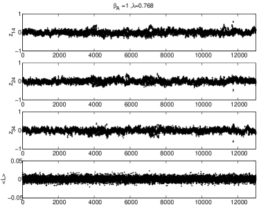
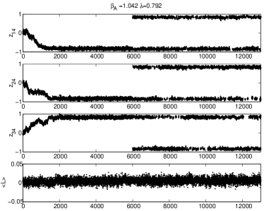
Figure 2: MC histories of twist variables $~{}z_{i,4},~{}i=1,2,3~{}$ and of the adjoint Polyakov loop $~{}L_{A}~{}$ for two PT ensembles. The lattice size is $16^{3}\times 4$.

III.3 Cross and autocorrelations

In PT the $K$ ensembles are generated in a correlated way. Therefore, the full non-diagonal covariance matrix for the observables has to be taken into account. The latter is obtained from the general correlation functions which, for an observable $\mathcal{O}$ and a number $N$ of updates, are defined as

$$R_{jk}(t) = \frac{1}{N}\sum_{s=1}^{N}\mathcal{O}_{j}(s)\mathcal{O}_{k}(s+t)$$ (11)

$$- \Big{(}\frac{1}{N}\sum_{s^{\prime}=1}^{N}\mathcal{O}_{j}(s^{\prime})\Big{)}\Big{(}\frac{1}{N}\sum_{s^{\prime\prime}=1}^{N}\mathcal{O}_{k}(s^{\prime\prime})\Big{)}\,.$$

For $j=k$ they are the usual autocorrelation functions, while for $j\neq k$ they describe cross correlations between different ensembles.

The covariance matrix is obtained Ilgenfritz et al. (2002) by using the general correlation function of Eq. (11) and generalizing the derivation in Ref. Priestley (1989) for the case $j=k$, which gives

$$C_{jk} = \frac{1}{N}R_{jk}(0)$$ (12)

$$+ \frac{1}{N}\sum_{t=1}^{N-1}\Big{(}1-\frac{t}{N}\Big{)}\Big{(}R_{jk}(t)+R_{kj}(t)\Big{)}\,.$$

The diagonal elements of Eq. (12) are the variances of $\mathcal{O}_{j}$ usually written as

$$\mbox{var}(\mathcal{O}_{j})=\frac{R_{jj}(0)}{N}\;2\tau_{j}\;,$$ (13)

with the integrated autocorrelation times $\tau_{j}$

$$\tau_{j}=\frac{1}{2}+\sum_{t=1}^{N-1}\rho_{j}(t),\qquad\rho_{j}(t)=R_{jj}(t)/R_{jj}(0).$$ (14)

When evaluating $\tau_{j}$ according to Eq. (14) in practical simulations the summation up to $N-1$ makes no sense since $\rho_{j}(t)$ is buried in the Monte Carlo noise already for relatively small $t$. Therefore, it has been proposed Priestley (1989); Madras and Sokal (1988) to sum up only to some smaller value $M$ of $t$. However, in practice such procedure is not stable against the choice of $M$ and neglecting the rest is a bad approximation. The proposal to estimate the remainder by an extrapolation based on the $t$-values $M$ and $M-1$ Wolff (1989) is still inaccurate in general. A more satisfying procedure is to describe the rest by a fit function based on the (reliable) terms of Eq. (12) for $t\leq M$ and on the general knowledge about the Markov spectrum. This procedure has led to very good results results in other applications Kerler (1993a).

In order to apply the latter strategy to determine the off-diagonal entries in Eq. (12) one has to study how spectral properties enter the problem. This is possible introducing an appropriate Hilbert space Madras and Sokal (1988); Kerler (1993b). Working this out, in Ref. Ilgenfritz et al. (2002) the general representation

$$R_{jk}(t)=\sum_{r>1}a_{jkr}\gamma_{r}^{t}\quad\mbox{with}\quad|\gamma_{r}|<1$$ (15)

has been obtained, where only the coefficients $a_{jkr}$ depend on the particular pair of observables while the eigenvalues $\gamma_{r}$ are universal and characteristic for the simulation algorithm. To explain the behaviour of the off-diagonal elements the approximate functional form

$$R_{jk}(t)\approx\left\{\begin{array}[]{cl}\sum_{r>1}\tilde{a}_{jkr}\gamma_{r}^{t}&\mbox{for}\quad|j-k|\leq t\\ 0&\mbox{for}\quad 0\leq t<|j-k|\end{array}\right\}$$ (16)

has been derived Ilgenfritz et al. (2002) for $j\neq k$, which indicates a maximum at $t=|j-k|$.

For the numerical evaluation of Eq. (12) the method mentioned above is to be used, generalizing it to the off-diagonal elements. The fits in the noisy region can exploit the universality of the Markov spectrum and the fact that after some time only the slowest mode survives. Of course, such evaluation is limited by the available statistics. To calculate errors one has to account for the cross correlations between the ensembles. To be able to do this one has to rely on fits to the data. The respective fit method is well know from the treatment of indirect measurements (see e.g. Ref. Brandt (1976)). For the application to PT the details have been worked out in Ref. Ilgenfritz et al. (2002). To obtain errors for the covariances one can generalize the derivations given in Ref. Priestley (1989) for the diagonal case to calculate covariances of covariances from the $R_{jk}(t)$ data only. However, in practice one can hardly get enough statistics for this.

III.4 Correlation results

Typical examples of correlation functions $R_{jk}(t)$ (normalized to $R_{jj}(0)$) are shown in Fig. 3, 4 and 5 for the twist variable $z_{1,4}$ as introduced in Section 2.

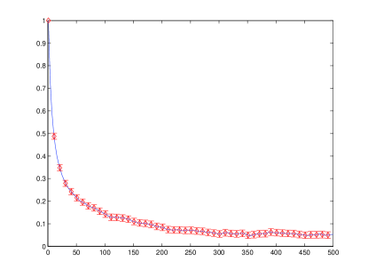
Figure 3: Example of a normalized diagonal correlation function for $z_{1,4}$ at $\beta_{A}=0.98$ and $\lambda=0.8$ on a $16^{3}\times 4$ lattice.

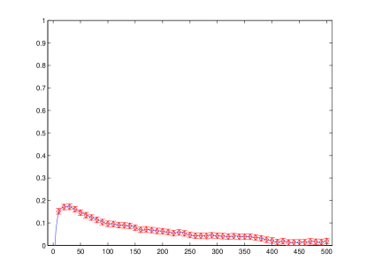
Figure 4: Example of a first off-diagonal normalized correlation function for $z_{1,4}$ between ensembles taken at $\beta_{A}=0.98$ and $0.99$ for $\lambda=0.8$ and lattice size $16^{3}\times 4$.

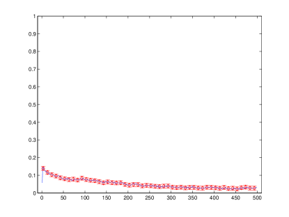
Figure 5: Example of a second off-diagonal normalized correlation function for $z_{1,4}$ between ensembles taken at $\beta_{A}=0.98$ and $1.00$ for $\lambda=0.8$ and lattice size on $16^{3}\times 4$.

Along with all $z_{i,4}$ we have also used the autocorrelations for the Polyakov loop as an additional source to determine the eigenvalues $\gamma_{r}$ in our analysis. For the off-diagonal elements $R_{jk}(t)$ which show a clear signal above the noise we generally observe a maximum at roughly $t=|j-k|$, thus seeing indeed the behaviour predicted by Eq. (16) (within errors) in our data. It is usually difficult to identify more than two or three off-diagonals above the noise. The correlations tend moreover to decrease with increasing volume. From our data we can clearly conclude that the off-diagonal elements of the general correlation functions are decreasing with the distance from the diagonal, their contributions being reasonably smaller than the diagonal one, indicating that cross correlations do not play an essential rôle.

Fig. 6 shows the integrated autocorrelation times for all twist variables $~{}z_{i,4}$ obtained at different volumes for each parallel configuration along the paths at $\lambda=0.8$ in Fig. 1. Autocorrelations clearly decrease with the volume, as expected. As we shall see, the two peaks correspond to the bulk transition and the finite-temperature transition.

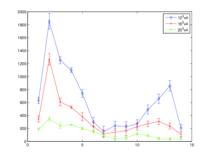
Figure 6: Integrated autocorrelation times for the twist variable $z_{i4}$ at different volumes. The numbers at the horizontal axis enumerate the parameter points $(\lambda,\beta_{A})$ for the PT ensembles corresponding to Tab. 4.

The observables that will suffer most from correlations in PT are obviously those whose expectation value depends significantly on twist sectors. In our practical case only the twists themselves and the vortex free energy are sensitive to the ergodicity properties of the algorithm. For such observables errors will be given by a combination of statistical errors, estimated by bootstrapped sampling, and auto/cross-correlation errors given by error propagation of the errors on $\nu_{i}$. Other observables, like the Polyakov loop and the Pisa disorder parameter, are roughly twist independent away from the deep deconfined phase, which we anyway do not reach in our simulations Barresi et al. (2004d); Barresi and Burgio (2006). For them only the statistical errors will be relevant.

IV Results

IV.1 Monopole condensation

The computation of the Pisa order parameter $\mu$ can be extended to the parallel tempering approach in a straightforward way. Fig. 7 shows $\rho=\frac{d}{d\beta_{A}}\log\langle\mu\rangle$ for fixed $\lambda=0.8$. As discussed in Ref. Barresi et al. (2004d), to prove confinement through monopole condensation $\rho$ should be small and bounded from below in the confined phase, display a dip at the deconfinement transition and reach a negative plateau whose value should scale like $-O(N_{s}\log{N_{s}})$ in the deep deconfined phase.

The dip in Fig. 7 shows the position of the finite temperature transition. The region left to it, where $\rho$ should roughly vanish, is too close to the bulk transition to approach its $\beta_{A}\to 0$ value. $\rho$ indeed has a dip at the bulk transition, as shown in Fig. 8 Barresi et al. (2004d); Barresi and Burgio (2006), where $\mathbb{Z}_{2}$ monopoles disappear. Both phases left and right of the bulk transition are however still confining as long as $\rho$ remains bounded from below on both sides Barresi and Burgio (2006).

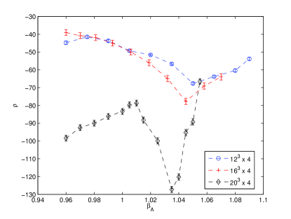
Figure 7: $\rho$ vs. $\beta_{A}$ for $\lambda=0.8$ and various lattice sizes.

Fig. 8 compares the occurrence of the second $\rho$-dip around $\beta_{A}\simeq 0.9$ with the existence of a corresponding peak in the susceptibility of the average twist as defined in Barresi et al. (2004a). While the location of the latter peak is temperature-independent, its height cannot be used to get the scaling with the 4-d volume since this should be calculated at $T=0$. For the susceptibility the latter can be done, obtaining critical exponents in accordance with Ising 4-d, as in Barresi et al. (2004a). On the other hand, the Pisa disorder operator definition we use makes only sense at $T\neq 0$ (for a definition at $T=0$ see Di Giacomo and Paffuti (1997)).

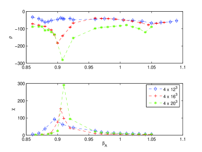
Figure 8: Comparison between the Pisa order parameter $\rho$ (up) and the susceptibility of the average twist $\chi_{z}$ (below) as a function of $\beta_{A}$ for $\lambda=0.8$.

Some caution is therefore necessary in interpreting the results of Fig. 7. The region we investigate is, by the above exposed limitations of the algorithm, very close to both the bulk transition and the physical phase transition, so that two competing effects are superimposing. A thorough analysis of the whole phase space would be very expensive in terms of computer time and could anyway hardly be extended to very high $\beta_{A}$. Nevertheless, as argued in Ref. Barresi and Burgio (2006), from the fixed twist dynamics of our model Barresi et al. (2004d); Barresi and Burgio (2006) one can conclude that for the ergodic theory the Pisa disorder parameter indicates condensation of monopoles in the low $\beta_{A}$ region and deconfinement at high $\beta_{A}$, provided that a diverging dip at some $\beta_{A}^{c}$ exists, as Fig. 7 clearly shows.

Indeed, given that the ergodic expectation value of $\mu$ can be written as

$$\langle\mu\rangle_{erg}=\frac{\sum_{\sf i}\mu|_{z={\sf i}}Z_{\sf SO(3)}|_{z={\sf i}}}{\sum_{\sf i}Z_{\sf SO(3)}|_{z={\sf i}}}\,,$$ (17)

at large $\beta_{A}$, taking into account the observed $O(-N_{s}\log{N_{s}})$ plateaus of $\rho$ for trivial twist and its vanishing at non-trivial twist Barresi et al. (2004d); Barresi and Burgio (2006) we have $\langle\mu\rangle_{erg}\simeq\langle\mu\rangle|_{z=0}(1-e^{-\frac{F}{T}})$. The latter equation clearly implies an exponential vanishing of $\langle\mu\rangle_{erg}$ in the thermodynamic limit at high $\beta_{A}$.

At low $\beta_{A}$ one actually needs a bit more care. In all twist sectors $\rho$ assumes a small constant, bounded from below negative value $\rho\to-\kappa\simeq-10$ Barresi et al. (2004d); Barresi and Burgio (2006), therefore indicating $\langle\mu\rangle\neq 0$ also for the full ergodic theory, i.e. condensation of monopoles and confinement below $\beta^{c}_{A}$ Barresi et al. (2004d). For every fixed $N_{\tau}~{}$ $\langle\mu\rangle_{erg}$ can be rescaled post-hoc to one through $exp(\kappa\beta_{A}^{c}(N_{\tau}))$. This rescaling factor will necessarily diverge for $SU(N)$, up to logarithmic corrections, like $N_{\tau}^{\epsilon\kappa}$ with $\epsilon=2\beta_{0}(N^{2}-1)/N$, $\beta_{0}=11N/(48\pi^{2})$ being the first coefficient of the $\beta$-function. For $SU(2)$ $\epsilon\kappa\simeq 1.4$. This is of course not an obstacle in normalizing $\langle\mu\rangle_{erg}=1$ in the limit $N_{\tau}\to\infty$, although it remains a somewhat inelegant feature of the Pisa disorder operator in the adjoint formulation. There is however a physical motivation for the non vanishing of $\rho$, as we will see in the following.

IV.2 Vortex free energy

Having established the physical properties of phase II at finite temperature, we will now turn to the ’t Hooft vortex free energy. As stated above, this observable can only be calculated through a fully ergodic simulation.

In Fig. 9 the free energy of a vortex in lattice units is shown as a function of $\beta_{A}$ along the $\lambda=0.8$ paths of Fig. 1.

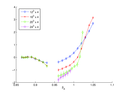
Figure 9: Free energy $aN_{\tau}F_{V}$ along the $\lambda=0.8$ paths of Fig. 1.

The data points start right on top of the bulk transition and go on up to slightly above the finite temperature deconfinement transition. The behaviour up to the bulk transition is in agreement with the ’t Hooft vortex argument for confinement: if vortices behave ”chaotically” ($F=0$) then the theory confines (phase I), while as deconfinement occurs $F\sim\tilde{\sigma}N_{s}^{2}$. As explained above, we cannot actually go too deeply into the deconfined phase, so we cannot check if for $\beta_{A}\gg\beta_{A}^{c}$ the data are consistent with $O(N_{s}^{2})$ plateaus or if they saturate at some value in the thermodynamic limit, i.e. if a dual string tension $\tilde{\sigma}$ can indeed be measured. To this purpose, assuming that the estimate in Eq. (10) still works at higher $\beta_{A}$, even taking into account that for higher volumes the asymptotic behaviour should kick in earlier, we would need to simulate around 50 parallel ensembles for each volume, again for a statistics of at least $O(10^{5})$ per configuration in each ensemble. For volumes with $N_{s}\geq 20$, for which finite size effects start to be reasonably small, this goes beyond the computational power at our disposal, although it should be manageable with a medium sized PC cluster. A reliable estimate of $\tilde{\sigma}$ would be of extreme interest in light of the behaviour we find for $F$ in the confined phase of phase II, already reported in Ref. Burgio et al. (2006a). Vortex production is there clearly enhanced compared to phase I and the free energy stays negative up to the deconfinement transition, where it rises to positive values.

Fig. 10 shows the free energy in a low $\beta_{A}$ confining region well below the finite temperature transition. The negative plateau values away from the bulk transition at $\lambda_{c}(\beta_{A})$ are consistent with what is observed in Fig. 9 and with a vanishing free energy in the limit $T\to 0$ Kovacs and Tomboulis (2000), since its value rises again for decreasing $\beta_{A}$ after reaching a minimum around $\beta_{A}=0.65$. Larger volumes and a better extrapolation would be of course needed to confirm this result.

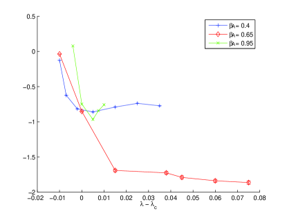
Figure 10: Free energy $aN_{\tau}F_{V}$ for varying $\lambda-\lambda_{c}$ at fixed $\beta_{A}$ and lattice size $16^{3}\times 4$ (see Table 6).

As for the higher twists, although being proper only to the toroidal topology they also show a surprising and interesting behaviour. Namely, we do not observe a free energy proportional to the difference in topological index as one would have expected if the twist observables $z_{i,4}$ were independent. We indeed observe a strong correlation among the twist in the different planes, indicating a non trivial interaction among vortices; as a result in the confined phase, although the population of the $\pm 1$ sectors for the single $z_{i,4}$ are comparable, the distribution of the $\nu_{k}$ is such to follow the hierarchy $\nu_{2}/3\gtrsim\nu_{3}\gtrsim\nu_{1}/3\gg\nu_{0}$. E.g. for $N_{s}=24$, $\lambda=0.8$ and $\beta_{A}=0.96$ we find $\nu_{0}=0.020(1)$, $\nu_{1}=0.35(5)$, $\nu_{2}=0.48(4)$ and $\nu_{3}=0.15(2)$. Such hierarchy is quite stable with the volume for $N_{s}\geq 16$. Taking into account that when calculating $F$ $\nu_{1}$ and $\nu_{2}$ need to be rescaled by a factor three to be compared with sectors $\nu_{0}$ and $\nu_{3}$, errors are still to high within the statistics at our disposal to allow a reliable measure of the free energy for the tunnelling other than from/to the 0 sector. Approaching and crossing the deconfinement transition the situation changes. The trivial sector starts to dominate the partition function and the free energy to tunnel from one sector to another becomes indeed proportional to the difference in their topological index. Being the higher sectors however exponentially suppressed in the deconfined phase their sampling requires longer and longer runs as $\beta_{A}$ increases; the sampling of sectors with topological index higher than one will become in practice eventually unfeasible.

IV.3 $C^{*}$ boundary conditions, monopoles and $F$

An interesting alternative check of our surprising negative value for $F$ is the evaluation of the vortex free energy for the modified action $S^{M}$ needed to define the Pisa disorder parameter in Sec. IV.1. As already discussed in Sec. II, $C^{*}$ boundary conditions in the Euclidean time direction $U(x+aN_{\tau}\hat{t})=U^{*}(x)$ pose no conceptual problem in our adjoint formulation. Any set of twist matrices $\{\Omega\}$ in the fundamental representation once projected onto the adjoint representation become gauge equivalent to periodic boundary conditions de Forcrand and Jahn (2003). Given that any set $\{\Omega\}$ is gauge equivalent to the quaternion basis $\{\mathbb{I}_{2},i\vec{\sigma}\}$ and since $C^{*}$ boundary conditions can be represented through the action of $\Omega_{2}=i\sigma_{2}$, $U^{*}(x)=\Omega_{2}U(x)\Omega^{\dagger}_{2}$, imposing them makes no difference in the dynamics of twist sectors: the configurations that can be assigned to a given twist will simply be relabeled with respect to standard boundary conditions. In other words the corresponding combination of adjoint twist matrices, which would satisfy a given twist algebra when lifted to $SU(2)$, get reshuffled by the presence of $i\sigma_{2}$. A simple listing of combinations shows however that the number of states leading to the assignment of topological sectors $z=0,\ldots,3$ remains the same.

$C^{*}$ boundary conditions alone therefore should not affect the value of $F$ for $S^{M}$. There is however the bosonic field giving rise to the abelian monopole through its non-trivial transformation property at the boundary $\pi_{2}(SU(2)/U(1))=\pi_{1}(U(1))=\mathbb{Z}$ Di Giacomo and Paffuti (1997); Fröhlich and Marchetti (2001); its rôle is far deeper and more interesting. For a Lie gauge group $G$ with center ${{K}}$ and a maximal Cartan subalgebra ${{C}}$ it is well known that the abelian monopoles classified by $\pi_{2}(G/{{C}})=\pi_{1}({{C}})$ will carry center magnetic charges classified by $\pi_{1}(G/{{K}})$ Lubkin (1963); only the ones belonging to the kernel of $\pi_{1}({{C}})\to\pi_{1}(G/{{K}})$ will be non singular Lubkin (1963); Coleman (1982). For $SU(N)$ this simply means that the $N-1$ abelian monopoles classified by $\mathbb{Z}^{N-1}$ will also correspond to $N-1$ $\mathbb{Z}_{N}$ monopoles; their corresponding Dirac strings (sheets in a 3+1 Euclidean formulation) will be in general open $\mathbb{Z}_{N}$ vortices.

In the simple case of $SU(2)$ the assignment is quite easy: to an abelian charge $n\in\mathbb{Z}$ will correspond a $\mathbb{Z}_{2}$ monopole of charge ${\rm mod}_{2}(n)\in\mathbb{Z}_{2}$. Only monopoles of charge $n=2k$ carry no singularity along their world line; odd charged monopoles are singular in every gauge. The world line of the latter saturates an open $\mathbb{Z}_{2}$ vortex, while only the former are compatible with closed (or no) vortex sheets Fröhlich and Marchetti (2001). Our situation is however slightly different: $C^{*}$ boundary conditions take care of magnetic charge conservation by making the unit charge abelian monopole being put by hand into the system his own antimonopole; the Dirac sheet of the $\mathbb{Z}_{2}$ vortex starting on the monopole ends on itself. Such vortex is therefore spatially closed but cut through by a singularity along the world line of the abelian monopole. Moreover such “cut” cannot be gauged around; the vortex is “pinned” down along one line by the singularity. This should however not be detectable by $F$: the creation of a further vortex will bring the system in a state which for our purpose can aways be assimilated to either a 2- or 0-twist sector. This will make no difference below the bulk transition, where the partition function is dominated by open vortices anyway and all twist sectors are equivalent: $F$ should still vanish there. In the deconfined phase $T>T_{c}$ the cost to create a further vortex should still scale like $N_{s}^{2}$, no matter what the background is, so that $F$ should become again large and positive. Only in the confined phase of phase II, if the system prefers the vortex background, there should be a difference between $S$ and $S^{M}$: if in the former $F$ is negative it should become positive in the latter. Fig. 11 shows this to be the case:

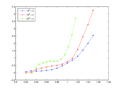
Figure 11: $aN_{\tau}F_{V}$ for $S^{M}$ along the $\lambda=0.8$ paths of Fig. 1.

in the (singular) vortex background of $S^{M}$ the system prefers to make the creation of one further vortex more expensive. Notice that the position of the bulk is slightly different for $S$ and $S^{M}$, e.g. at $\lambda=0.8$ it shifts from $\beta_{A}\simeq 0.89-0.90$ to $\beta_{A}\simeq 0.92-0.93$; starting our PT ensemble right on top of it we are able to span the range of couplings in one single run, reaching however the limits of our acceptance rate criterion for $N_{s}=20$. Why $F$ turns out roughly to be minus the half of what it was for $S$ is not obvious. It might be related to the non-standard character of the $S^{M}$ vortex background or to the effective superposition of 0- and 2-twist sectors. In light of a recent proposal Rajantie (2006) such observable could also be linked to the direct evaluation of the monopole mass.

The previous discussion offers also an elegant explanation both to the sensitivity of $\rho$ to the bulk transition and to its non-vanishing in the low $\beta_{A}$ limit of phase II observed in Barresi et al. (2004d); Barresi and Burgio (2006) and already discussed in Sec. IV.1. Action $S$, consistently with what is expected in the continuum limit, completely suppresses the presence of $\mathbb{Z}_{2}$ monopoles, allowing only topological, i.e. closed, vortices. The construction of $\rho$ we have adopted, following Di Giacomo and Paffuti (1997); Barresi et al. (2004d), uses a unit charged abelian monopole, which as discussed above introduces a singularity exactly through the presence of a $\mathbb{Z}_{2}$ monopole. The physical states described by $S$ can therefore never be equivalent to those of $S^{M}$ and hence the discrepancy. This was already “predicted” in Ref. Fröhlich and Marchetti (2001), where an alternative construction using even charged monopoles was proposed as the only one fully consistent with the continuum pure Yang-Mills action. Singular gauge configurations will not be allowed there and only genuinely closed vortices will exist. Such modified construction should therefore be the obvious choice for adjoint actions and its feasibility might be worth to explore. The discrepancy in $\rho$ observed here cannot be detected through actions transforming with the fundamental representation: although they should disappear in the continuum limit, $\mathbb{Z}_{2}$ monopoles are still present both with and without monopole background in the range of parameters commonly used in simulations, while the topological structure of vortices is anyway blurred by the fixed boundary conditions.

V Electric flux and vanishing of $F$

A few comments are in order to clarify some properties of $F$ discussed in the literature which could seem to be in conflict with our result. In Ref. ’t Hooft (1979) an exact duality relation between electric and magnetic fluxes implying the vanishing of $F$ was proved under two main assumptions: first one must be able to define a set of regularized operators in the fundamental representation; second the limit $T\to 0$ has to be taken after the finite temperature compactification of the time direction. As for the latter, we actually agree with $F=-T\Delta S\to 0$ as $T\to 0$, which is almost obvious in our formulation. The former condition has more far reaching consequences. It was extended to finite temperature and is indeed the key point of the derivations of many interesting dynamical relations in Yang-Mills theories, mostly using reflection positivity for the fundamental Wilson action on the lattice Tomboulis and Yaffe (1985). In an adjoint discretization however observables like the fundamental Polyakov loop, the fundamental trace of the electric flux free energy etc. needed to prove such relations are all undefined. Formally their expectation values and all their correlators vanish identically.

This can be better understood within the Hamiltonian formulation of lattice Yang-Mills theories, adapting the exact construction of the $SU(2)$ Hilbert space given in Ref. Burgio et al. (2000). Since the irreducible representations of $SO(3)$ are simply the integer representations of $SU(2)$, the Hilbert space of $SO(3)$-invariant states in each twist sector is given by the subset of the $SU(2)$ states described in Ref. Burgio et al. (2000) (with corresponding t.b.c.) with all links and intertwiners labelled by integer spins only. Since topological sectors are automatically accounted for in $SO(3)$ with p.b.c. we have $\mathcal{H}_{SO(3)}=\bigoplus_{i}\mathcal{H}^{i}_{SO(3)}$, $~{}i~{}$ being the winding number corresponding to the twist sectors, with $\mathcal{H}^{i}_{SO(3)}\subset\mathcal{H}^{i}_{SU(2)}$ the fixed twist spaces mentioned above. It is now straightforward to see how fundamental operators annihilate the Hilbert space of $SO(3)$-invariant states. Let us illustrate this by an example. Take a fundamental Wilson loop, winding or not around the boundaries: on the $SU(2)$ Hilbert space such operator can be represented as a closed string of spin 1/2 located on the corresponding links; as proven in Ref. Burgio et al. (2000) its action on a generic $SU(2)$ state will generate states where the representations labelling the links and intertwiners of interest are simply composed with the 1/2 representation via the common spin composition rules. Since a state in the $SO(3)$-invariant subspace defined above will only carry integer spins, its composition with our operator will generate states which will necessarily carry semi-integer representations on the links of interest, i.e. it will not belong to $\mathcal{H}_{SO(3)}$ anymore. Generalizing, the action of a fundamental operator $\mathcal{F}$ on a state $\psi=\sum_{i}\lambda_{i}\psi_{i}$, $~{}\psi_{i}\in\mathcal{H}^{i}_{SO(3)}$ will generate states living in the orthogonal complements of $\mathcal{H}^{i}_{SO(3)}$ in $\mathcal{H}^{i}_{SU(2)}$, $\mathcal{F}\psi_{i}\in\mathcal{H}^{i,\bot}_{SO(3)}$ with

$$\mathcal{H}^{i}_{SU(2)}=\mathcal{H}^{i}_{SO(3)}\bigoplus\mathcal{H}^{i,\bot}_{SO(3)}\,.$$ (18)

When the dynamics can be described by a Hamiltonian $H=E_{c}+V$ transforming under the adjoint representation, as it is the case for Eq. (1), it is legitimate to restrict the whole treatment to $\mathcal{H}_{SO(3)}$. Then obviously $\mathcal{F}\mathcal{H}_{SO(3)}\equiv 0$, which is by definition the only state in the intersection $~{}\mathcal{H}^{i}_{SO(3)}\bigcap\mathcal{H}^{i,\bot}_{SO(3)}$.

A trivial consequence of the above arguments is that with an adjoint action reflection positivity constraints can only be invoked for adjoint observables, ensuring e.g. that adjoint Polyakov loop correlators will be positive definite; constraints derived from fundamental operators will be invalid. This concerns e.g. the reflection positivity constraints among fundamental Wilson loops, static quark potential, electric flux free energy and vortex free energy (see e.g. Appendix I in Ref. Tomboulis and Yaffe (1985)). In particular this latter constraint is interesting since it could seem to contradict our result for $F$. Such relation between the Fourier transform of the vortex free energy and the electric flux free energy, essential to derive the vanishing of $F$ in the confined phase, is ill defined in an adjoint theory, since it needs the action of a fundamental maximal Wilson loop winding around the space boundary to be established, as in Eq. (4.6) of ’t Hooft (1979). With an adjoint weight in the partition function Eqs. (4.9) and (4.10) of the above reference become identically zero. Therefore the operator there given in Eq. (5.2), although still well defined, cannot be related to the projector onto a state of fixed electric flux. Also the alternative definition given in Ref. de Forcrand and von Smekal (2002) through fundamental Polyakov loops $~{}L_{F}~{}$ modified via a twist eater at the time boundary is only valid in a fundamental theory (with twisted boundary conditions). In an adjoint theory the first line of their Eq. (15) cannot be inverted. Alternatively, correlators of $L_{F}$ will in general vanish identically giving no useful bound on their sign via reflection positivity for the only potentially non-vanishing case of maximal displacement. There is therefore no guarantee that the right hand side of their Eq. (16) will be positive, i.e. that it can indeed be interpreted as the exponential of a free energy.

An electric flux operator can of course be defined also in our adjoint model: it will simply be given by an adjoint maximal Wilson loop winding around the space boundary. Such operator cannot however be related to the vortex free energy as defined in Eq. (4).

VI Conclusions

In this paper we have studied on the lattice at finite temperature a pure $SO(3)$ gauge theory, which transforms under the actual gauge symmetry group of pure $SU(2)$ Yang-Mills in the continuum. Extending the analysis in Ref. Burgio et al. (2006a) we have employed the Pisa disorder operator for monopole condensation to establish the properties of the theory within the weak coupling phase II, which allows a well defined continuum limit, finding confined and deconfined phases separated by a transition of presumably second order consistent with the universality class of Ising 3-d.

The vortex free energy $F$ is however found not to vanish at $T\neq 0$ in the confined phase of $SO(3)$. As discussed above, standard arguments for its vanishing up to $T_{c}$ cannot be applied when working with an adjoint action, so that our result is in itself not contradictory. Moreover, the vanishing of $~{}F~{}$ in the confined phase is in general just a sufficient condition for confinement. The full adjoint theory discussed here possesses neither center symmetry nor well defined fundamental observables. Only adjoint observables make any sense, a fundamental string tension being impossible to calculate. There seems therefore no compelling physical reason for the ’t Hooft vortex free energy to vanish for $T\neq 0$, since this would be linked to an area law behaviour of fundamental Wilson loops, i.e. to the existence of a fundamental string tension, which however loses its meaning as soon as the specific properties of semi-integer discretizations are lifted. Indeed, it would be surprising to establish the existence of an order parameter for the breaking of a symmetry the theory does not possess Holland et al. (2003). This however does not in our opinion violate universality, since such properties are not essential to describe the dynamics of continuum pure Yang-Mills theories. Only physical properties like deconfinement temperature and universality class or the glueball spectrum are preserved independently of the discretization used. Only those should therefore be addressed in trying to establish a topological mechanism of confinement valid both in pure Yang-Mills theories and in full QCD. If no symmetry breaking and therefore no order parameter is available the properties of the phase transition can still be established through the specific heat or other thermodynamic observables Datta and Gavai (2000, 1999).

The non-vanishing of $F$ implies that the dual string tension cannot serve as an order parameter for the adjoint theory. For this purpose it would need to vanish exponentially in the thermodynamic limit in the confined phase, while our simulations indicate that it will vanish at most as $O(N_{s}^{-2})$. Our results show therefore that between the monopole condensation parameter and the ’t Hooft vortex free energy (i.e. a dual string tension) only the former seems to retain all its order-parameter character independently of the discretization used, at least once rescaled to assume a constant value in the confined phase. This is a simple consequence of its property to vanish exponentially above the critical temperature, as e.g. the magnetization for a ferromagnet. The rescaling should anyway become unnecessary if one adopts the alternative prescriptions given in Fröhlich and Marchetti (2001). Monopole condensation can therefore play the rôle of an order parameter both for the $SU(2)$ invariant quenched theory, possessing center symmetry but no vortex topological sectors, and for the $SO(3)$ invariant pure Yang-Mills theory, where center symmetry is absent. Vortex topology does not provide there a suitable order parameter.

Why the 0-twist sector gets strongly suppressed in the confined phase causing vortex free energy to take a negative value, i.e. why the Yang-Mills action finds it energetically favorable to create at least one vortex, and why twist observables in different directions hint at a non trivial interaction pattern among vortices are questions which need to be answered and that we will try to address in the near future.

References

- McLerran and Svetitsky (1981) L. D. McLerran and B. Svetitsky, Phys. Lett. B98, 195 (1981).
- Kuti et al. (1981) J. Kuti, J. Polonyi, and K. Szlachanyi, Phys. Lett. B98, 199 (1981).
- Polyakov (1978) A. M. Polyakov, Phys. Lett. B72, 477 (1978).
- Susskind (1979) L. Susskind, Phys. Rev. D20, 2610 (1979).
- Smilga (1994) A. V. Smilga, Ann. Phys. 234, 1 (1994).
- Svetitsky and Yaffe (1982) B. Svetitsky and L. G. Yaffe, Nucl. Phys. B210, 423 (1982).
- ’t Hooft (1978) G. ’t Hooft, Nucl. Phys. B138, 1 (1978).
- ’t Hooft (1979) G. ’t Hooft, Nucl. Phys. B153, 141 (1979).
- de Forcrand and Jahn (2003) P. de Forcrand and O. Jahn, Nucl. Phys. B651, 125 (2003), eprint hep-lat/0211004.
- Bhanot and Creutz (1981) G. Bhanot and M. Creutz, Phys. Rev. D24, 3212 (1981).
- Greensite and Lautrup (1981) J. Greensite and B. Lautrup, Phys. Rev. Lett. 47, 9 (1981).
- Halliday and Schwimmer (1981a) I. G. Halliday and A. Schwimmer, Phys. Lett. B101, 327 (1981a).
- Halliday and Schwimmer (1981b) I. G. Halliday and A. Schwimmer, Phys. Lett. B102, 337 (1981b).
- Cheluvaraja and Sharathchandra (1996) S. Cheluvaraja and H. S. Sharathchandra (1996), eprint hep-lat/9611001.
- Datta and Gavai (1998) S. Datta and R. V. Gavai, Phys. Rev. D57, 6618 (1998), eprint hep-lat/9708026.
- Datta and Gavai (2000) S. Datta and R. V. Gavai, Nucl. Phys. Proc. Suppl. 83, 366 (2000), eprint hep-lat/9908040.
- Datta and Gavai (1999) S. Datta and R. V. Gavai, Phys. Rev. D60, 034505 (1999), eprint [http://arXiv.org/abs]hep-lat/9901006.
- Mack and Petkova (1982) G. Mack and V. B. Petkova, Zeit. Phys. C12, 177 (1982).
- Tomboulis (1981) E. Tomboulis, Phys. Rev. D23, 2371 (1981).
- Kovacs and Tomboulis (1998) T. G. Kovacs and E. T. Tomboulis, Phys. Rev. D57, 4054 (1998), eprint hep-lat/9711009.
- Alexandru and Haymaker (2000) A. Alexandru and R. W. Haymaker, Phys. Rev. D62, 074509 (2000), eprint hep-lat/0002031.
- Swendsen and Wang (1987) R. H. Swendsen and J.-S. Wang, Phys. Rev. Lett. 58, 86 (1987).
- Berg and Neuhaus (1991) B. A. Berg and T. Neuhaus, Phys. Lett. B267, 249 (1991).
- Barresi et al. (2002) A. Barresi, G. Burgio, and M. Müller-Preussker, Nucl. Phys. Proc. Suppl. 106, 495 (2002), eprint hep-lat/0110139.
- Barresi et al. (2003) A. Barresi, G. Burgio, and M. Müller-Preussker, Nucl. Phys. Proc. Suppl. 119, 571 (2003), eprint hep-lat/0209011.
- Barresi and Burgio (2006) A. Barresi and G. Burgio, to appear on Eur. Phys. J. C (2006), eprint hep-lat/0608008.
- Michael (1985) C. Michael, Nucl. Phys. B259, 58 (1985).
- Barresi et al. (2004a) A. Barresi, G. Burgio, and M. Müller-Preussker, Phys. Rev. D69, 094503 (2004a), eprint hep-lat/0309010.
- Barresi et al. (2004b) A. Barresi, G. Burgio, and M. Müller-Preussker, Nucl. Phys. Proc. Suppl. 129, 695 (2004b).
- Barresi et al. (2004c) A. Barresi, G. Burgio, and M. Müller-Preussker, Color confinement and hadrons in quantum chromodynamics Wako 2003, 82 (2004c), eprint hep-lat/0312001.
- Barresi et al. (2004d) A. Barresi, G. Burgio, M. D’Elia, and M. Müller-Preussker, Phys. Lett. B599, 278 (2004d), eprint hep-lat/0405004.
- de Forcrand and von Smekal (2002) P. de Forcrand and L. von Smekal, Phys. Rev. D66, 011504(R) (2002), eprint hep-lat/0107018.
- Burgio et al. (2006a) G. Burgio, M. Fuhrmann, W. Kerler, and M. Müller-Preussker, Phys. Rev. D74, 071502(R) (2006a), eprint hep-th/0608075.
- Burgio et al. (2006b) G. Burgio, M. Fuhrmann, W. Kerler, and M. Müller-Preussker, PoS LAT2005, 288 (2006b), eprint hep-lat/0607034.
- Di Giacomo and Paffuti (1997) A. Di Giacomo and G. Paffuti, Phys. Rev. D56, 6816 (1997), eprint hep-lat/9707003.
- Di Giacomo et al. (2000a) A. Di Giacomo, B. Lucini, L. Montesi, and G. Paffuti, Phys. Rev. D61, 034503 (2000a), eprint hep-lat/9906024.
- Di Giacomo et al. (2000b) A. Di Giacomo, B. Lucini, L. Montesi, and G. Paffuti, Phys. Rev. D61, 034504 (2000b), eprint hep-lat/9906025.
- Carmona et al. (2001) J. M. Carmona, M. D’Elia, A. Di Giacomo, B. Lucini, and G. Paffuti, Phys. Rev. D64, 114507 (2001), eprint hep-lat/0103005.
- Fröhlich and Marchetti (2001) J. Fröhlich and P. A. Marchetti, Phys. Rev. D64, 014505 (2001), eprint hep-th/0011246.
- Marinari and Parisi (1992) E. Marinari and G. Parisi, Europhys. Lett. 19, 451 (1992), eprint hep-lat/9205018.
- Kerler and Weber (1993) W. Kerler and A. Weber, Phys. Rev. B47, 11563 (1993), eprint hep-lat/9306022.
- Kerler and Rehberg (1994) W. Kerler and P. Rehberg, Phys. Rev. E50, 4220 (1994).
- Kerler et al. (1994) W. Kerler, C. Rebbi, and A. Weber, Phys. Rev. D50, 6984 (1994), eprint hep-lat/9403025.
- Kerler et al. (1995) W. Kerler, C. Rebbi, and A. Weber, Nucl. Phys. B450, 452 (1995), eprint hep-lat/9503021.
- Boyd (1996) G. Boyd (1996), eprint hep-lat/9701009.
- Hukushima and Nemoto (1995) K. Hukushima and K. Nemoto (1995), eprint cond-mat/9512035.
- Marinari (1996) E. Marinari (1996), eprint cond-mat/9612010.
- Boyd (1998) G. Boyd, Nucl. Phys. Proc. Suppl. 60A, 341 (1998), eprint hep-lat/9712012.
- Joo et al. (1999) B. Joo et al. (UKQCD), Phys. Rev. D59, 114501 (1999), eprint hep-lat/9810032.
- Ilgenfritz et al. (2000a) E.-M. Ilgenfritz, W. Kerler, and H. Stüben, Nucl. Phys. Proc. Suppl. 83, 831 (2000a), eprint hep-lat/9908022.
- Ilgenfritz et al. (2000b) E. M. Ilgenfritz, W. Kerler, M. Müller-Preussker, and H. Stüben (2000b), eprint hep-lat/0007039.
- Ilgenfritz et al. (2002) E.-M. Ilgenfritz, W. Kerler, M. Müller-Preussker, and H. Stüben, Phys. Rev. D65, 094506 (2002), eprint hep-lat/0111038.
- Priestley (1989) M. B. Priestley, Spectral analysis and time series, Academic Press, London (1989).
- Madras and Sokal (1988) N. Madras and A. D. Sokal, J. Statist. Phys. 50, 109 (1988).
- Wolff (1989) U. Wolff, Phys. Lett. B228, 379 (1989).
- Kerler (1993a) W. Kerler, Phys. Rev. D47, R1285 (1993a).
- Kerler (1993b) W. Kerler, Phys. Rev. D48, 902 (1993b), eprint hep-lat/9306021.
- Brandt (1976) S. Brandt, Statistical and computational methods in data analysis, North-Holland, Amsterdam (1976).
- Kovacs and Tomboulis (2000) T. G. Kovacs and E. T. Tomboulis, Phys. Rev. Lett. 85, 704 (2000), eprint hep-lat/0002004.
- Lubkin (1963) E. Lubkin, Ann. Phys. 23/2, 233 (1963).
- Coleman (1982) S. R. Coleman (1982), lectures given at Int. Sch. of Subnuclear Phys., Erice, Italy, Jul 31-Aug 11, 1981.
- Rajantie (2006) A. Rajantie, JHEP 01, 088 (2006), eprint hep-lat/0512006.
- Tomboulis and Yaffe (1985) E. T. Tomboulis and L. Yaffe, Commun. Math. Phys. 100, 313 (1985).
- Burgio et al. (2000) G. Burgio, R. De Pietri, H. A. Morales-Tecotl, L. F. Urrutia, and J. D. Vergara, Nucl. Phys. B566, 547 (2000), eprint hep-lat/9906036.
- Holland et al. (2003) K. Holland, P. Minkowski, M. Pepe, and U. J. Wiese, Nucl. Phys. B668, 207 (2003), eprint hep-lat/0302023.