Radiative $\phi$$-$meson decays and $\eta$-$\eta^{\prime}$ mixing: a QCD sum rule analysis

Abstract:

The radiative transitions $\phi\to\eta\gamma$ and $\phi\to\eta^{\prime}\gamma$ are analysed using QCD sum-rules. At leading order in perturbative QCD, we obtain the results: ${\cal B}(\phi\to\eta\gamma)=(1.15\pm 0.2)~{}10^{-2}$ and ${\cal B}(\phi\to\eta^{\prime}\gamma)=(1.18\pm 0.4)~{}10^{-4}$, in very good agreement with existing experimental data. The related issue of $\eta-\eta^{\prime}$ mixing is discussed and we give predictions for the $\eta$ and $\eta^{\prime}$ decay constants in the framework of a mixing scheme in the quark-flavour basis.

1 Introduction

Radiative $\phi$ meson decays represent an important source of information on low-energy hadron physics, shedding light, for example, on the structure and properties of low-mass resonances, such as the $f_{0}(980)$. In particular, radiative $\phi$ decays to $\eta$ and $\eta^{\prime}$ can provide insights into the long standing problem of $\eta-\eta^{\prime}$ mixing and probe the strange quark content of the light pseudoscalars [1, 2]. Radiative $\phi$ decays, not only raise interesting theoretical issues, but are an important focus of the data-taking by the KLOE experiment at the DA$\Phi$NE $\phi$-factory [3], where a large sample of $\phi$ decays will be collected, dramatically improving the experimental information already obtained by the VEPP$-$2M groups at Novosibirsk [4].

This paper is devoted to the analysis of the radiative $\phi\to\eta\gamma$ and $\phi\to\eta^{\prime}\gamma$ transitions. In contrast to the light vector meson case, where the $\omega$ and $\phi$ are recognised as almost ideally mixed states with quark content of well defined flavour, $\eta-\eta^{\prime}$ mixing is still a much debated subject. The once conventional description was to adopt a single mixing angle in the octet-singlet flavour basis. Various attempts to estimate such an angle lead to results ranging from $-10^{0}$ to $-20^{0}$ [5]. More recently, Leutwyler et al. [6, 7] have shown that a consistent treatment of the $\eta-\eta^{\prime}$ system requires the introduction of two mixing angles with a consequent redefinition of the particle decay constants. An equivalent description, as explained in more detail below, is obtained if the mixing basis is chosen to be the quark-flavour basis instead of the octet-singlet one [8]. In such a scheme, it has been shown that a description in terms of a single mixing angle is quite reliable leading to predictions satisfying constraints from Chiral Perturbation Theory [6].

In this context a central role is played by the $U(1)_{A}$ anomaly. Since the flavour-singlet axial vector current is not conserved due to this anomaly, the $\eta^{\prime}$ meson cannot be identified as the ninth Goldstone boson. This crudely explains the fact that the $\eta^{\prime}$ is much heavier than the other members of the pseudoscalar nonet. By combining chiral symmetry with the concepts of the large $N_{c}$ limit of QCD, Leutwyler[9] has extended Chiral Perturbation Theory from an expansion in the light quark masses and momenta to encompass powers of ${1/N_{c}}$. Then in the limit $N_{c}\to\infty$, the $U(1)_{A}$ anomaly vanishes and the $\eta^{\prime}$ can formally be identified with the ninth Goldstone boson. In order to make the framework more predictive and closer to reality, correction terms are added to the effective Lagrangian of the theory, expressing the deviation from the chiral limit for the decay constants and the masses of the light mesons. A Wess-Zumino-Witten (WZW) term describing the anomalous coupling to photons must also be added. Radiative $\phi$ decays provide additional information on the strength of this WZW term.

In the following we analyse $\phi$ radiative decays using QCD sum-rules [10] at leading order in perturbative QCD. These sum-rules are widely recognised as a reliable technique for including the effects of non-perturbative QCD. In section 2 we survey possible $\eta-\eta^{\prime}$ mixing schemes, with particular emphasis on the flavour basis mixing scheme developed by Feldmann et al. [8]. We give the relation between the parameters characterising such a scheme and those in the octet-singlet basis. In section 3, as a preliminary to our analysis of $\phi$ radiative decays, we compute the coupling of the strange pseudoscalar current both to the $\eta$ and $\eta^{\prime}$ mesons using two-point QCD sum-rules. These provide key inputs into the three-point QCD sum-rule developed to estimate the decay widths $\Gamma(\phi\to\eta\gamma)$ and $\Gamma(\phi\to\eta^{\prime}\gamma)$, in section 4. The possible effect of ${\cal O}(\alpha_{s})$ corrections is discussed at the end of this section.

Though we often refer to the problem of mixing and we actually work with interpolating currents defined in the quark flavour basis, our results do not depend on any specific mixing scheme and so provide a genuinely mixing scheme independent set of QCD predictions. If then a particular flavour mixing scheme is adopted, our results can be translated into a prediction for one of the mixing angles. In section 5 we again use two-point QCD sum-rules to compute the coupling of $\eta$ and $\eta^{\prime}$ to the strange and non-strange axial currents, identifying the results with the decay constants in the flavour basis mixing scheme. The results again allow us to estimate the mixing parameters in such a scheme. The results in sections 3 and 5 can be exploited to obtain an estimate of the contribution of the anomaly to the couplings computed in section 3. In section 6 we draw our conclusions.

2 On $\eta-\eta^{\prime}$ Mixing

Let us first recall the usual parametrization of $\eta-\eta^{\prime}$ mixing in the octet-singlet basis. We define current-particle matrix elements as

$$<0|J_{5\mu}^{i}|P(p)>=i~{}f_{P}^{i}p_{\mu}\;\;\;(i=8,0;~{}~{}~{}P=\eta,\eta^{\prime})\;,$$ (1)

with $J_{5\mu}^{8}$ the $SU(3)_{F}$ octet axial vector current:

$$J_{5\mu}^{8}={1\over\sqrt{6}}\left({\overline{u}}\gamma_{\mu}\gamma_{5}u+{\overline{d}}\gamma_{\mu}\gamma_{5}d-2{\overline{s}}\gamma_{\mu}\gamma_{5}s\right)$$ (2)

and $J_{5\mu}^{0}$ the singlet current:

$$J_{5\mu}^{0}={1\over\sqrt{3}}\left({\overline{u}}\gamma_{\mu}\gamma_{5}u+{\overline{d}}\gamma_{\mu}\gamma_{5}d+{\overline{s}}\gamma_{\mu}\gamma_{5}s\right)\;.$$ (3)

As already mentioned, two mixing angles, $\theta_{8}$ and $\theta_{0}$, are required [9] in order to treat mixing consistently. Accordingly, the couplings in (1) can be defined as follows:

$$f_{\eta}^{8}=f_{8}~{}\cos\theta_{8} \hskip 28.45274ptf_{\eta}^{0}=-f_{0}~{}\sin\theta_{0}$$

$$f_{\eta^{\prime}}^{8}=f_{8}~{}\sin\theta_{8} \hskip 28.45274ptf_{\eta^{\prime}}^{0}=f_{0}~{}\cos\theta_{0}\;.$$ (4)

Alternatively we can consider two independent axial vector currents with distinct quark flavour:

$$J_{5\mu}^{q} = {1\over\sqrt{2}}({\overline{u}}\gamma_{\mu}\gamma_{5}u+{\overline{d}}\gamma_{\mu}\gamma_{5}d)$$

$$J_{5\mu}^{s} = {\overline{s}}\gamma_{\mu}\gamma_{5}s\;.$$ (5)

The couplings of the $\eta$ and $\eta^{\prime}$ mesons to the currents (5) can be defined analogously to (1). The decay constants are written according to the following mixing pattern:

$$f_{\eta}^{q}=f_{q}~{}\cos\phi_{q} \hskip 28.45274ptf_{\eta}^{s}=-f_{s}~{}\sin\phi_{s}$$

$$f_{\eta^{\prime}}^{q}=f_{q}~{}\sin\phi_{q} \hskip 28.45274ptf_{\eta^{\prime}}^{s}=f_{s}~{}\cos\phi_{s}\;\;\;\;.$$ (6)

Though there are, of course, two angles in each basis, Feldmann [8] has shown that the mixing is specified quite accurately in terms of a single mixing angle, i.e. $\phi_{q}=\phi_{s}=\phi$, since $|\phi_{s}-\phi_{q}|/(\phi_{s}+\phi_{q})\ll 1$, resulting in a much simpler framework. In this approximation, the states follow the same mixing pattern as the decay constants:

$$|\eta> = \cos\phi~{}|\eta_{q}>-\sin\phi~{}|\eta_{s}>$$

$$|\eta^{\prime}> = \sin\phi~{}|\eta_{q}>+\cos\phi~{}|\eta_{s}>$$ (7)

where $|\eta_{q}>$ and $|\eta_{s}>$ have a quark content defined by ideal mixing. We will refer to this simply as mixing in the quark-flavour basis, in order to distinguish it from the previous one, which will be referred to as mixing in the octet-singlet basis. It is straightforward to obtain the relations between the parameters in the two mixing schemes:

$$\tan~{}\theta_{8}={f_{q}\,\sin\phi_{q}-\sqrt{2}f_{s}\,\cos\phi_{s}\over f_{q}\,\cos\phi_{q}+\sqrt{2}f_{s}\,\sin\phi_{s}}\;\;\;,\;\;\;\;\tan~{}\theta_{0}={f_{s}\,\sin\phi_{s}-\sqrt{2}f_{q}\,\cos\phi_{q}\over f_{s}\,\cos\phi_{s}+\sqrt{2}f_{q}\,\sin\phi_{q}}$$ (8)

which become, for $\phi_{q}=\phi_{s}=\phi$ [8]:

$$\theta_{8}=\phi-\arctan\left({\sqrt{2}f_{s}\over f_{q}}\right)\hskip 28.45274pt\theta_{0}=\phi-\arctan\left({\sqrt{2}f_{q}\over f_{s}}\right)\;.$$ (9)

Moreover:

$$f_{8}^{\,2} = {1\over 3}f_{q}^{\,2}+{2\over 3}f_{s}^{\,2}+{2\sqrt{2}\over 3}f_{q}f_{s}\sin(\phi_{s}-\phi_{q})$$

$$f_{0}^{\,2} = {2\over 3}f_{q}^{\,2}+{1\over 3}f_{s}^{\,2}-{2\sqrt{2}\over 3}f_{q}f_{s}\sin(\phi_{s}-\phi_{q})\;\;.$$ (10)

In the following sections we derive the ingredients necessary for the description of the radiative $\phi\to\eta\gamma$ and $\phi\to\eta^{\prime}\gamma$ decays, without assuming any specific mixing framework. Then, in section 5, we will evaluate the couplings of the $\eta$ and $\eta^{\prime}$ to the axial vector current and estimate the parameters appearing in (6), obtaining a prediction for $\phi_{q}$, $\phi_{s}$. At the end, we shall comment on the accuracy of the approximation $\phi_{q}=\phi_{s}$.

3 Two-point function for $\eta$ and $\eta^{\prime}$ couplings to the pseudoscalar current

Let us consider the matrix element of the divergence of the axial-vector current:

$$<0|\partial^{\mu}J_{5\mu}^{s}|\eta>=m_{\eta}^{\,2}f_{\eta}^{s}\;.$$ (11)

As is well known, this divergence contains the axial-vector anomaly:

$$\partial^{\mu}J_{5\mu}^{s}=\partial^{\mu}({\overline{s}}\gamma_{\mu}\gamma_{5}s)=2m_{s}{\overline{s}}i\gamma_{5}s+{\alpha_{s}\over 4\pi}G\tilde{G}\;,$$ (12)

where $G$ is the gluon field strength tensor and ${\tilde{G}}$ its dual. This gives a relation between the matrix elements of the axial-vector current and of the pseudoscalar current:

$$2m_{s}<0|{\overline{s}}i\gamma_{5}s|\eta^{(\prime)}>=f_{\eta^{(\prime)}}^{s}m^{2}_{\eta^{(\prime)}}-\langle 0\left|{\alpha_{s}\over 4\pi}G\tilde{G}\right|\eta^{(\prime)}\rangle\;.$$ (13)

Let us call:

$$<0|{\overline{s}}i\gamma_{5}s|\eta>=A\;\;\;,$$ (14)

and compute this quantity by QCD sum-rules starting from the two-point correlator:

$$T_{A}(q^{2})=i~{}\int d^{4}xe^{iq\cdot x}<0|T[J_{5}^{s}(x)J_{5}^{s\dagger}(0)]|0>$$ (15)

where $J_{5}^{s}={\overline{s}}i\gamma_{5}s$. The correlator (15) is given by the dispersive representation:

$$T_{A}(q^{2})={1\over\pi}\int_{4m_{s}^{2}}^{\infty}\,ds\;{\rho(s)\over s-q^{2}}+{\rm subtractions}\;.$$ (16)

In the region of low values of $s$, the physical spectral density contains a $\delta-$function term corresponding to the coupling of the $\eta$ to the pseudoscalar current. Picking up this contribution, we can write (dropping possible subtractions which we discuss later):

$$T_{A}(q^{2})={A^{2}\over m_{\eta}^{2}-q^{2}}+{1\over\pi}\int_{s_{0}}^{\infty}\,ds\;{\rho^{had}(s)\over s-q^{2}}\;.$$ (17)

This corresponds to assuming that the contribution of higher resonances and continuum of states starts from an effective threshold $s_{0}$. On the other hand, the correlator $T_{A}(q^{2})$ can be computed in QCD by expanding the $T$-product in (15) by an Operator Product Expansion (OPE) as the sum of a perturbative contribution plus non-perturbative terms which are proportional to vacuum expectation values of quark and gluon gauge-invariant operators of increasing dimension, the so called vacuum condensates. In practice, only a few condensates are included, the most important contributions coming from the dimension 3 $<{\overline{q}}q>$ and dimension 5 $<{\overline{q}}g\sigma Gq>$. Here we follow such a prescription.

In the QCD expression for the two-point correlator considered, the perturbative term can also be written dispersively, so that:

$$T_{A}^{QCD}(q^{2})={1\over\pi}\int_{4m_{s}^{2}}^{\infty}\,ds\;{\rho^{QCD}(s)\over s-q^{2}}+d_{3}<{\overline{s}}s>+d_{5}<{\overline{s}}g\sigma Gs>+...\;,$$ (18)

where the spectral function $\rho^{QCD}$ and the coefficients $d_{3}$, $d_{5}$ can be computed in QCD.

The next step consists in assuming quark-hadron duality, which amounts to assuming the physical and the perturbative spectral density are dual to each other, in the sense that they should give the same result when integrated appropriately above some $s_{0}$. This leads to the sum-rule:

$${A^{2}\over m_{\eta}^{2}-q^{2}}={1\over\pi}\int_{4m_{s}^{2}}^{s_{0}}\,ds\;{\rho^{QCD}(s)\over s-q^{2}}+d_{3}<{\overline{s}}s>+d_{5}<{\overline{s}}g\sigma Gs>+...$$ (19)

This expression can be improved by applying to both sides of (19) a Borel transform, defined as follows:

$${\cal B}[f(Q^{2})]=lim_{Q^{2}\to\infty,\;n\to\infty,\;{Q^{2}\over n}=M^{2}}\;{1\over(n-1)!}(-Q^{2})^{n}\left({d\over dQ^{2}}\right)^{n}f(Q^{2})\;,$$ (20)

where $f$ is a generic function of $Q^{2}=-q^{2}$. The application of such a procedure to the sum-rules amounts to exploiting the following result:

$${\cal B}\left[{1\over(s+Q^{2})^{n}}\right]={e^{-s/M^{2}}\over(M^{2})^{n}}{1\over(n-1)!}\;,$$ (21)

where $M^{2}$ is known as the Borel parameter. This operation improves the convergence of the series in the OPE by factorials and, for suitably chosen values of $M^{2}$, enhances the contribution of low lying states. Moreover, since the Borel transform of a polynomial vanishes, it is correct to neglect subtraction terms in (16), which are polynomials in $q^{2}$. The final sum-rule reads:

$$A^{2}e^{-{m_{\eta}^{2}\over M^{2}}}={3\over 8\pi^{2}}\int_{4m_{s}^{2}}^{s_{0}}ds~{}s~{}\sqrt{1-{4m_{s}^{2}\over s}}e^{-{s\over M^{2}}}$$ (22)

$$- m_{s}e^{-{m_{s}^{2}\over M^{2}}}\Bigg{[}<{\overline{s}}s>\Bigg{(}1-{m_{s}^{2}\over M^{2}}+{m_{s}^{4}\over M^{4}}\Bigg{)}+{1\over M^{2}}<{\overline{s}}g\sigma Gs>\Bigg{(}1-{m_{s}^{2}\over 2M^{2}}\Bigg{)}\Bigg{]}\;.$$

In the numerical evaluation of (22) we use $<{\overline{s}}s>=0.8<{\overline{q}}q>$, $<{\overline{q}}q>=(-0.24)^{3}$ GeV³, $<{\overline{s}}g\sigma Gs>=0.8~{}$GeV${}^{2}<{\overline{s}}s>$, $m_{\eta}=0.548$ GeV.

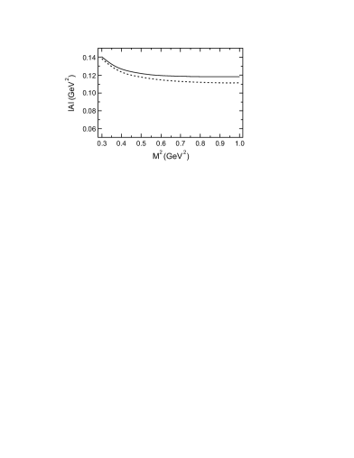
Figure 1: Coupling of the $\eta$ to the pseudoscalar current as a function of the Borel parameter $M$, for $m_{s}=0.133$ GeV. The solid curve corresponds to the higher threshold $s_{0}=(0.95\;{\rm GeV})^{2}$, the dashed curve corresponds to $s_{0}=(0.9\;{\rm GeV})^{2}$.

The strange quark mass is chosen in the range $m_{s}=0.125-0.140$ GeV, obtained in the same QCD sum-rule framework [11]. The threshold is chosen below the $\eta^{\prime}$ pole and varied between $s_{0}=0.9^{2}-0.95^{2}$ GeV².

Since the Borel parameter has no physical meaning, we require that the result does not depend on it. This is achieved by finding a “stability window”, i.e. an interval of values of $M^{2}$, where the outcome of the sum-rule is almost independent on $M^{2}$. Such a window is usually sought in a restricted interval of values of the Borel parameter chosen by requiring that the perturbative contribution is at least 20 $\%$ of the continuum (which corresponds to considering the integral in the perturbative term up to infinity rather than up to $s_{0}$), which produces an upper bound on the Borel parameter: $M^{2}\leq 1$ GeV². Additionally requiring that the perturbative term is greater than the non-perturbative contribution, the lower bound: $M^{2}\geq 0.5$ GeV², is obtained. Then, the stability window for $M^{2}$ in $[0.8,1]$ GeV² can be selected.

In figure 1 we plot the sum-rule (22) for $m_{s}=0.133$ GeV, which corresponds to the central value of the range of values adopted in the analysis. Taking into account the uncertainty on $m_{s}$, we obtain:

$$|A|=(0.115\pm 0.004)\;{\rm GeV}^{2}\;.$$ (23)

Some comments are in order on the accuracy of the result (23). This has been obtained at leading order in perturbative QCD, as with all the results presented in this paper. Consequently, the uncertainty affecting the determination (23) should be taken modulo the neglect of $\alpha_{s}$ corrections, the role of which we comment on later.

Another source of uncertainty is linked to the choice of the strange quark mass. It should be stressed that the value of this parameter is quite controversial. On the one hand, lattice determinations seem to point towards lower values of $m_{s}$ (for recent reviews see e.g. [12]); on the other hand, results obtained in other approaches indicate higher values [13]. As for QCD sum rules, the result in [11] exploits an accurate determination of the hadronic spectral function based on experimental information on the $K\pi$ system including a non-resonant component in addition to the resonances in the $I=1/2$ channel. In [11] it has been shown that the effect of this non-resonant contribution is a reduction in the spectral function, with a consequent lowering of the value of $m_{s}$ with respect to previous QCD sum rule determinations [14]. We have therefore chosen to adopt the result of [11] at first for consistency, i.e. using a result obtained by the same technique, but also because such a value for $m_{s}$ falls in the middle of the existing range. Moreover, the value ${\bar{m}}_{s}$(1 GeV)=0.125 GeV obtained in [11] could be considered as a lower bound on this parameter, since further experimental information could be added to improve the sum rule further. Consistently, we have used the range for ${\bar{m}}_{s}$ of 0.125-0.140 GeV quoted above. The result (23) turns out to be quite stable. Indeed, we have explicitly checked that using still higher values for $m_{s}$ (up to $0.160$ GeV) would produce little change.

Let us now consider:

$$<0|{\overline{s}}i\gamma_{5}s|\eta^{\prime}>=A^{\prime}\;\;\;.$$ (24)

An analogous calculation gives:

$$(A^{\prime})^{2}e^{-{m_{\eta^{\prime}}^{2}\over M^{2}}}+A^{2}e^{-{m_{\eta}^{2}\over M^{2}}}={3\over 8\pi^{2}}\int_{4m_{s}^{2}}^{s_{0}^{\prime}}ds~{}s~{}\sqrt{1-{4m_{s}^{2}\over s}}e^{-{s\over M^{2}}}$$ (25)

$$- m_{s}e^{-{m_{s}^{2}\over M^{2}}}\Bigg{[}<{\overline{s}}s>\Bigg{(}1-{m_{s}^{2}\over M^{2}}+{m_{s}^{4}\over M^{4}}\Bigg{)}+{1\over M^{2}}<{\overline{s}}g\sigma Gs>\Bigg{(}1-{m_{s}^{2}\over 2M^{2}}\Bigg{)}\Bigg{]}\;\;\;,$$

where we have raised the effective threshold up to $s_{0}^{\prime}$ in such a way as to pick up the $\eta^{\prime}$ pole too: $s_{0}^{\prime}=(1.44,1.55)$ GeV². Using $m_{\eta^{\prime}}=0.958$ GeV and fixing the stability window for $M^{2}$ to be $[1.2,2]$ GeV², we obtain:

$$|A^{\prime}|=(0.151\pm 0.015)\;{\rm GeV}^{2}\;.$$ (26)

We shall use the results (23), (26) in the next section. Though we cannot actually establish the sign of $A$, $A^{\prime}$ from the sum rule, we assume that $A\cdot A^{\prime}>0$.

4 Radiative $\phi\to\eta\gamma$ and $\phi\to\eta^{\prime}\gamma$ decays

Having found the key matrix elements $A$ and $A^{\prime}$ of (23), (26), we now consider the three-point functions defined by

$$<\eta(q_{2})|{\overline{s}}\gamma^{\nu}s|\phi(q_{1},\epsilon_{1})>=F(q^{2})~{}\epsilon^{\nu\alpha\beta\delta}(q_{1})_{\alpha}(q_{2})_{\beta}(\epsilon_{1})_{\delta}$$ (27)

($q=q_{1}-q_{2}$). In order to compute the $\phi\to\eta\gamma$ decay, we need the coupling $g=-{1\over 3}F(0)$, obtained for a real photon coupling to a strange quark. We consider the three-point function:

$$\Pi_{\mu\nu}(q_{1}^{2},q_{2}^{2},q^{2})=i^{2}\int d^{4}x~{}d^{4}y~{}e^{-iq_{1}\cdot x}\,e^{iq_{2}\cdot y}<0|T[J_{5}^{s}(y)J_{\nu}(0)J_{\mu}(x)]|0>$$ (28)

where $J_{5}^{s}$ has been defined above and $J_{\nu}={\overline{s}}\gamma_{\nu}s$ is the vector current. The correlator (28) can be written as:

$$\Pi_{\mu\nu}(q_{1}^{2},q_{2}^{2},q^{2})=\Pi(q_{1}^{2},q_{2}^{2},q^{2})\,\epsilon_{\mu\nu\alpha\beta}(q_{1})^{\alpha}(q_{2})^{\beta}$$ (29)

and a QCD sum-rule can be built up for the structure $\Pi(q_{1}^{2},q_{2}^{2},q^{2})$. The method closely follows the one described for the two-point sum-rule. We assume $\Pi(q_{1}^{2},q_{2}^{2},q^{2})$ obeys a dispersion relation in both the variables $q_{1}^{2},q_{2}^{2}$:

$$\Pi(q_{1}^{2},q_{2}^{2},q^{2})={1\over\pi^{2}}\int ds_{1}\int ds_{2}{\rho(s_{1},s_{2},q^{2})\over(s_{1}-q_{1}^{2})(s_{2}-q_{2}^{2})}\;,$$ (30)

with possible subtractions. Such a representation is true at each order in perturbation theory and, as is standard in QCD sum rule analyses, it is assumed to hold in general. In this case the spectral function contains, for low values of $s_{1}$, $s_{2}$, a double $\delta-$function corresponding to the transition $\phi\to\eta$. Extracting this contribution, we can write:

$$\Pi(q_{1}^{2},q_{2}^{2},q^{2})={AF(q^{2})m_{\phi}f_{\phi}\over(m_{\phi}^{2}-q_{1}^{2})(m_{\eta}^{2}-q_{2}^{2})}+{1\over\pi^{2}}\int_{s_{01}}^{\infty}ds_{1}\int_{s_{02}}^{\infty}ds_{2}\,{\rho^{had}(s_{1},s_{2},q^{2})\over(s_{1}-q_{1}^{2})(s_{2}-q_{2}^{2})}\;,$$ (31)

where subtractions are neglected as later they will vanish on taking a Borel transform. The parameter $A$ appearing in the previous equation is just the coupling of the $\eta$ to the pseudoscalar current, computed in section 3. Deriving an OPE-based QCD expansion for $\Pi$ for large and negative $q_{1}^{2}$, $q_{2}^{2}$ and $q^{2}$, one can write:

$$\Pi(q_{1}^{2},q_{2}^{2},q^{2}) = {1\over\pi^{2}}\int_{4m_{s}^{2}}^{\infty}ds_{1}\int_{4m_{s}^{2}}^{\infty}ds_{2}{\rho^{QCD}(s_{1},s_{2},q^{2})\over(s_{1}-q_{1}^{2})(s_{2}-q_{2}^{2})}$$ (32)

$$+ c_{3}<{\overline{s}}s>+c_{5}<{\overline{s}}g\sigma Gs>+...\;\;.$$

Invoking quark-hadron global duality as before, we arrive at the sum-rule:

$${AF(q^{2})m_{\phi}f_{\phi}\over(m_{\phi}^{2}-q_{1}^{2})(m_{\eta}^{2}-q_{2}^{2})} = {1\over\pi^{2}}\int_{D}ds_{1}ds_{2}{\rho^{QCD}(s_{1},s_{2},q^{2})\over(s_{1}-q_{1}^{2})(s_{2}-q_{2}^{2})}$$ (33)

$$+ c_{3}<{\overline{s}}s>+c_{5}<{\overline{s}}g\sigma Gs>+...\;\;.$$

where the domain $D$ should now also satisfy the kinematical constraints specified below. After a double Borel transform in the variables $-q_{1}^{2}$ and $-q_{2}^{2}$, we obtain:

$$A\;F(q^{2})m_{\phi}f_{\phi} = e^{{m_{\phi}^{2}\over M_{1}^{2}}}e^{{m_{\eta}^{2}\over M_{2}^{2}}}\Bigg{\{}\int ds_{1}\int ds_{2}e^{-{s_{1}\over M_{1}^{2}}}e^{-{s_{2}\over M_{2}^{2}}}{3m_{s}\over\pi^{2}\sqrt{\lambda(s_{1},s_{2},q^{2})}}$$

$$+e^{-{m_{s}^{2}\over M_{1}^{2}}}e^{-{m_{s}^{2}\over M_{2}^{2}}}\Bigg{[}<{\overline{s}}s> \left(2-{m_{s}^{2}\over M_{1}^{2}}-{m_{s}^{2}\over M_{2}^{2}}+{m_{s}^{4}\over M_{1}^{4}}+{m_{s}^{4}\over M_{2}^{4}}+{m_{s}^{2}(2m_{s}^{2}-q^{2})\over M_{1}^{2}M_{2}^{2}}\right)$$

$$+<{\overline{s}}g\sigma Gs> \left({1\over 6M_{1}^{2}}+{2\over 3M_{2}^{2}}-{m_{s}^{2}\over 2M_{1}^{4}}-{m_{s}^{2}\over 2M_{2}^{4}}+{(2q^{2}-3m_{s}^{2})\over 3M_{1}^{2}M_{2}^{2}}\right)\Bigg{]}\Bigg{\}}$$ (34)

The integration domain $D$ over the variables $s_{1},s_{2}$ depends on the value of $q^{2}$ and is given by $D=D_{1}\cup D_{2}$ where:

• $(-q^{2})>s_{02}-4m_{s}^{2}$

  $D_{1}$: $(s_{2})_{-}\leq s_{2}\leq s_{02}$          $4m_{s}^{2}\leq s_{1}\leq s_{01}$

• $(-q^{2})<s_{02}-4m_{s}^{2}$

  $$D_{2}:(s_{2})_{-}\leq s_{2}\leq(s_{2})_{+}\;\;\;\;\; 4m_{s}^{2}\leq s_{1}\leq(s_{1})_{-}$$

  $$(s_{2})_{-}\leq s_{2}\leq s_{02}\;\;\;\;\; (s_{1})_{-}\leq s_{1}\leq s_{01}$$ (35)

with:

$$(s_{2})_{\pm}={2m_{s}^{2}q^{2}+(2m_{s}^{2}-q^{2})s_{1}\pm\sqrt{s_{1}q^{2}(q^{2}-4m_{s}^{2})(s_{1}-4m_{s}^{2})}\over 2m_{s}^{2}}$$ (36)

$$(s_{1})_{\pm}={2m_{s}^{2}q^{2}+(2m_{s}^{2}-q^{2})s_{02}\pm\sqrt{s_{02}q^{2}(q^{2}-4m_{s}^{2})(s_{02}-4m_{s}^{2})}\over 2m_{s}^{2}}\;.$$ (37)

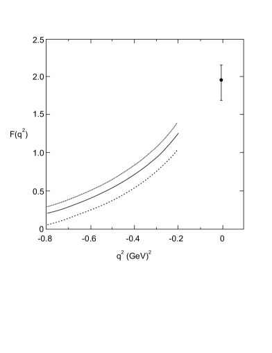
Figure 2: Form factor $F(q^{2})$ obtained varying the input parameters in the sum rule (34). The isolated point on the right is the result of an extrapolation. The extrapolation of the solid curve gives the central point on the right, corresponding to the result (38).

Since we consider the form-factor $F(q^{2})$ for arbitrary negative values of $q^{2}$, we could perform a double Borel transform in the two variables $Q_{1}^{2}=-q_{1}^{2}$ and $Q_{2}^{2}=-q_{2}^{2}$, which allows us to remove single poles in the $s_{1}$ and $s_{2}$ channels (“parasitic” terms) from the sum-rule. Our procedure is therefore to compute the form-factor $F(q^{2})$ and then to extrapolate the result to $q^{2}=0$. Strictly speaking, since we only know the magnitude of $A$ in (33), it is the modulus of $F(q^{2})$ that is determined. In the numerical analysis we use: $m_{\phi}=1.02$ GeV, $f_{\phi}=0.234$ GeV (obtained from the experimental datum on the decay to $e^{+}e^{-}$ [15]). We compute the result for two values of the $\phi$ threshold: $s_{01}=1.8,1.9$ GeV². $s_{02}$ coincides with the $\eta$ threshold chosen as we did for the two point function in section 3.

The outcome of the sum rule is depicted in figure 2. Varying all the parameters entering in the sum rule we obtain a region delimited by the dashed and the dotted curves in this figure: they correspond to the set of parameters giving the highest and the lowest curve analytically defined by (34). The resulting form factor shows a behaviour in $-q^{2}$ in the region $(-0.8,-0.2)$ GeV² which can be fitted by a parabolic function. The extrapolation to $q^{2}=0$ gives:

$$|g|={F(0)\over 3}=(0.66\pm 0.06)\,{\rm GeV}^{-1}\;.$$ (38)

The central value in (38) corresponds to the extrapolation of the solid line in figure 2. The uncertainty range in $|g|$, as obtained by the extrapolation procedure, is displayed in the same figure.

We can now use this result to compute the $\phi\to\eta\gamma$ decay width:

$$\Gamma(\phi\to\eta\gamma)={\alpha g^{2}\over 24}\Big{(}{m_{\phi}^{2}-m_{\eta}^{2}\over m_{\phi}}\Big{)}^{3}\;,$$ (39)

and, using $\Gamma(\phi)=4.43$ MeV [15], we obtain:

$${\cal B}(\phi\to\eta\gamma)=(1.15\pm 0.2)\%\;,$$ (40)

which compares favourably with the experimental outcome: ${\cal B}(\phi\to\eta\gamma)=(1.18\pm 0.03\pm 0.06)\%$ [4].

We can extend the previous analysis to the channel with the $\eta^{\prime}$ in the final state. The derivation of the sum-rule is straightforward:

$$A^{\prime}\;F^{\prime}(q^{2})m_{\phi}f_{\phi}e^{-{m_{\eta^{\prime}}^{2}\over M_{2}^{2}}}+A\;F(q^{2})m_{\phi}f_{\phi}e^{-{m_{\eta}^{2}\over M_{2}^{2}}}=$$ (41)

$$= e^{{m_{\phi}^{2}\over M_{1}^{2}}}\Bigg{\{}\int ds_{1}\int ds_{2}e^{-{s_{1}\over M_{1}^{2}}}e^{-{s_{2}\over M_{2}^{2}}}{3m_{s}\over\pi^{2}\sqrt{\lambda(s_{1},s_{2},q^{2})}}$$

$$+ e^{-{m_{s}^{2}\over M_{1}^{2}}}e^{-{m_{s}^{2}\over M_{2}^{2}}}\Bigg{[}<{\overline{s}}s>\left(2-{m_{s}^{2}\over M_{1}^{2}}-{m_{s}^{2}\over M_{2}^{2}}+{m_{s}^{4}\over M_{1}^{4}}+{m_{s}^{4}\over M_{2}^{4}}+{m_{s}^{2}(2m_{s}^{2}-q^{2})\over M_{1}^{2}M_{2}^{2}}\right)$$

$$+ <{\overline{s}}g\sigma Gs>\left({1\over 6M_{1}^{2}}+{2\over 3M_{2}^{2}}-{m_{s}^{2}\over 2M_{1}^{4}}-{m_{s}^{2}\over 2M_{2}^{4}}+{(2q^{2}-3m_{s}^{2})\over 3M_{1}^{2}M_{2}^{2}}\right)\Bigg{]}\Bigg{\}}$$

The integration region is the same as before with the substitution: $s_{02}\to s_{02}^{\prime}=s_{0}^{\prime}$ (as in the two point sum-rule of section 3). We then obtain:

$$|g^{\prime}|={F^{\prime}(0)\over 3}=(1.0\pm 0.2)\;{\rm GeV}^{-1}$$ (42)

which yields

$${\cal B}(\phi\to\eta^{\prime}\gamma)=(1.18\pm 0.4)~{}10^{-4}\;.$$ (43)

The experimental datum is: ${\cal B}(\phi\to\eta^{\prime}\gamma)=(0.82^{+0.21}_{-0.19}\pm 0.11)~{}10^{-4}$ [4], completely compatible with our result (43).

These results have been derived without including QCD radiative corrections. In principle, each term in the OPE could be computed as an expansion in powers of $\alpha_{s}$, supplementing the non-perturbative expansion with short-distance corrections. This would display the correct scale and scheme dependence for the hadronic quantities, such as the coupling of the $\eta$ and $\eta^{\prime}$ to the currents considered in our analysis. The calculation of QCD corrections is a difficult task well beyond the scope of the present paper. However, we would like to comment on the possible role of such terms.

As far as the two point sum rule is concerned, ${\cal O}(\alpha_{s})$ contributions have been computed [24]. At a typical scale $\mu=1$ GeV, these corrections are sizeable, indicating that still higher orders may also be important. On the other hand, the main goal of the present analysis is the computation of $\phi$ radiative decays. These results are obtained from the ratio of three point to two point sum rules. The most reliable procedure in this case is to compute consistently the three point and two point correlators at the same order in $\alpha_{s}$. The uncertainty due to the neglect of higher order corrections should be reduced due to a cancellation in the ratio.

This expectation is fulfilled, for example, in the calculation using QCD sum rules of the Isgur-Wise function [25], describing in the heavy quark limit the $B\to D^{(*)}$ semileptonic transitions. In this case, though the ${\cal O}(\alpha_{s})$ corrections are large for the two point sum rules [26], explicit calculation of the three point correlator shows the expected cancellation, i.e. the modest role of radiative corrections in the outcome. In this particular case, the result is expected, at least at the zero recoil point, by symmetry requirements. However, this cancellation works in more general situations, such as the one presented in [27], where the universal form factor describing the $B$ transitions to orbitally excited charmed mesons was computed at order $\alpha_{s}$ by the same method. Again, although the two point correlator received important corrections, the ratio ot three to two point functions is quite stable.

In the light of this discussion, our results for the decay constants, eqs. (23),(26), should be considered to be estimates, the uncertainties in which do not take into account possibly sizeable radiative corrections. On the other hand, the outcome for radiative $\phi$ decays, eqs. (40), (43), should be viewed as much more accurate.

Indeed, the predictions for the branching ratios in (40) and (43) are the major results of this paper. They are quite independent of any mixing scheme for the $\eta$ and $\eta^{\prime}$. Nevertheless, adopting the mixing scheme in the flavour basis described in section 2, it is possible to derive the relation:

$$R={{\cal B}(\phi\to\eta\gamma)\over{\cal B}(\phi\to\eta^{\prime}\gamma)}=\Bigg{(}{m_{\phi}^{2}-m_{\eta}^{2}\over m_{\phi}^{2}-m_{\eta^{\prime}}^{2}}\Bigg{)}^{3}\tan^{2}\phi_{s}$$ (44)

from which we get $\phi_{s}=(34\pm^{8}_{6})^{o}$. The experimental ratio would give: $\phi_{s}=(39.0\pm^{7.5}_{5.5})^{o}$.

As mentioned in the introduction, the results obtained can, in principle, provide us with information about the magnitude of the WZW term, which represents an OZI-rule violating contribution to the effective lagrangian. The strength of this term is parametrized by a constant $\Lambda_{3}$ and is determined by the values of the couplings $g$ and $g^{\prime}$. For example, in [5] it is found:

$$g={3m_{\phi}\over 2\pi^{2}f_{\phi}}\left({1\over 6}{\cos\phi_{s}\sin\phi_{V}\over f_{q}}+{1\over 3}{\sin\phi_{q}\over f_{s}}+{\Lambda_{3}\over 3\sqrt{3}}{\sin\theta_{8}\over f_{0}}\right)\;\;,$$ (45)

where $\phi_{V}$ is the mixing angle in the $\phi-\omega$ system. We assume this formula to estimate the size of $\Lambda_{3}$. Unfortunately, the combined effect of the uncertainties affecting the parameters entering (45) allows us no more definite conclusion than $\Lambda_{3}\simeq 2\pm 4$. Precise measurements of $\phi$ radiative decays to $\eta$ and $\eta^{\prime}$ at KLOE [3] will do better.

Let us now compare our results with previous determinations. In ref. [16] the chiral anomaly prediction at $q^{2}=0$ and the vector meson dominance are exploited to derive the couplings $g=g_{\phi\eta\gamma}$ and $g^{\prime}=g_{\phi\eta^{\prime}\gamma}$. A single angle mixing framework in the octet-singlet basis is assumed and the corresponding coupling constants $f_{0}$, $f_{8}$ are derived from the experimental data on the decays $\eta\to\gamma\gamma$ and $\eta^{\prime}\to\gamma\gamma$ and used as an input to derive $g$ and $g^{\prime}$ as a function of the mixing angle. In [8] this approach is extended to the quark-flavour mixing scheme with the result: $g=0.78$ GeV^-1 and $g^{\prime}=0.95$ GeV^-1. On the other hand, an energy-dependent mixing scheme is adopted in [17], with the result: $g=(0.73\pm 0.06)$ GeV^-1 and $g^{\prime}=(0.83\pm 0.06)$ GeV^-1. Alternatively, Ref. [18] exploits the hidden local symmetry approach, together with the inclusion of various $SU(3)$ symmetry breaking [19, 20] to obtain $g=g^{\prime}=0.70$ GeV^-1. As can be observed, the various approaches seem to agree quite well for the decay with the $\eta$ in the final state, while the results have a larger spread in the case of the $\eta^{\prime}$. For a more comprehensive survey of results we refer to [5].

5 $\eta$ and $\eta^{\prime}$ couplings to axial-vector currents using two-point sum-rules

Our study of $\phi$ radiative decays to $\eta$ and $\eta^{\prime}$ require no knowledge of $\eta-\eta^{\prime}$ mixing, only the coupling to strange quarks is needed. However, using similar techniques, we can investigate their decay constants in both the strange and non-strange sectors and so deduce the mixing pattern within errors. This is the purpose of this section. We begin by considering the correlator

$$\Pi_{\mu\nu}(q^{2})=i~{}\int d^{4}x~{}e^{iq\cdot x}<0|T[J_{5\mu}^{s}(x)J_{5\nu}^{s}(0)]|0>$$ (46)

Following the procedure already outlined above, we obtain the sum-rule:

$$(f_{\eta}^{s})^{2}=e^{m_{\eta}^{2}\over M^{2}}\Bigg{[}{1\over\pi}\int_{4m_{s}^{2}}^{s_{0}}ds~{}e^{-{s\over M^{2}}}\rho^{pert}(s)+{2m_{s}\over M^{2}}<{\overline{s}}s>e^{-{m_{s}^{2}\over M^{2}}}\Bigg{]}$$ (47)

where:

$$\rho^{pert}(s)={1\over 4\pi}\sqrt{1-{4m_{s}^{2}\over s}}\quad{2m_{s}^{2}+s\over s}$$ (48)

(in this case the $d=5$ contribution vanishes).

Figure 3: Constant $f_{\eta}^{s}$ as a function of the Borel parameter $M$ for $m_{s}=0.133$ GeV. The solid curve corresponds to $s_{0}$=(0.95 GeV)², the dashed one to $s_{0}$=(0.9 GeV)².

The allowed range for the Borel parameter, obtained according to the above criteria, is: $0.35$ GeV${}^{2}\leq M^{2}\leq 3.5$ GeV², and the further stability window is found in $[2,3.5]$ GeV². The result is depicted in figure 3, for the value $m_{s}=0.133$ GeV. Taking into account the uncertainty in $m_{s}$ too we get:

$$f_{\eta}^{s}=(0.13\pm 0.01)\;{\rm GeV}\;.$$ (49)

In order to determine $f_{\eta^{\prime}}^{s}$ one has to repeat the previous calculation more or less exactly, raising the threshold above the $\eta^{\prime}$ mass and considering the pole contribution of the $\eta$ on the hadronic side of the sum-rule. The result is:

$$(f_{\eta^{\prime}}^{s})^{2}e^{-{m_{\eta^{\prime}}^{2}\over M^{2}}}+(f_{\eta}^{s})^{2}e^{-{m_{\eta}^{2}\over M^{2}}}={1\over\pi}\int_{4m_{s}^{2}}^{s_{0}^{\prime}}ds\,e^{-{s\over M^{2}}}\rho^{pert}(s)+{2m_{s}\over M^{2}}<{\overline{s}}s>e^{-{m_{s}^{2}\over M^{2}}}$$ (50)

where $\rho^{pert}(s)$ is the same as before. In the numerical analysis, $s_{0}^{\prime}$ is varied in the range $(1.2-1.25$ GeV)². The selected stability window for $M^{2}$ is $[2,5]$ GeV². We obtain:

$$f_{\eta^{\prime}}^{s}=(0.12\pm 0.02)\;{\rm GeV}\;.$$ (51)

If we now use the current $J_{5\mu}^{q}$ in the correlator, instead of $J_{5\mu}^{s}$, and we set the up and down quark masses to zero, we can obtain $f_{\eta}^{q}$. The stability window is found for $M^{2}$ in the range $[2,4]$ GeV² with the result

$$f_{\eta}^{q}=(0.144\pm 0.004)\;{\rm GeV}\;.$$ (52)

Raising the threshold, we can also evaluate $f_{\eta^{\prime}}^{q}$, with the result:

$$f_{\eta^{\prime}}^{q}=(0.125\pm 0.015)\;{\rm GeV}\;.$$ (53)

As with the results obtained in section 3 from two-point sum rules, these also represent estimates, derived without radiative QCD corrections.

We can now use the set of results (49), (51), (52), (53) to estimate all the mixing parameters appearing in (6). From the relation ${f_{\eta}^{s}/f_{\eta^{\prime}}^{s}}=\tan\phi_{s}$, one has $\phi_{s}=(46.6^{o}\pm 7^{o})$. Since $f_{\eta}^{s}=f_{s}\sin\phi_{s}$ , a prediction for $f_{s}$ follows: $f_{s}=(0.178\pm 0.004)$ GeV, the central value corresponding to $f_{s}=1.345f_{\pi}$, with $f_{\pi}=0.132$ GeV.

Using the relation: ${f_{\eta^{\prime}}^{q}/f_{\eta}^{q}}=\tan\phi_{q}$, we find $\phi_{q}=(41^{0}\pm 4^{o})$. We can now derive a prediction for $f_{q}$, using $f_{\eta}^{q}=f_{q}~{}\cos\phi_{q}$. We obtain $f_{q}=(0.19\pm 0.015)$ GeV, the central value of which corresponds to $f_{q}\simeq 1.44f_{\pi}$. Let us observe that our results correspond to $|\phi_{s}-\phi_{q}|/(\phi_{s}+\phi_{q})\simeq 0.065$, which confirms the relation put forward in [8] that this ratio should be much less than 1.

If we now turn to the scheme with two mixing angles in the octet-singlet basis, we could exploit the relations (8)-(10) to obtain:

$$\theta_{8}\simeq-8.4^{o}\hskip 28.45274pt \theta_{0}\simeq-13.8^{o}$$

$$f_{8}\simeq 1.44~{}f_{\pi}\hskip 28.45274pt f_{0}\simeq 1.35~{}f_{\pi}\;.$$ (54)

Previous determinations of the parameters calculated above range over large intervals, expecially for those corresponding to (54), i.e. in the octet-singlet mixing scheme. For a comprehensive collection of previous results we again refer to [5]. We only observe that our results for $\phi_{q}$, $\phi_{s}$ are in pretty good agreement with those in refs. [7, 18, 21]. Our outcome for $f_{s}$ also agrees quite well with most of previous results [5], while the result for $f_{q}$ seems somewhat larger than previous determinations.

We can now exploit the results obtained in this section, i.e. the values in (49), (51), together with the predictions (23) and (26), to derive the following matrix elements from (13):

$$\langle 0\left|{\alpha_{s}\over 4\pi}G\tilde{G}\right|\eta\rangle = (0.008\pm 0.004)\,{\rm GeV}^{3}\quad,$$

$$\langle 0\left|{\alpha_{s}\over 4\pi}G\tilde{G}\right|\eta^{\prime}\rangle = (0.072\pm 0.025)\,{\rm GeV}^{3}\;.$$ (55)

Both values in (55) are close to the naive quark model calculation of Novikov et al. [22], particularly that for the $\eta^{\prime}$, which is $f_{\pi}\ m_{\eta^{\prime}}^{2}/\sqrt{3}=0.070$ GeV³. Our result for the $\eta$ is somewhat smaller than the one found in [22]: $f_{\pi}\ m_{\eta}^{2}/\sqrt{6}=0.016$ GeV³. However, their simple quark model result does not take into account $SU(3)_{F}$ breaking corrections. In contrast, ours does. Thus, the matrix elements of (55) are important for the investigation of the structure of the $\eta$ and $\eta^{\prime}$ and their possible glue content [22, 23].

6 Conclusions

We have analysed radiative $\phi\to\eta\gamma$, $\phi\to\eta^{\prime}\gamma$ decays using QCD sum-rules. This analysis required a preliminary calculation of the couplings of the pseudoscalar current to the $\eta$ and $\eta^{\prime}$. The sum-rules are derived without any assumption about $\eta-\eta^{\prime}$ mixing. Though we use only lowest order in QCD perturbation theory, potentially large higher order corrections are expected to cancel between the three and two point correlators, to give results that are in good agreement with the available experimental data on the $\eta$ channel, and are compatible with the Novosibirsk datum for the $\eta^{\prime}$ case. Since the uncertainty in the latter is large, the last word is still left to the experimental improvement at DA$\Phi$NE, for instance.

We have also discussed the issue of $\eta-\eta^{\prime}$ mixing, giving predictions for the parameters describing such mixing in a quark-flavour basis scheme. We observe that the two angles required in such a scheme are quite close to each other. The existing spread of results gives us confidence that new experimental information will shed light on this sector of low-energy physics too.

Acknowledgments

We are most grateful for support from the EU-TMR Programme, Contract No. CT98-0169, EuroDA$\Phi$NE.