Dynamical behavior of spatially inhomogeneous relativistic $\lambda\phi^{4}$ quantum field theory in the Hartree approximation

Abstract

We study the dynamics of a spatially inhomogeneous quantum $\lambda\phi^{4}$ field theory in $1+1$ dimensions in the Hartree approximation. In particular, we investigate the long-time behavior of this approximation in a variety of controlled situations, both at zero and finite temperature. The observed behavior is much richer than that in the spatially homogeneous case. Nevertheless, we show that the fields fail to thermalize in a canonical sense, as expected from analogous results in closely related (mean field) transport theory. We argue that this dynamical approximation is best suited as a means to study the short-time decay of spatially inhomogeneous fields and in the dynamics of coherent quasi-classical inhomogeneous configurations (e.g. solitons) in a background of dynamical self-consistent quantum fluctuations.

I Introduction

In recent years much progress has been made in understanding the real time dynamics of spatially homogeneous quantum field theories. This has been made possible by considering mean field approximations (e.g., Hartree or the large-$N$ limit) to the full quantum dynamics of these systems. The advantage of such techniques is that they permit the approximate evolution of an arbitrarily out-of-equilibrium quantum field theory under many different circumstances, such as in the presence of large mean fields and/or at symmetry breaking phase transitions, where perturbative methods fail.

Numerous applications of this type of dynamics have been considered, ranging from symmetry breaking phase transitions [1], decoherence and dephasing [2], the formation of disoriented chiral condensates at the collisions of relativistic heavy ions [3], to the re-heating and preheating of the early universe [4], to name just a few. Nevertheless, the approximations involved in this kind of evolution lead to two serious limitations, standing in the way of making the results apply to more general and realistic circumstances. The first drawback is that the long-time behavior of the system is incorrect due to the absence of collisional effects. The second is that only spatially homogeneous situations could, until recently [5, 6], be considered. Both limitations are not a matter of principle; they can be overcome with large increases in computational effort, although theoretical progress, e.g., the development of a time-local formulation of the quantum field dynamics including scattering, would be welcomed.

In this paper we lift the constraint on the spatial homogeneity of the system. Mean field theories can be very naturally generalized to spatially inhomogeneous circumstances, allowing the study of the (approximate) evolution of quantum fluctuations in the background of dynamical, spatially dependent fields. This generalization results in a demanding numerical problem, requiring the solution of a large set of coupled partial differential equations. As will be made clear later, the size of the computational effort scales as $L^{2D}$, where $L$ is the linear dimension of the problem and $D$ the number of space dimensions. Thus problems in lower spatial dimensions are significantly more accessible.

One question of great general interest is whether by considering spatially inhomogeneous situations one improves on the long-time properties of the mean field approximation. In particular we will investigate if the long-time regime is in any sense universal and, in particular, if it corresponds to canonical thermal equilibrium. Sallé, Smit and Vink [6] have recently found that, under averaging over an ensemble of certain classes of initial conditions for the mean field, the statistical occupation number of the fluctuations may dynamically approximate a Bose-Einstein distribution over a limited range of times. Although these results are very interesting, we believe that the averaging over ensembles of initial mean fields is not justified from first principles, since the mean field is by definition already the quantum ensemble average one-point function. The potential power of inhomogeneous quantum evolutions is to handle situations where a specific spatially dependent expectation value of the quantum field exists due to some perturbation of thermal equilibrium or of another asymptoticly stable state. Restrictions to particular types of initial conditions defeat the general purpose of the method. For these reasons we will adopt a more general stance here and investigate the main characteristics of the mean field dynamics without any additional ensemble averaging.

We do this in the context of a relativistic $\lambda\phi^{4}$ quantum field theory in $1+1$ dimensions. In section II we define the quantum field theory, and the mean field equations of motion. In section III we make our choice of initial conditions and discuss the renormalization scheme necessary to make the theory independent of the ultraviolet cutoff. We proceed in section IV to analyze the decay of a family of Gaussian spatial profiles. This allows us to investigate the dynamical response of the quantum fluctuation to this field background. We characterize general properties of the dynamics of the mean field and of the quantum fluctuations and pay particular attention to their long-time limit. We then proceed in section V, in the spirit of transport theory, to study the evolution of a mean field small perturbation to a state of thermal equilibrium. Together the results of section IV and V allow us to determine whether the model thermalizes at long times in circumstances of general interest. Finally we present our conclusion and outlook for further applications.

II Theory and definitions

We study the dynamics of a relativistic quantum $\lambda\phi^{4}$ theory in $1+1$ dimensions. We write the Lagrangian density as

$${\cal L}={1\over 2}(\partial_{\mu}\phi)(\partial^{\mu}\phi)-{m^{2}\over 2}\phi^{2}-{\lambda\over 4}\phi^{4}.$$ (1)

The field $\phi$ is taken to be real. We will work in units in which the speed of light $c$ and Boltzmann’s constant $k_{B}$ are unity $c=1,\ k_{B}=1$.

There are several different ways of obtaining mean field approximations to the quantum field theory, by writing truncated effective actions (e.g. in the large $N$ limit [7]), by making a Gaussian variational ansatz in the context of a Schrödinger functional approach [8], or by explicitly expressing higher point field correlation functions in terms of the one- and two-point functions, thus effectively truncating the Dyson-Schwinger hierarchy. While these procedures do not lead to the same approximation to the full thermo(dynamics), the resulting equations share much in common. Below we adopt the familiar Hartree approximation to the dynamical equations for the one- and two-point functions of the quantum field $\phi$. The type of evolution described in this paper generalizes to any other mean field approximation with a similar amount of computational effort.

Following these remarks, we separate the quantum field in a mean field $\varphi\equiv\langle\phi\rangle$ and a fluctuation field $\hat{\psi}$ ($\langle\hat{\psi}\rangle=0$), such that

$$\phi(x,t)=\varphi(x,t)+\hat{\psi}(x,t).$$ (2)

Our mean field approximation (which coincides with the familiar Hartree approximation) corresponds to keeping only the connected two-point function in $\hat{\psi}$. Higher point connected correlation functions of the fluctuations are assumed to be zero. Thus we have, e.g., $\langle\hat{\psi}^{4}\rangle=3\langle\hat{\psi}^{2}\rangle^{2}$. Equations of motion for the mean field and the Wightman two-point function $G^{>}(x,t;x^{\prime},t^{\prime})=\langle\hat{\psi}(x,t)\psi(x^{\prime},t^{\prime})\rangle$ then become

$$\left[\Box+m^{2}+\lambda\varphi^{2}(x,t)+3\lambda G^{>}(x,t)\right]\varphi(x,t)=0,$$ (3)

$$\left[\Box+\chi(x,t)\right]G^{>}(x,t;x^{\prime},t^{\prime})=0,\qquad\chi(x,t)=m^{2}+3\lambda\varphi^{2}(x,t)+3\lambda G^{>}(x,t),$$ (4)

with $\Box=\partial_{t}^{2}-\partial_{x}^{2}$, $G^{>}(x,t;x^{\prime},t^{\prime})=\langle\hat{\psi}(x,t)\hat{\psi}(x^{\prime},t^{\prime})\rangle$ and $G^{>}(x,t)\equiv G^{>}(x=x^{\prime},t=t^{\prime})$.

The relation between the (bosonic) Wightman functions $G^{\stackrel{{\scriptstyle<}}{{>}}}$ and the time ordered (Feynman) two-point function $G_{F}(x,t;x^{\prime},t^{\prime})$ is

$$G^{>}(x,t;x^{\prime},t^{\prime})=G^{<}(x^{\prime},t^{\prime};x,t),\qquad G^{>}(x,t;x^{\prime},t^{\prime})={G^{<}}^{*}(x,t;x^{\prime},t^{\prime}),$$ (5)

$$G_{F}(x,t;x^{\prime},t^{\prime})=\Theta(t-t^{\prime})G^{>}(x,t;x^{\prime},t^{\prime})+\Theta(t^{\prime}-t)G^{<}(x,t;x^{\prime},t^{\prime}),$$ (6)

where $\Theta(t)$ is the usual step function. The advantage of working with the Wightman functions $G^{\stackrel{{\scriptstyle<}}{{>}}}$ is that they obey homogeneous equations of motion.

It is convenient to solve Eqs. (3) by decomposing $G^{>}(x,t;x^{\prime},t^{\prime})$ in a complete orthonormal basis of mode fields, which we shall denote by $\{\psi_{k}(x,t)\}$. The mode index $k$ may be continuous or discrete. In a general context we will denote traces over the basis of field modes as sums over $k$. Then we can write the quantum field $\hat{\psi}(x,t)$ as an expansion in this basis:

$$\hat{\psi}(x,t)=\sum_{k}\left\{a_{k}\psi_{k}(x,t)+a_{k}^{\dagger}\psi_{k}^{*}(x,t)\right\},$$ (7)

where $a_{k},\ a_{k}^{\dagger}$ are the annihilation and creation operators, respectively, obeying canonical commutation relations

$$\left[a_{k},\ a_{q}^{\dagger}\right]=\delta_{kq},\ \left[a_{k},\ a_{q}\right]=\left[a_{k}^{\dagger},\ a_{q}^{\dagger}\right]=0.$$ (8)

Using (7) and (8) and $\langle a_{k}^{\dagger}a_{q}\rangle=\delta_{kq}n_{B}(k)$ we can write $G^{>}(x,t;x^{\prime},t^{\prime})$ as

$$G^{>}(x,t;x^{\prime},t^{\prime})=\sum_{k}\left\{(n_{B}(k)+1)\psi_{k}(x,t)\psi_{k}^{*}(x^{\prime},t^{\prime})+n_{B}(k)\psi_{k}^{*}(x,t)\psi_{k}(x^{\prime},t^{\prime})\right\},$$ (9)

where $n_{B}(k)$ is the Bose-Einstein thermal occupation number distribution

$$n_{B}(k)={1\over e^{\hbar\omega_{k}/T}-1},$$ (10)

with $\omega_{k}$ the energy eigenvalue associated with the eigenfield $\psi_{k}(x,t)$. In particular, the equal-point function $G^{>}(x,t)$ acquires the familiar form

$$G^{>}(x,t)=\sum_{k}\left[2n_{B}(k)+1\right]\psi_{k}(x,t)\psi_{k}^{*}(x,t).$$ (11)

The spectrum reduces to the vacuum as $T\rightarrow 0$, since $n_{B}\rightarrow 0$.

The equation of motion for $G^{>}(x,t;x^{\prime},t^{\prime})$ can now be written in terms of the mode functions $\psi_{k}$:

$$\left[\Box+\chi(x,t)\right]\psi_{k}(x,t)=0,$$ (12)

which must be solved for all $k$. Additionally $\chi(x,t)$ can be expressed entirely in terms of $\varphi$ and $\psi_{k}$ through Eq. (11), so that we obtain a set of self-consistent partial differential equations for the fields $\varphi(x,t)$ and for each of the $\psi_{k}(x,t)$. This set is formally infinite; to obtain a good approximation to the dynamics in the continuum we must take a very large number of mode fields $\psi_{k}(x,t)$, thus the problem becomes demanding in terms of computational resources.

In practice, the fields $\varphi(x,t),\psi_{k}(x,t)$ are evolved on a spatial lattice. Renormalizability requires that the mode fields $\psi_{k}$ must reduce to the vacuum at large $k$ and become plane waves. This limit places a restriction on the modes that can be resolved dynamically: for a spatial lattice of $N$ sites, with spacing $\triangle x$, modes with wavenumber $k>2\pi/\triangle x$ cannot be kept as dynamical fields. Using periodic boundary conditions in space, the $n$th wavenumber is $k_{n}=2\pi n/N\triangle x$. Thus the number of mode functions is restricted to $N$ per linear dimension. Then we see that the computational effort in $D$ space dimensions corresponds to that of solving $N^{D}$ coupled partial differential equations on a grid of size $N^{D}$ points, i.e. it scales as $N^{2D}$ per time step, or like the $D$-dimensional volume squared. This scaling makes the evolution on large spatial lattices in three dimensions very demanding. For the rest of this paper we will be concerned with time evolution of one-dimensional fields.

Finally, we need to specify a basis $\left\{\psi_{k}(x,t)\right\}$, together with the scalar product

$$\left(\psi_{k}(x,t).\psi_{q}(x,t)\right)=i\int dx\left\{\psi_{k}^{*}(x,t)\partial_{t}\psi_{q}(x,t)-\psi_{q}(x,t)\partial_{t}\psi_{k}^{*}(x,t)\right\}.$$ (13)

It follows directly from the form of the equations of motion (3) and (12) that the scalar product (13) is invariant under the dynamics, i.e., $\partial_{t}\left(\psi_{k}(x,t).\psi_{q}(x,t)\right)=0$ for all $k,q$. This guarantees that the orthonormality of the basis, chosen at the initial time, remains valid to all subsequent times, although the set of fields $\psi_{k}$ will evolve away from their initial conditions.

At the initial time, it is convenient to parameterize the set of functions $\psi_{k}$ by

$$\psi_{k}(x,t)=\sqrt{\hbar\over 2\omega_{k}}e^{-i\omega_{k}t}g_{k}(x).$$ (14)

The canonical equal-time commutation relations for the fundamental quantum field $\hat{\psi}(x,t)$

$$\langle\left[\hat{\psi}(x,t),\partial_{t}\hat{\psi}(x^{\prime},t)\right]\rangle=i\hbar\delta^{D}(x-x^{\prime})$$ (15)

must hold. This places a further requirement that the Wronskian condition

$$\psi_{k}(x,t)\partial_{t}\psi_{k}^{*}(x^{\prime},t)-\partial_{t}\psi_{k}(x,t)\psi_{k}^{*}(x^{\prime},t)=i\hbar g_{k}(x)g_{k}^{*}(x^{\prime}),$$ (16)

together with the completeness condition

$$\sum_{k}g_{k}(x)g_{k}^{*}(x^{\prime})=\delta^{D}(x-x^{\prime}),$$ (17)

must be satisfied. In the spatially homogeneous case one chooses $g_{k}(x)$ to be plane waves $g_{k}(x)=e^{ikx}$, which clearly satisfy (16) and (17). Once satisfied at $t=0$, the stationarity of the scalar product also guarantees these properties at later times.

Given (13)-(14), the purely spatial fields $g_{k}(x)$ satisfy the static eigenvalue problem

$$\left[-\nabla_{x}^{2}+\chi(x)\right]g_{k}(x)=\omega_{k}^{2}g_{k}(x).$$ (18)

The scalar product (13) can now be written in terms of $g_{k}$:

$$\left(g_{k}(x).g_{q}(x)\right)=\int dx~{}g_{k}^{*}(x)g_{q}(x),$$ (19)

which is familiar from quantum mechanics. With these definitions orthogonality of the set $\{g_{k}\}$ is equivalent to orthogonality in $\{\psi_{k}\}$.

III Initial conditions and renormalization

To fully specify our initial value problem we need to choose initial conditions for the fields. The initial fields must also be spatially periodic. For the mean field we choose a family of Gaussian profiles

$$\varphi(x,t=0)=\phi_{0}\exp\left[-{x^{2}\over 2A}\right],$$ (20)

where $\phi_{0},A$ are real parameters. In addition we choose the conjugate momentum $\partial_{t}\varphi(x,t=0)=0$, for simplicity. The choice of the set $\psi_{k}$ carries some arbitrarily for small $k$. As we have seen above, only a self-consistent set of modes solved in the background of (20) can supply us with a globally static solution. This type of solution is currently being investigated [9, 10] for specific profiles of $\varphi$.

The simplest possible set of mode fields satisfying all necessary requirements are plane waves

$$g_{k}(x)=e^{ik\cdot x}.$$ (21)

The periodicity of the spatial boundary conditions enforces $k\rightarrow k_{n}=2\pi n/L$. For numerical work we take the corresponding lattice solution with $\omega_{n}=\sqrt{m^{2}+2(1-\cos(k_{n}\triangle x))/\triangle x^{2}}$, where $L=N\triangle x$ is the physical size of the system, $N$ its number of sites and $\triangle x$ the lattice spacing.

Like most quantum field theories, our model as it stands is unphysical, as it collects infinite vacuum contributions as $\triangle x\rightarrow 0$. Simple power counting shows that $\lambda\phi^{4}$ in $1+1$ dimensions is superrenormalizable: there is a single 1-loop logarithmic ultraviolet divergence in the self-energy. There is also an additional quadratic divergence in the energy, characteristic of the free theory.

To see this, consider the vacuum solutions to equation (12). For the purposes of renormalization we can assume $\varphi$ to be spatially homogeneous. We write $\chi$ as

$$\chi=m^{2}_{\Lambda}+3\lambda\varphi^{2}+{3\lambda\over\pi}\int_{0}^{\Lambda}dk~{}|\psi_{k}|^{2}\left[2n_{B}(k)+1\right],$$ (22)

where the bare mass $m^{2}_{\Lambda}$ is understood to be cutoff dependent in a way that will cancel the divergence resulting from the integral.

To define the spectrum of vacuum excitations, we choose $\chi$ to be the mass squared of the excitations, obtained from the curvature of the classical interaction potential at its minimum, $\chi=m^{2}$. Then, without symmetry breaking $\varphi=0$, we obtain the renormalization condition

$$m^{2}=m_{\Lambda}^{2}+{3\lambda\over\pi}\int_{0}^{\Lambda}dk{\hbar\over 2\omega_{k}},$$ (23)

with $\omega_{k}=\sqrt{k^{2}+\chi}=\sqrt{k^{2}+m^{2}}$. This results in

$$m_{\Lambda}^{2}=m^{2}-{3\lambda\over\pi}\int_{0}^{\Lambda}dk{\hbar\over 2\sqrt{k^{2}+m^{2}}},$$ (24)

$$\chi=m^{2}+3\lambda\varphi^{2}+{3\lambda\over\pi}\int_{0}^{\Lambda}dk\left\{|\psi_{k}|^{2}\left[2n_{B}(k)+1\right]-{\hbar\over 2\sqrt{k^{2}+m^{2}}}\right\},$$ (25)

where the last relation is valid at all times. Clearly we need to take $\Lambda\ll T$ to obtain results that are independent of $\Lambda$.

The choice of plane waves for $\{g_{k}(x)\}$, apart from its simplicity, is not ideal, in the sense that the introduction of an inhomogeneous mean field causes the initial choice of basis to shift quickly to adapt to this background. This leads to a fast transient in the spatial profile of the mode functions $\psi_{k}$ over the set of long length scales that characterize the spatial inhomogeneity of the mean field. Consequently, this effect does not change the renormalization, which is an ultraviolet property.

When computing the energy, we have, in addition to the logarithmic self-energy divergence, a quadratic divergence characteristic of the free theory. The total energy has the form

$$E= {1\over 2}\int dx~{}\left\{|\partial_{t}\varphi(x)|^{2}+|\nabla\varphi(x)|^{2}+m^{2}\varphi(x)^{2}+{\lambda\over 2}\varphi(x)^{4}\right.$$ (27)

$$\left.+\left(m^{2}+3\lambda\varphi^{2}+{3\over 2}\lambda G^{>}(x)\right)G^{>}(x)+\int{d{\bf k}\over 2\pi}~{}\left[|\nabla\psi_{k}(x)|^{2}+|\partial_{t}\psi_{k}(x)|^{2}\right]\right\}.$$

The quadratic divergence arises from the last integral in (27). To remove it we need to subtract the vacuum contribution to this term

$$\Delta E={\hbar\over\pi}\int^{\Lambda}_{0}dk~{}\left[{k^{2}+\omega_{k}^{2}\over 2\omega_{k}}\right]\sim{\hbar\over\pi}\int^{\Lambda}dk~{}k$$ (28)

which is clearly a quadratically divergent integral with the ultraviolet cutoff $\Lambda$. To render the energy finite it is sufficient to subtract the ultraviolet behavior of (28). By subtracting the full integral in (28) we impose the renormalization condition that the physical energy at zero temperature is contained exclusively in the profile of the mean field $\varphi$.

We are now ready to study the non-equilibrium evolution of the quantum fields.

IV The time evolution of inhomogeneous mean fields

In this section we discuss the dynamical properties of the spatially inhomogeneous Hartree approximation. We solve Eqs. (3) and (12), in the region $[-L/2,L/2]$, with periodic boundary condition in space. We discretize the computational domain into $N+1$ points, with $x_{j}=j\triangle x$, $j=-N/2,-N/2+1,...,0,1,2,...,N/2,$ where $\triangle x=L/N.$ We approximate $G^{>}(x,t)$ using $N$ complex base fields. A fourth-order symplectic integrator with a fixed time step $\triangle t$ was used to advance the solution to the final time $t_{f}$. In the results shown below, $L=128$, $N=1024$, $\triangle t=0.0025$.

As a zeroth-order check, we verified that the total energy is conserved to within $0.001\%$, or one part per 100,000. We have also made a ”convergence study”, where, for one set of initial parameters, we performed the simulations using three different spatial discretization $\triangle x$, and found that the integral features of the solutions are unchanged with refinements of spatial resolutions.

In Figure 1 we show several snapshots of the evolution of an initial Gaussian profile with $\phi_{0}=2.0$, $A=1$, and with parameters $\lambda=0.1$, $\hbar=1$, $m^{2}=1$.

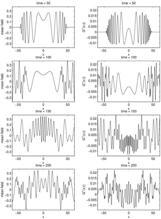
FIG. 1.: Snapshots of the evolution of an initial Gaussian profile with $\phi_{0}=2.0$, $A=1$ and $\lambda=0.1$, $\hbar=m^{2}=1$ in the mean field (left) and $G^{>}(x,t)$ (right).

This situation corresponds to a macroscopic local over-density of the field $\phi$, which could be achieved by turning on an external potential. At $t=0$ the external perturbation is released and the over-density is free to propagate and decay. We see that the Gaussian profile oscillates and decays by emitting wave packets that travel outwards from the perturbation point, both in its own profile, as it would happen in the purely classical case, and in the fluctuation modes, which correspond to particles created by the perturbation.

Because the fluctuations are massive, the medium is dispersive, and different wavelengths propagate outwards at different velocities. We observed that their propagation velocity is bounded by $c=1$, and that shorter wavelengths travel faster, as is apparent in the first few frames of Fig. 1. Meanwhile, some of the energy of the mean field is transfered to the fluctuations, which qualitatively display a similar behavior of wave packets traveling outward from the perturbation point. For late times the wave packets collide due to the periodic nature of the spatial boundary conditions, and continue to propagate back and forth in the computational domain.

An important feature of the evolution is that the mean field does not acquire large power over small spatial scales. In fact, as shown in Fig. 2, most of the power spectrum of the mean field stays contained within the initial Gaussian envelope, although there is some observable enhancement over smaller wavelengths due to the back reaction of the fluctuations.

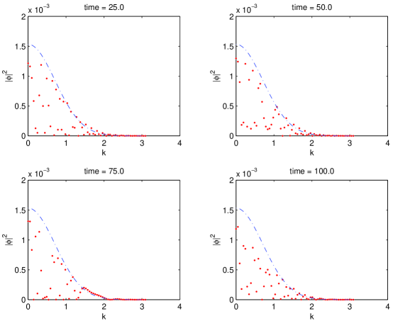
FIG. 2.: Snapshots of the power spectrum of the mean field $\varphi$. The power stays approximately contained within the initial Gaussian envelope (dot-dashed), while decaying slowly as time progresses.

We now turn to the question of the long-time behavior of the dynamics. As a preamble we should keep in mind that our approximation resumes interaction effects that appear at 1-loop order $\sim\lambda$. Consequently we can expect the approximation to be valid up to times $t\sim 1/\lambda=10$, for the case studies shown here. Collisional effects, not included in the Hartree approximation, first appear at two-loops ($\sim\lambda^{2}$) and are necessary to render the evolution physically valid to times of order $t\stackrel{{\scriptstyle>}}{{\sim}}1/\lambda^{2}$. Thus pushing the mean field approximation to large times requires a substantial optimism. Any conclusions it suggests for the properties of the physical system it attempts to describe in this regime should be met with a healthy dose of skepticism.

In any case, as we have discussed above, as time progresses the mean field loses some of its initial energy to the fluctuations. These, however, do not always carry it away efficiently (see also next section), leading at late times to a local dynamical balance between mean field and fluctuations that does not result in the total decay of the former. In this sense we see already that a state of canonical equilibrium is not reached, since the mean field remains non-vanishing. Temporal averages of local mean fields, however, will yield approximately zero. In this sense we may think that the system has reached a state of microcanonical equilibrium and that any local observable, averaged over time, may mimic a corresponding average obtained from the canonical ensemble.

To help us decide whether we may have reached a state of microcanonical equilibrium, we analyze the spectrum of fluctuations $\psi_{k}$. Again, a canonical system in contact with a thermal bath would be expected to thermalize (in the mean field approximation) at a temperature consistent with equipartition. If the system thermalizes, the fluctuation spectrum would satisfy

$$\langle|\psi_{k}|^{2}\rangle={\hbar\over 2\omega_{k}}\left[2n_{B}(\omega_{k})+1\right],\qquad\langle|\pi_{k}|^{2}\rangle={\hbar\omega_{k}\over 2}\left[2n_{B}(\omega_{k})+1\right],$$ (29)

where $\omega_{k}=\sqrt{k^{2}+m^{2}(T)}$, or its form on the spatial lattice, and $\pi_{k}(x,t)=\partial_{t}\psi_{k}(x,t)$. These reduce to their classical Boltzmann forms in the limit of $\hbar\rightarrow 0$

$$\langle|\psi_{k}|^{2}\rangle={T\over\omega^{2}_{k}},\qquad\langle|\pi_{k}|^{2}\rangle=T.$$ (30)

Because of the exponential decay of $n_{B}(\omega_{k})$ for large $\omega_{k}$, the vacuum contribution is typically dominant with $T=0$ initial conditions. We plot instead $\langle|\psi_{k}|\rangle-\langle|\psi_{k}|\rangle_{0}$, by subtracting out the vacuum piece.

$E=0.008426$		$E=0.855148$
$A$	$\phi_{0}$	$A$	$\phi_{0}$
2.00	0.260128	2.00	2.60106
1.00	0.200000	1.00	2.00000
0.50	0.146311	0.50	1.46514
0.25	0.101603	0.20	1.01951

TABLE I.: The height $\phi_{0}$ and variance $A$ of the initial Gaussian mean field $\varphi(x,0)$, Eq. (20) used to generate a family of evolutions with the same energy $E$. The results for the late time fluctuation power spectrum are shown in Figs. 3, 4.

To investigate whether the late time fluctuation power spectrum is in any sense universal we set up a family of initial conditions by varying $\phi_{0}$ and $A$ under the restriction that the renormalized total energy of the system $E$ stays constant, keeping $\lambda=0.1$ fixed. Table I shows the values of $\phi_{0}$ and $A$ used, for two different values of the energy $E$. Fig. 3 shows several late-time fluctuation power spectra for initial Gaussian mean field profiles, while Fig. 4 displays the corresponding spectra of the fluctuation conjugate momenta. After an initial transient, the spectra tend to settle to an approximately time independent profile. Although some of the general features of the several spectra are similar they differ in, for example, amplitude. The fluctuation spectra are reasonably fitted by a power law $\omega^{-\alpha}$, with $2<\alpha<4$, while that of the conjugate momenta may be fitted by a similar power law, but with $1<\alpha<2$.

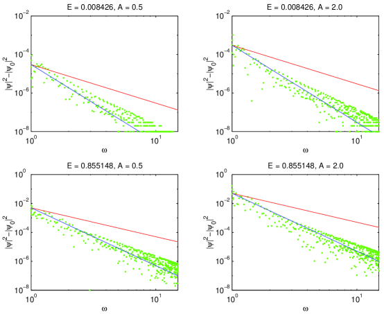
FIG. 3.: Late-time power spectra of the fluctuations $|\psi|^{2}-|\psi(t=0)|^{2}$ (with subtracted vacuum) for various amplitudes and energies, see Table I. Solid lines show $\omega^{-2}$ (upper) and $\omega^{-4}$ (lower) dependences.

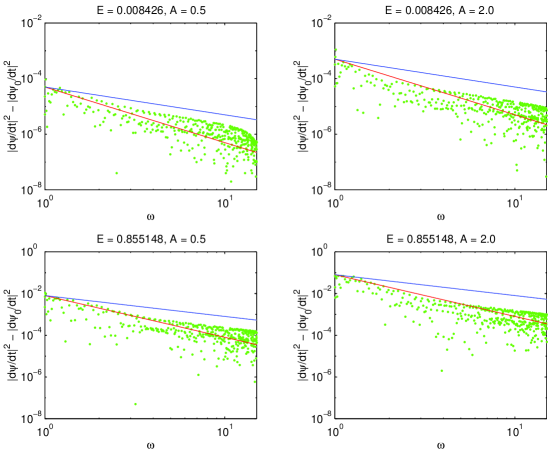
FIG. 4.: Late-time power spectra of the fluctuation conjugate momenta $|\partial_{t}\psi|^{2}-|\partial_{t}\psi(t=0)|^{2}$ (with subtracted vacuum contribution) for various amplitudes and energies, see Table I. Solid lines show $\omega^{-1}$ (upper) and $\omega^{-2}$ (lower) dependences.

These results suggest that at late times the system enters into a dynamical steady state with fluctuation spectra that are uncharacteristic of canonical thermal equilibrium, either in the classical approximation or for quantum fields. Indeed, the characterization of the late-time spectrum as an approximate power law $\omega^{-\alpha}$ with $2<\alpha<4$ suggests that the spectrum of fluctuations is less ultraviolet dominated than in the classical Boltzmann approximation ($\alpha=2$) but more than in its quantum Bose-Einstein form. We never observed exponential suppression of the power spectrum at large $\omega$, as would be expected from quantum canonical equilibrium. Interestingly, this range of power laws shows that the spectrum of fluctuations generated dynamically by the decay of the mean field gives rise to expectation values with no divergence in the limit $k\rightarrow\infty$. If it holds in higher spatial dimensions this is an advantageous feature of the current approximation relative to purely classical field theory. Obtaining truly quantum occupation numbers almost certainly requires the inclusion of quantum scattering effects [11, 12].

The late-time statistical stationarity of the fluctuation power spectra suggests that in its long-time limit the fluctuations may decouple from the evolution. This is what happens in homogeneous mean field theories, where the long-time limit is characterized by $\chi(t)\rightarrow C$, where $C$ is a constant, dependent on the initial conditions. Then the modes $\psi_{k}(t)$ become harmonic oscillators with a corrected frequency. The canonical thermal equilibrium behavior of $\chi(x,t)$ also demands that it becomes a constant in both space and time.

In order to probe this behavior, we show the dynamical evolution of $\chi(x,t)$ and of its power spectrum in Fig. 5.

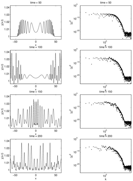
FIG. 5.: The evolution of $\chi(x,t)$ for an initial Gaussian mean field profile with $\phi_{0}=2.0$, $A=1$, $\lambda=0.1$, $m^{2}=1$ and $\hbar=1$ (left) and of its power spectrum (right).

At late times the power spectrum of $\chi$ reaches approximate stationarity. Clearly there is very little power for large $k$, showing that the modes in this regime are essentially decoupled. The approximate stationarity of the power spectrum at small $k$ suggests, however, that the system has reached a statistical dynamical steady-state which does not coincide with canonical thermal equilibrium.

It is clear that initially the mean field induces a strong perturbation in $\chi(x,t)$, which subsequently decays to smaller values in the central region. For late times $\chi(x,t)$ remains a time-dependent, spatially inhomogeneous field, showing that the system continues to exhibit complex dynamics in space-time. This dynamics, however, leads to no significant transport of energy among scales, as evidenced by the approximate stationarity of the fluctuation power spectrum.

Since most non-trivial dynamics happens at early times, we show, in Fig. 6, the very early evolution of $\chi(x,t)$, together with its power spectrum. Recall that a small $\chi$ corresponds to an approximate decoupling of the corresponding mode. As evidenced by Fig. 6, the mean field induces initially significant power over a continuum of large scales. This suggests that the fluctuations have adapted spatially to the non-trivial profile of $\varphi$. The response of the high $k$ modes is selective and can be seen to fall into a distribution of bands. These bands then split into finer and finer ones to become a continuum at late times.

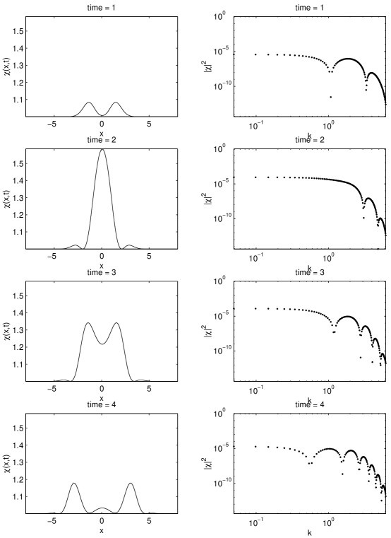
FIG. 6.: Early profiles of $\chi(x,t)$ (left) and corresponding power spectra (right) for the same parameters as in Fig. 5. The higher $k$ modes are populated in bands that later coalesce to form a stable continuum spectrum.

A pattern of excited bands in the fluctuation power spectrum was also observed in the case of the spatially homogeneous evolution of similar theories [13]. Such bands are closely related to exponentially growing solutions of Mathieu’s equation, which describes the behavior of an oscillator whose frequency is a periodic function, supplied in our case by the mean field. In the spatially inhomogeneous case, this pattern is complicated by the fact that the mean field possesses a continuum of frequencies each with a different amplitude. To sketch these parametric resonances, we neglect the fluctuations in the mode equation Eq. (12), since initially this contribution will be small. Then we can write

$$\left[\Box+m^{2}+3\lambda\varphi^{2}(x,t)\right]\psi_{k}(x,t)\simeq 0.$$ (31)

This can be written in Fourier space as

$$\left[\partial_{t}^{2}+(q^{2}+m^{2})\right]\psi_{k}(q,t)+3\lambda\int{dp_{1}\over 2\pi}{dp_{2}\over 2\pi}\varphi(p_{1})\varphi(p_{2})\psi_{k}(q-p_{1}-p_{2},t)=0$$ (32)

The last integral describes mode mixing between the mean field and the fluctuation field $\psi_{k}$. To isolate parametric instabilities we need to further approximate it, by placing $p_{1}=-p_{2}\equiv p$, which results in

$$\left[\partial_{t}^{2}+(q^{2}+m^{2})+3\lambda\bar{\varphi}^{2}\right]\psi_{k}(q,t)\simeq 0,\qquad\bar{\varphi}^{2}=\int dx~{}\varphi^{2}(x)=\int{dp\over 2\pi}~{}|\varphi(p)|^{2},$$ (33)

This equation can be mapped to Mathieu’s equation,

$$\left[\partial_{t}^{2}+a+2\epsilon~{}\cos t\right]\psi_{k}(q,t)=0,$$ (34)

with $a=(q^{2}+m^{2}+3\lambda\bar{\varphi}^{2}(t=0)/2)/(2m)^{2}$, $\epsilon=3\lambda\varphi^{2}(t=0)/8m^{2}$. An instability analysis of Mathieu’s equation with $\bar{\varphi}^{2}(t)\simeq\bar{\varphi}^{2}(t=0)\cos^{2}mt$ predicts instability bands (exponential growing modes) for $a=n^{2}/4$, with $n$ an integer. In terms of the Fourier momentum $q$ this results in $q\simeq m\sqrt{n^{2}-1}=\sqrt{3},\sqrt{8},\sqrt{15},...$, provided $\lambda\bar{\varphi}^{2}(t=0)\ll m^{2}$.

Although this analysis of parametric instabilities is necessarily approximate, we observed that the values for instability modes predicted by Mathieu’s equation are realized to a good approximation in the early dynamics either as maxima or minima in the power spectrum of fluctuations for $k>m$. For small $k$, however, the population of the power spectrum follows a broad continuum presumably seeded not by parametric instabilities but by terms in the mode mixing that act as sources. This behavior is a new feature of the dynamics relative to the spatially homogeneous case. Later, more and more bands appear, resulting in a complicated behavior, until the spectrum reaches a continuum also for large $k$. These aspects of the evolution are quite complex and lie beyond the scope of our present analysis. They will shed light on the detailed mechanisms for energy flow among scales in the model at early times, when the mean field approximation to the dynamics of the quantum fields is justifiable.

V Response around thermal equilibrium

In the previous section we showed some of the general properties of the inhomogeneous mean field evolution starting with families of Gaussian profiles for the mean field and the quantum fluctuations in vacuum. In this section, in the spirit of transport theory, we investigate the properties of the model when perturbed around a self-consistent state of thermal equilibrium.

The mean field equations (3) have as a limiting case a transport mean field theory characterized by a Vlasov equation. The derivation of this transport theory is standard [11] and we will not repeat it here. The transport description is appropriate for small soft disturbances of the system around a stable asymptotic state, usually thermal equilibrium. By solving the corresponding transport theory, one can estimate how the system responds over large spatial scales and long times and, in particular, how and if it returns to thermal equilibrium.

In the context of Boltzmann transport theory, the return to thermal equilibrium is related to a collision kernel resulting from an imaginary part of the self-energy of the field in the medium. For $\lambda\phi^{4}$ the lowest such self-energy is given by the 2-loop sunset diagram, with its imaginary part describing $2\leftrightarrow 2$ particle scattering. Such a self-energy is absent from our description. Thus we may simply expect, as is characteristic of mean field transport descriptions, that disturbances to thermal equilibrium may never decay and that the response and final state of the system is described in terms of characteristics of its initial state (such as its energy), and is therefore not universal.

As we have seen in Eq. (11), thermal initial conditions are easily included through the definition of $G^{>}(x,t)$. To ensure that we start with a self-consistent (static) solution, we must solve the eigenvalue problem corresponding to the state of thermal equilibrium in the mean field approximation. In thermal equilibrium $\varphi=0$ and the tadpole diagram acquire a momentum-independent mass correction $\Delta m^{2}(T)$. The self-consistent solution for the modes $\psi_{k}$ then is in the form of plane waves (14), (21), with frequency $\omega_{k}=\sqrt{k^{2}+m^{2}+\Delta m^{2}(T)}$. The mass correction $\Delta m^{2}(T)$ obeys the gap equation

$$\omega_{k}^{2}\equiv k^{2}+m^{2}+\Delta m^{2}(T),$$ (35)

$$\Delta m^{2}={3\hbar\lambda\over\pi}\int_{0}^{\Lambda}dk~{}\left[{2n_{B}(\omega_{k})+1\over 2\omega_{k}}-{1\over 2\sqrt{k^{2}+m^{2}}}\right],$$ (36)

where we have used a renormalization prescription such that the vacuum tadpole is fully subtracted so that the result coincides with (23), (24) as $T\rightarrow 0$. We implement this solution on our spatial lattice modes $\psi_{k}$ in order to produce a static solution for the numerical evolution. Some sample results are shown in Table II.

$T$	$\Delta m^{2}(T)$
0.0	0.0000
0.5	0.0116
1.0	0.0523
2.0	0.1535
3.0	0.2577
5.0	0.4580
10.0	0.9042

TABLE II.: The thermal mass correction $\Delta m^{2}(T)$ vs. the temperature $T$. The computations used a lattice propagator, and $\lambda=0.1$, $m=1$.

We verified that the solution resulting from this procedure is static in the absence of the mean field or an external perturbation.

An important point to note is that the form of the Bose-Einstein distribution is not essential for the stationarity of the solution. Equation (36) can be satisfied for any other occupation number, provided the integral over $k$ exists. This contrasts once again with the integrals in Boltzmann collisional kernels, for which the Bose-Einstein distribution is usually the unique solution.

We can now explore the response of the fluctuations to a self-consistently evolving mean field or to a static external perturbation. In the examples below we will work at $T=3$, which is a high temperature situation since $T>m(T)=1.12$.

Consider first an external field $\varphi_{\rm ext}$. We assume that a static solution will be reached in this external field and parameterize the linear deviation from thermal equilibrium by generalizing the equilibrium number distribution $n_{B}$ to a general slowly varying function of space and time $n(x,k)$ such that

$$n(x,k)=n_{B}(\omega_{k})+\delta(x){dn_{B}(\omega_{k})\over d\omega_{k}}.$$ (37)

By requiring stationarity of the solution we can conclude that the field $\delta(x)$ is

$$\delta(x)={\varphi_{\rm ext}^{2}\over\int{dk\over 2\pi}{\hbar\over\omega_{k}}{dn_{B}(\omega_{k})\over d\omega_{k}}}.$$ (38)

We can now compare this simple expectation with the result from the evolution. An example is shown in Fig.7 for a Gaussian profile of the form (20) with $\phi_{0}=0.2$ and $A=1$

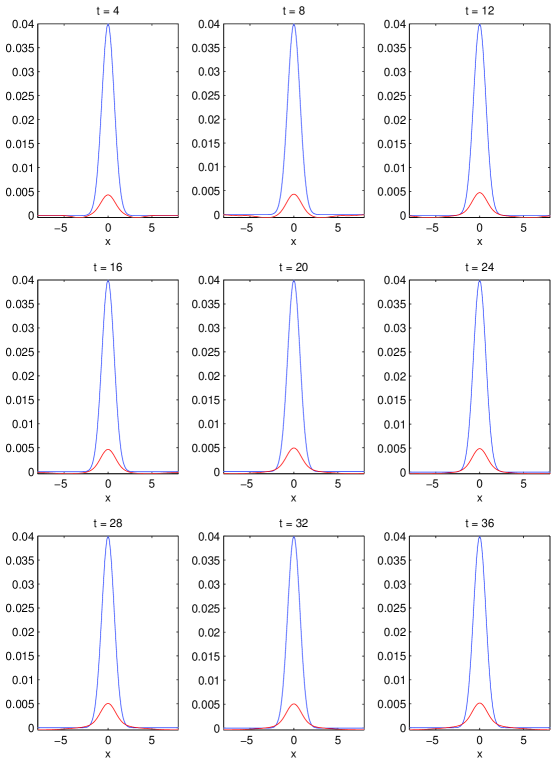
FIG. 7.: $G^{>}(x,t)-G^{>}_{\rm eq}$ (red) showing the response of the fluctuations to an externally imposed Gaussian field $\varphi_{\rm ext}^{2}$ (blue). Eq. (20), with $A=1$ and $\phi_{0}=0.2$ and at temperature $T=3$.

It is striking to see that the fluctuations do not completely cancel out the externally imposed field, and that a globally static solution is not reached at long times. Instead, the fluctuations adapt to the external potential to form a local bound state and some of the energy perturbation introduced at $t=0$, when the mean field was switched on, is carried away by wave packets propagating outwards.

For the same mean field self-consistently evolving with its fluctuations the result is reminiscent of that of section IV, see Fig.8.

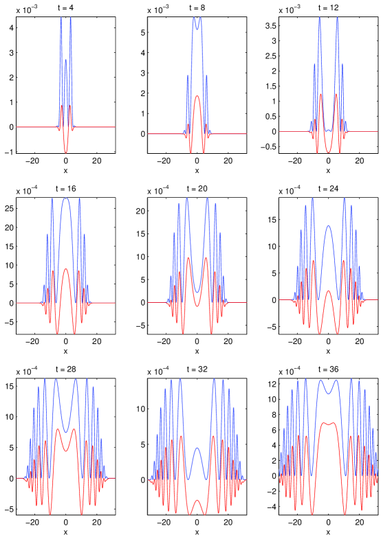
FIG. 8.: $G^{>}(x,t)-G^{>}_{\rm eq}$ (red) showing the response of the fluctuations to a self consistently evolving mean field squared $\varphi(x,t)^{2}$ (blue) started from a Gaussian profile Eq. (20), with $A=1$ and $\phi_{0}=0.2$ and at temperature $T=3$

As in the case of the external perturbation, the self-consistently evolving mean field is partially shielded by fluctuations, but not enough to yield a globally static solution. Instead, as the mean field evolves and its profile changes in space-time, the fluctuations track that change on essentially the same time scale after an initial fast transient.

The properties of self-consistently determined fluctuations in fixed external backgrounds both at zero and finite temperature can be naturally studied in our dynamical approximation. A procedure to compute minimal energy fluctuation modes in these potentials can be easily generated by introducing artificial dissipation in the evolution.

VI Conclusions

We have analyzed the dynamical properties of an inhomogeneous relativistic quantum $\lambda\phi^{4}$ field theory in $1+1$ dimension in the Hartree approximation. We considered the evolution of the fields starting both from a vacuum state and from a state of thermal equilibrium at finite temperature, perturbed by a soft mean field profile.

The resulting evolution can be very complex, opening up many new possibilities in the dynamics of quantum fields arbitrarily away of equilibrium. Spatially inhomogeneous fields are necessary, e.g., in the study of the plasma formed at the ultra-relativistic collision of heavy ions and its subsequent anisotropic cooling and in considering the evolution of charged quantum fields in a mean magnetic field.

The transport of energy from the mean field to the fluctuations proceeds at early times selectively into intervals of spatial scales, which later coalesce to create a continuous spectrum, which becomes almost static at late times. This process, similarly to the spatially homogeneous case, shows effective time irreversibility emerging within the context of a fully unitary quantum field evolution. Although some features of the late fluctuation spectrum may be quite general, others, such as its amplitude, are dependent on the initial state. The dependence of the power spectrum on $\omega$ suggests that the mean field evolution generates occupation numbers that do not reproduce the quantum behavior of the exact quantum field theory but that, at the same time, are better behaved than those of the classical thermal theory. In particular this spectrum leads to no new ultraviolet divergence. It will be interesting if this characteristic holds in higher spatial dimensions where the classical Boltzmann distribution leads to ultraviolet divergent thermal contributions to expectation values of field correlators. Conservation of energy alone seems to suggest that such should be the case.

Neither the mean field nor the spatial homogeneities in the fluctuations decay away completely. At late times the dynamics consists of propagating wave packets in both the mean field and fluctuations. This behavior may have been enhanced in the present study by the fact that there are no massless excitations in the spectrum and therefore there are kinematic thresholds prohibiting further decay. This is a general characteristic of the $N=1$ $\lambda\phi^{4}$ theory considered here. Collectively, the characteristics of the late time evolution, although interesting and an improvement on the homogeneous version of the approximation and on the classical fields, are incompatible with a state of canonical thermal equilibrium. This aspect of the problem will almost certainly require the inclusion of quantum scattering effects [12].

In contrast, physical situations that are dominated by the behavior of (massless) Goldstone modes -such as scalar theories with large $N$- will behave quite differently. The large-$N$ limit of these models can also be studied for spatially inhomogeneous mean fields. Relative to the Hartree approximation it has the added advantage of capturing the correct (mean field) thermodynamics [7, 14]. Unfortunately, the study of the dynamics of symmetry breaking transitions is most interesting in higher spatial dimensions, where, in order to address spatially inhomogeneous situations, a substantial increase in computational effort, relative to that of the present study, will be required.

Our results are complementary to those of Sallé, Smit and Vink [6], who studied the same model under additional averaging over ensembles of mean fields. This ensemble averaging is an additional ingredient not included in the mean-field approximation to the dynamics of the quantum field theory and at face value is not allowed since the mean field already carries the meaning of the quantum ensemble average field expectation value. It may nevertheless be the means to an end -the quantum thermalization of the theory- at the expense of restricting the mean field to particular ensembles. Our results indicate that, without invoking this additional ensemble averaging, the mean-field dynamics does not thermalize for a large class of initial conditions, including the close vicinity of thermal equilibrium.

Because of these shortcomings the dynamical Hartree approximation is best suited to study situations that are not dominated by fluctuations and that are not closely related to a symmetry breaking second order transition. In particular, the evolution of quasi-classical field configurations, such as topological defects and phase interfaces in a background of self-consistent fluctuations, should prove very interesting. The hydrodynamical properties of the model and, in particular, the evolution of the energy momentum tensor in several situations are also being considered.

REFERENCES

- [1] F. Cooper, S. Habib, Y. Kluger, E. Mottola, Phys. Rev. D 55, 6471 (1997); D. Boyanovsky, D. Cormier, H. J. de Vega, R. Holman, Phys. Rev. D 55, 3373 (1997); J. Baacke, K. Heitmann, Phys. Rev. D 62, 105022 (2000).
- [2] S.Habib, Y. Kluger, E. Mottola, J.P. Paz, Phys. Rev. Lett 76, 4660 (1996).
- [3] D. Boyanovsky, H. J. de Vega, R. Holman, Phys. Rev. D 51, 734 (1995); F. Cooper, Y. Kluger, E. Mottola, Phys. Rev. C 54 3298 (1996).
- [4] D. Boyanovsky, M. D’attanasio, H.J. de Vega, R. Holman, D.-S.Lee, Phys.Rev. D 52, 6805 (1995); D. Boyanovsky, H. J. de Vega, R. Holman, J. F. J. Salgado, Phys. Rev. D 56, 1958 (1997).
- [5] G. Aarts and J. Smit, Nucl.Phys. B 555, 355 (1999).
- [6] M. Sallé, J. Smit, J.C. Vink, hep-ph/0012362; hep-ph/0012346.
- [7] F. Cooper, S. Habib, Y. Kluger, E. Mottola, J.P. Paz and P. R. Anderson, Phys. Rev. D 50, 2848 (1994), and references therein.
- [8] F. Cooper, S.-Y. Pi, and P. Stancioff, Phys. Rev. D 34, 3831 (1986).
- [9] D. Boyanovsky, F. Cooper, H. J. de Vega, P. Sodano, Phys.Rev. D 58, 025007 (1998).
- [10] F. Alexander and E. Mottola, in preparation.
- [11] See L. P. Kadanoff and G. Baym, Quantum Statistical Mechanics (W.A.Benjamin, New York, 1962) for the early derivation in the non-relativistic case. The generalization to the relativistic case is immediate and appears frequently in the literature, see e.g. S. Mrowczynski, Phys.Part.Nucl. 30, 419 (1999); Fiz.Elem.Chast.Atom.Yadra 30, 954 (1999) [hep-ph/9805435].
- [12] J. Berges and J. Cox, hep-ph/0006160.
- [13] D. Boyanovsky, H. J. de Vega, R. Holman, J. F. J. Salgado, Phys. Rev. D 54, 7570 (1996).
- [14] G. Amelino-Camelia and S.-Y. Pi, Phys. Rev. D 47, 2356 (1993).