Empirical formulas for the fermion spectra and Yukawa matrices

Abstract

We present empirical relations that connect the dimensionless ratios of fermion masses for the charged lepton, up-type quark and down-type quark sectors: $\left|V_{us}\right|\approx\left[\frac{m_{d}}{m_{s}}\right]^{\frac{1}{2}}\approx\left[\frac{m_{u}}{m_{c}}\right]^{\frac{1}{4}}\approx 3\left[\frac{m_{e}}{m_{\mu}}\right]^{\frac{1}{2}}$ and $\frac{1}{2}\left|\frac{V_{cb}}{V_{us}}\right|\approx\left[\frac{m_{s}^{3}}{m_{b}^{2}m_{d}}\right]^{\frac{1}{2}}\approx\left[\frac{m_{c}^{3}}{m_{t}^{2}m_{u}}\right]^{\frac{1}{2}}\approx\frac{1}{9}\left[\frac{m_{\mu}^{3}}{m_{\tau}^{2}m_{e}}\right]^{\frac{1}{2}}$. Explaining these relations from first principles imposes strong constraints on the search for the theory of flavor. We present a simple set of normalized Yukawa matrices, with only two real parameters and one complex phase, which accounts with precision for these mass relations and for the CKM matrix elements and also suggests a simpler parametrization of the CKM matrix. The proposed Yukawa matrices accommodate the measured CP-violation, giving a particular relation between standard model CP-violating phases, $\beta={\rm Arg}\left[2-e^{-i\gamma}\right]$. According to this relation the measured value of $\beta$ is close to the maximum value that can be reached, $\beta_{\rm max}=30^{\circ}$ for $\gamma=60^{\circ}$. Finally, the particular mass relations between the quark and charged lepton sectors find their simplest explanation in the context of grand unified models through the use of the Georgi-Jarlskog factor.

I Introduction

Any theory of flavor must explain the fermion mass hierarchies as well as the quark mixing angles. Unfortunately, few patterns have been found in the measured values of fermion masses and mixing angles that can guide us in the search for an underlying theory of flavor. One of these, which has been known since 1968 Cabibborelation , is the well known empirical relation between the down-quark mass, the strange-quark mass and the Cabibbo angle,

$$\left|V_{us}\right|\approx\left[\frac{m_{d}}{m_{s}}\right]^{\frac{1}{2}}.$$ (1)

This relation has driven the development of theories of flavor over more than three decades, starting in 1977 with the first attempt to explain it using family symmetries discrete ; reviews . Another quark mass relation that has been known for some time is,

$$\left[\frac{m_{d}}{m_{s}}\right]^{\frac{1}{2}}\approx\left[\frac{m_{u}}{m_{c}}\right]^{\frac{1}{4}}.$$ (2)

Inspired by these two relations, many of the theories of flavor proposed to date have focused on generating Yukawa matrices that are polynomial in powers of $\lambda$, $\lambda\approx\left|V_{us}\right|$, with coefficients of order 1 Froggatt:1978nt . There is a third famous relation. It was argued as early as in 1979 that at momenta larger than $10^{15}$ GeV quark and charged lepton masses are related by,

$$m_{d}=3m_{e},\quad m_{\mu}=3m_{s},$$ (3)

An ingenious method was proposed to account for this relation by the use of SU(5) Clebsch-Gordan coefficients Georgi:1979df . Other than these relations, it is usually claimed that the fermion masses follow scaling laws of the form $(m_{d},m_{s})\simeq(\lambda^{4},\lambda^{2})m_{b}$ in the down-type quark sector, $(m_{u},m_{c})\simeq(\lambda^{8},\lambda^{4})m_{t}$ in the up-type quark sector and $(m_{e},m_{\mu})\simeq(\lambda^{4},\lambda^{2})m_{\tau}$ in the charged lepton sector. As can be easily checked, however, these scaling laws are qualitative and do not survive a precision analysis.

The measurement of the top quark mass in 1995 and the continuous improvement in the extraction of other quark masses during the last decade motivate a more systematic search for precise empirical relations between dimensionless ratios of fermion masses in each fermion sector. There are six independent fermion mass ratios of this kind, two for each fermion sector. It is possible for hidden regularities to manifest themselves more clearly through higher order dimensionless ratios of fermion masses, i.e. ratios of the form $m^{2}_{a}/(m_{b}m_{c})$ or $m^{3}_{a}/(m^{2}_{b}m_{c})$. Indeed, as we show in this paper, there are some interesting patterns underneath the measured values of the fermion masses. These new relations, which are not merely qualitative, are the following,

$$\left|V_{us}\right| \approx \left[\frac{m_{d}}{m_{s}}\right]^{\frac{1}{2}}\approx\left[\frac{m_{u}}{m_{c}}\right]^{\frac{1}{4}}\approx 3\left[\frac{m_{e}}{m_{\mu}}\right]^{\frac{1}{2}},$$ (4)

$$\frac{1}{2}\left|\frac{V_{cb}}{V_{us}}\right| \approx \left[\frac{m_{s}^{3}}{m_{b}^{2}m_{d}}\right]^{\frac{1}{2}}\approx\left[\frac{m_{c}^{3}}{m_{t}^{2}m_{u}}\right]^{\frac{1}{2}}\approx\frac{1}{9}\left[\frac{m_{\mu}^{3}}{m_{\tau}^{2}m_{e}}\right]^{\frac{1}{2}}.$$ (5)

We expect these two basic parameters, which we denote hereafter by $\lambda\approx\left|V_{us}\right|$ and $\theta\approx\frac{1}{2}\left|V_{cb}\right|/\left|V_{us}\right|$, to be connected with the fundamental parameters of the underlying theory of flavor.

This paper is organized as follows. We begin in Sec. II by systematically searching for correlations between dimensionless mass ratios in different fermion sectors up to order 3, i.e. up to ratios of the form $m^{3}_{a}/(m_{b}^{2}m_{c})$. We review in the appendix the calculation of lepton and quark running masses which are used in Sec. II. In Sec.III we analyze Yukawa renormalization corrections that affect the studied mass relations when evolved with the renormalization scale, especially to the ratios including third generation fermion masses. In Sec. IV we show that, as a consequence of these new empirical formulas the fermion mass hierarchies can be expressed as a function of two basic parameters, $\lambda$ and $\theta$. In Sec. V we show, neglecting CP-violation, that the absolute values of the CKM mixing matrix elements can also be expressed as simple functions of the basic parameters $\lambda$ and $\theta$. In Sec. VI we propose, neglecting CP-violation, a simple reconstruction of the quark Yukawa matrices that accounts for the correlations found in the previous sections. In Sec. VII we introduce CP–violation in the textures proposed in Sec. VI and study its predictions for the CP-violating parameters. In Sec. VIII we study the precision predictions for the lighter quark masses, CKM elements and charged lepton masses arising from the texture proposed in Sec. VI. In Sec. IX we point out that the simplest solution to account for the relations between the charged lepton sector and the quark sector can be found in the the extension of the Standard Model $SU(3)_{C}\times SU(2)_{L}\times U(1)_{Y}$ symmetry to the $SU(5)$ symmetry of Georgi and Glashow. In Sec. X we speculate about the characteristics of underlying flavor models that can reproduce these empirical mass relations.

II Correlations between dimensionless fermion mass ratios

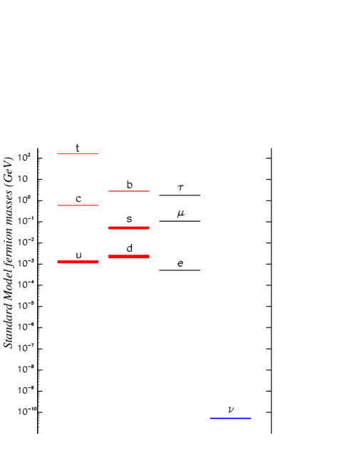
Figure 1: The fermion mass spectra.

In this section we will look for patterns in the dimensionless mass ratios of running fermion masses. Other than the fact that the first fermion generation is lighter than the second and this is lighter than the third generation, there are no other evident regularities in the fermion mass spectra, as can be observed in Fig. 1. Based on the experimental fact that the third generation is much heavier than the first and second generations and that the quark mixing angles are small we hope that there is a simple mechanism of flavor breaking which generates at some higher energy scale a simple structure in the normalized Yukawa matrices. If this is the case it is plausible that at such scale the normalized Yukawa matrices have the form,

$$\widehat{\cal Y}=\left[\begin{array}[]{ccc}0&0&0\\ 0&0&0\\ 0&0&1\\ \end{array}\right]+{\cal O}(\lambda,\theta,\cdot\cdot\cdot),$$ (6)

where $\lambda,\theta,\cdot\cdot\cdot$ represent generically some perturbative flavor breaking parameters, i.e. $\lambda,\theta,\cdot\cdot\cdot\ll 1$, directly related to the underlying theory of flavor. We note that in many flavor models proposed in the literature the flavor breaking is parametrized by a unique parameter $\lambda$. Therefore we expect the fermion mass ratios in each one of the three fermion sectors: up-type quark, down-type quark and charged lepton to be expressed as a simple polynomial functions of the flavor parameters: $\lambda,\theta,\cdot\cdot\cdot$,

$$\widehat{m}_{1} = \frac{m_{1}}{m_{3}}=f_{1}(\lambda,\theta,\cdot\cdot\cdot),$$ (7)

$$\widehat{m}_{2} = \frac{m_{2}}{m_{3}}=f_{2}(\lambda,\theta,\cdot\cdot\cdot).$$ (8)

Let us assume to simplify the discussion that there are only two flavor breaking parameters: $\lambda$ and $\theta$. In this case it would be possible to solve the previous system of equations and obtain expressions for $\lambda$ and $\theta$ as a function of the fermion mass ratios,

$$\lambda = \lambda(\widehat{m}_{1},\widehat{m}_{2}),$$ (9)

$$\theta = \theta(\widehat{m}_{1},\widehat{m}_{2}).$$ (10)

This can be done for each fermion sector separately. This makes plausible that underlying patterns manifest more clearly in higher order mass ratios, even though these can be expressed as a function of the six basic fermion mass ratios. When searching for mass relations between different fermion sectors, it is convenient to calculate ratios of running fermion masses at a common renormalization scale. If there are regularities in the underlying Yukawa matrices, these will be manifested more clearly in the ratios of running fermion masses, not in the ratios of physical masses. Using the running masses that we have calculated in the appendix we obtain dimensionless mass ratios in the charged lepton, up–type quark and down–type quark sectors. We calculate ratios of order 1, $c^{[1]}$, order 2, $c^{[2]}$, and order 3, $c^{[3]}$. These ratios are generically of the form,

$$c_{ab}^{[1]}=\frac{m_{a}}{m_{b}},\quad c_{abc}^{[2]}=\frac{m_{a}^{2}}{m_{b}m_{c}},\quad c_{abc}^{[3]}=\frac{m_{a}^{3}}{m_{b}^{2}m_{c}},$$ (11)

	Charged leptons		Down-type quarks		Up-type quarks
I	$m_{e}/m_{\mu}$	$(4.73711\pm 0.00007)\times 10^{-3}$	$m_{d}/m_{s}$	$(4.4\pm 1.4)\times 10^{-2}$	$m_{u}/m_{c}$	$(2.6\pm 0.8)\times 10^{-3}$
II	$m_{\mu}/m_{\tau}$	$(5.882\pm 0.001)\times 10^{-2}$	$m_{s}/m_{b}$	$(2.4\pm 0.4)\times 10^{-2}$	$m_{c}/m_{t}$	$(3.7\pm 0.6)\times 10^{-3}$
III	$m_{e}m_{\mu}/m^{2}_{\tau}$	$(1.6390\pm 0.0006)\times 10^{-5}$	$m_{d}m_{s}/m^{2}_{b}$	$(2.5\pm 1.0)\times 10^{-5}$	$m_{u}m_{c}/m^{2}_{t}$	$(3.65\pm 1.5)\times 10^{-8}$
IV	$m_{e}^{2}/m_{\mu}m_{\tau}$	$(1.3199\pm 0.0003)\times 10^{-6}$	$m_{d}^{2}/m_{s}m_{b}$	$(4.7\pm 2.5)\times 10^{-5}$	$m_{u}^{2}/m_{c}m_{t}$	$(2.52\pm 1.4)\times 10^{-8}$
V	$m_{\mu}^{2}/m_{e}m_{\tau}$	$12.417\pm 0.002$	$m_{s}^{2}/m_{d}m_{b}$	$0.53\pm 0.26$	$m^{2}_{c}/m_{u}m_{t}$	$(1.45\pm 0.71)$
VI	$m_{e}^{3}/m^{2}_{\mu}m_{\tau}$	$(6.253\pm 0.001)\times 10^{-9}$	$m_{d}^{3}/m^{2}_{s}m_{b}$	$(2.1\pm 1.8)\times 10^{-6}$	$m_{u}^{3}/m^{2}_{c}m_{t}$	$(6.5\pm 5.8)\times 10^{-11}$
VII	$m_{e}^{3}/m_{\mu}m^{2}_{\tau}$	$(3.678\pm 0.001)\times 10^{-10}$	$m_{d}^{3}/m_{s}m^{2}_{b}$	$(5.0\pm 3.7)\times 10^{-8}$	$m_{u}^{3}/m_{c}m^{2}_{t}$	$(2.44\pm 2.0)\times 10^{-13}$
VIII	$m_{\mu}^{3}/m^{2}_{e}m_{\tau}$	$2621.2\pm 0.5$	$m_{s}^{3}/m^{2}_{d}m_{b}$	$12\pm 10$	$m_{c}^{3}/m^{2}_{u}m_{t}$	$(560\pm 455)$
IX	$m_{e}m_{\mu}^{2}/m^{3}_{\tau}$	$(9.640\pm 0.005)\times 10^{-7}$	$m_{d}m_{s}^{2}/m^{3}_{b}$	$(6.0\pm 3.5)\times 10^{-7}$	$m_{u}m^{2}_{c}/m^{3}_{t}$	$(1.4\pm 0.8)\times 10^{-10}$
X	$m_{e}^{2}m_{\mu}/m^{3}_{\tau}$	$(4.567\pm 0.002)\times 10^{-9}$	$m_{d}^{2}m_{s}/m^{3}_{b}$	$(2.7\pm 1.6)\times 10^{-8}$	$m_{u}^{2}m_{c}/m^{3}_{t}$	$(3.5\pm 2.4)\times 10^{-13}$
XI	$m_{\mu}^{3}/m_{e}m^{2}_{\tau}$	$0.7304\pm 0.0002$	$m_{s}^{3}/m_{d}m^{2}_{b}$	$(1.3\pm 0.9)\times 10^{-2}$	$m_{c}^{3}/m_{u}m^{2}_{t}$	$(5.4\pm 3.5)\times 10^{-3}$

Table 1: Dimensionless fermion mass ratios in the charged lepton, up and down–type quark sectors calculated from measured values as explained in the text

where $a,b,c=1,2,3$ are generation indices. Our numerical results are shown in table  1. We have also included uncertainties for the mass ratios, $\Delta c$, calculated using $\Delta c=\left|\partial c/\partial m_{a}\right|\Delta m_{a}$, where $\Delta m_{a}$ are the uncertainties in the determination of running fermion masses. The measured quark and charged lepton masses used as an input in our calculations are explained in detail in the appendix. We have compared analogous c coefficients in the three different fermion sectors, looking for simple correlations of the form, $c_{p}=rc_{q}$ or $c_{p}=c_{q}^{r}$ where $r$ is a low integer number and $p,q=l,u,d$ denote similar ratios in the charged lepton, up-type or down-type quark sectors.

We have first searched for correlations between the mass ratios in the up–type quark and down-type quark sectors. We have only found two clear correlations. The first correlation appears for the order one coefficient in entry I of table 1. The correlation appears between the ratios,

$$\left[\frac{m_{d}}{m_{s}}\right]^{1/2} = 0.211\pm 0.033,$$ (12)

$$\left[\frac{m_{u}}{m_{c}}\right]^{1/4} = 0.225\pm 0.018,$$ (13)

and the Cabibbo angle $\left|V_{us}\right|$. These ratios have uncertainties respectively of the order $\pm 16$% and $\pm 8$% of the central values. It is convenient to show this correlation in an alternative form, which makes it more manifest,

$$\left[\frac{m_{u}}{m_{c}}\right]^{1/4}:\left[\frac{m_{d}}{m_{s}}\right]^{1/2} = 1.06\pm 0.25$$ (14)

This correlation has been known for some time. Curiously, we also find an interesting correlation with the analogous ratio in the charged lepton sector,

$$\left[\frac{m_{d}}{m_{s}}\right]^{1/2}:\left[\frac{m_{e}}{m_{\mu}}\right]^{1/2} = 3.06\pm 0.48$$ (15)

The $\pm 15\%$ uncertainity in the calculation of this ratio comes from the uncertainty in the determination of the lighter quark masses. This indicates that the following ratio in the charged lepton sector,

$$3\left[\frac{m_{e}}{m_{\mu}}\right]^{1/2}=0.20648\pm 0.000002$$ (16)

gives a numerical value very close to the Cabibbo angle and to the ratios in Eqs. 12 and 13. It was first pointed out in 1979 by Georgi and Jarlskog Georgi:1979df that at momenta larger than $10^{15}$ GeV quark and charged lepton masses seem to be related by,

$$m_{d}=3m_{e},\quad m_{\mu}=3m_{s},$$ (17)

and that this relation could be explained by the use of SU(5) Clebsch-Gordan coefficients. We want to emphasize that the previous correlations indicates that indeed there is a very precise relation between the Cabibbo angle and the ratios of the fermion masses of the first and second generation,

$$\left|V_{us}\right|\approx\left[\frac{m_{d}}{m_{s}}\right]^{1/2}\approx\left[\frac{m_{u}}{m_{c}}\right]^{1/4}\approx 3\left[\frac{m_{e}}{m_{\mu}}\right]^{1/2}$$ (18)

We will see in Sec. III that, as a very good approximation, this relation is renormalization scale independent. We have found only one more simple correlation amongst the dimensionless mass ratios shown in table 1. This appears for the order three coefficient shown in the entry XI in table  1. It is convenient to take the square root of the numbers shown in the table. In the up-type and down-type quark sectors we obtain,

$$\left[\frac{m^{3}_{c}}{m_{t}^{2}m_{u}}\right]^{\frac{1}{2}} = 0.073\pm 0.023,$$ (19)

$$\left[\frac{m^{3}_{s}}{m_{b}^{2}m_{d}}\right]^{\frac{1}{2}} = 0.114\pm 0.039.$$ (20)

Both ratios have an an important uncertainty, approximately $\pm 32$% of the central value, coming from the uncertainties in the extractions of the lighter quark masses. It is convenient to quantify the correlation by taking the ratio,

$$\left[\frac{m^{3}_{s}}{m_{b}^{2}m_{d}}\right]^{\frac{1}{2}}:\left[\frac{m^{3}_{c}}{m_{t}^{2}m_{u}}\right]^{\frac{1}{2}}=1.5\pm 1.0.$$ (21)

We note that there are two integer numbers, $\{1,2\}$, inside the error bars which could give us a simple correlation. Furthermore, using in Eq. 20 a recent lattice extraction of the strange quark mass mentioned in the appendix Aubin:2004ck instead of the sum rules extraction the ratio in Eq. 21 turns out to be closer to 1 while the uncertainity is reduced,

$$\left[\frac{(m^{\rm lat}_{s})^{3}}{m_{b}^{2}m_{d}}\right]^{\frac{1}{2}}:\left[\frac{m^{3}_{c}}{m_{t}^{2}m_{u}}\right]^{\frac{1}{2}}=0.8\pm 0.5.$$ (22)

This lattice extraction of the strange quark mass has not been used throughout the main text because it has not yet been confirmed by other lattice QCD collaborations. If we compare with the analogous ratio between the down-type sector and the charged lepton sector we obtain,

$$\left[\frac{m_{\mu}^{3}}{m_{e}m_{\tau}^{2}}\right]^{\frac{1}{2}}:\left[\frac{m^{3}_{s}}{m_{b}^{2}m_{d}}\right]^{\frac{1}{2}}=7.5\pm 2.6$$ (23)

The uncertainty is again important, approx. $\pm 34$% of the central value, but it clearly points out that there are four integer numbers, $\{6,7,8,9\}$, inside the error bars which could give us a simple correlation. It is interesting to check the values predicted by multiplying by the inverse of these integer factors the coefficient in the charged lepton sector. For instance, multiplying by $1/8$, $1/9$ and $1/10$ we obtain the following values,

$$\theta_{\tau}^{8}=\frac{1}{8}\left[\frac{m_{\mu}^{3}}{m_{e}m_{\tau}^{2}}\right]^{\frac{1}{2}} = 0.10681\pm 0.00001,$$ (24)

$$\theta_{\tau}^{9}=\frac{1}{9}\left[\frac{m_{\mu}^{3}}{m_{e}m_{\tau}^{2}}\right]^{\frac{1}{2}} = 0.09495\pm 0.00001,$$ (25)

$$\theta_{\tau}^{10}=\frac{1}{10}\left[\frac{m_{\mu}^{3}}{m_{e}m_{\tau}^{2}}\right]^{\frac{1}{2}} = 0.08545\pm 0.00001.$$ (26)

If we compare these values with the values of the coefficients in Eqs. 19 and 20 we observe that the integer factors 9 and 10 give us a number which is compatible with the error bars of the coefficients in the up and down-type sector simultaneously. We find specially interesting the appearance of the factor $9$ because as we will see in section IX there is already a simple solution to explain this factor, the Georgi-Jarlskog factor in GUT theories. These results indicate that there may be a second precise relation between the low energy ratios of the fermion masses of the first, second and third generations,

$$\left[\frac{m_{s}^{3}}{m_{b}^{2}m_{d}}\right]^{1/2}\approx\left[\frac{m_{c}^{3}}{m_{t}^{2}m_{u}}\right]^{1/2}\approx\frac{1}{9}\left[\frac{m_{\mu}^{3}}{m_{\tau}^{2}m_{e}}\right]^{1/2}.$$ (27)

The present uncertainities in the extraction of the lighter quark masses do not allow us to determine if the relation works at the $1\%$ level or just at the $40\%$ level. Surprisingly we must emphasize that the exact empirical relation as given by Eq. 27 is inside the $1\sigma$ experimental uncertainities for all of the three coefficients as calculated in Eqs. 19, 20 and 25. These can be observed more clearly in Fig. 2. We hope that near future improvements in the extraction of the ligther quark masses, by the use of lattice QCD methods, could test with precision this empirical formula. We note that there are only six independent mass ratios. We have already found two simple and precise correlations linking the six of them. Therefore there cannot appear new correlations for other dimensionless mass ratios that cannot be expressed as a function of these two.

III Fermion mass ratios and the Yukawa scale

In Sec. III we searched for correlations between dimensionless ratios of fermion masses at low energies. Nonetheless, it is known that the top quark Yukawa coupling is of order 1, since the top mass is of the same order than the electroweak scale. This implies that Yukawa coupling corrections cannot be ignored in the renormalization of the third generation fermion masses to very high energies. In models where the Higgs fields are flavor independent approximate solutions that relate mass ratios at different renormalization scales $\mu$ and $\mu_{0}$ are given by,

$$\left(\frac{m_{d,s}}{m_{b}}\right)_{\mu} \approx \left(\frac{m_{d,s}}{m_{b}}\right)_{\mu_{0}}\xi_{b},$$ (28)

$$\left(\frac{m_{u,c}}{m_{t}}\right)_{\mu} \approx \left(\frac{m_{u,c}}{m_{t}}\right)_{\mu_{0}}\xi_{t},$$ (29)

$$\left(\frac{m_{e,\mu}}{m_{\tau}}\right)_{\mu} \approx \left(\frac{m_{e,\mu}}{m_{\tau}}\right)_{\mu_{0}}\xi_{\tau},$$ (30)

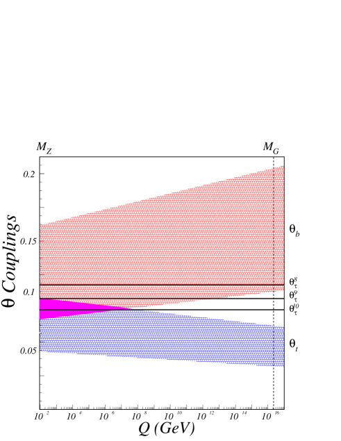
Figure 2: Renormalization scale evolution of the coefficients $\theta_{t}$, $\theta_{b}$ and $\theta_{\tau}^{8,9,10}$ couplings and their uncertainities according to the SM RGE equations. The three coefficients and their uncertainities shown in the plot were calculated using Eqs. 19, 20 and 24-26. The ligther quark masses used were extracted using sum rules.

In the case of the SM and the MSSM these effects can be calculated approximately from available one-loop renormalization group equations Babu:1992qn . For the Standard Model we obtain $\xi_{b}=\xi_{t}^{-1}=\xi$ and $\xi$ is defined by,

$$\xi\approx{\rm Exp}\left[\frac{3}{32\pi^{2}}\ln\left(\frac{\mu}{\mu_{0}}\right)\left(1-\left(\frac{m_{b}}{m_{t}}\right)^{2}\right)\right],$$ (31)

since $m_{b}/m_{t}\approx 2\times 10^{-2}$ this is approximately,

$$\xi\approx\left(\frac{\mu}{\mu_{0}}\right)^{\frac{3}{32\pi^{2}}}.$$ (32)

Moreover the tau lepton Yukawa renormalization factor is very small,

$$\xi_{\tau}\approx{\xi}^{\left(\frac{m_{\tau}}{m_{t}}\right)^{2}}\approx\left(\frac{\mu}{\mu_{0}}\right)^{-\left(\frac{3}{32\pi^{2}10^{4}}\right)}.$$ (33)

We are interested in evaluating how the correlations found in Sec. II evolve with the renormalization scale when including Yukawa corrections. To this end let us define the dimensionless ratios,

$$\theta_{b}=\left[\frac{m^{3}_{s}}{m_{b}^{2}m_{d}}\right]^{\frac{1}{2}},\quad\theta_{t}=\left[\frac{m^{3}_{c}}{m_{t}^{2}m_{u}}\right]^{\frac{1}{2}},\quad\theta_{\tau}=\frac{1}{9}\left[\frac{m^{3}_{\mu}}{m_{\tau}^{2}m_{e}}\right]^{\frac{1}{2}},$$ (34)

Their evolution, using Eqs. 28, 29 and 30, is given by,

$$\left(\frac{\theta_{b}}{\theta_{t}}\right)_{\mu}\approx\left(\frac{\theta_{b}}{\theta_{t}}\right)_{\mu_{0}}\xi^{2},\quad\left(\frac{\theta_{b}}{\theta_{\tau}}\right)_{\mu}\approx\left(\frac{\theta_{b}}{\theta_{\tau}}\right)_{\mu_{0}}\xi.$$ (35)

If we assume that $\mu/\mu_{0}=M_{G}/M_{Z}\approx 10^{14}$ we obtain $\xi\approx 1.36$. If we extrapolate the mass relations up to the GUT scale using SM RGEs we obtain,

$$\left(\frac{\theta_{b}}{\theta_{t}}\right)_{M_{G}}\approx 2.8\pm 1.0,$$ (36)

and

$$\left(\frac{\theta_{b}}{\theta_{\tau}}\right)_{M_{G}}\approx 3.5\pm 2.6,$$ (37)

which must be compared with the low energy ratios calculated in Sec. II

$$\left(\frac{\theta_{b}}{\theta_{t}}\right)_{M_{Z}}=1.5\pm 1.0,$$ (38)

and

$$\left(\frac{\theta_{b}}{\theta_{\tau}}\right)_{M_{Z}}=7.5\pm 2.6.$$ (39)

Therefore the renormalization up to the GUT scale seems to spoil the mass correlation between the up and down-type quark sector. These results are summarized in Fig. 2 and they may indicate that the Yukawa scale, the scale where the Yukawa couplings are generated, is an intermediate scale much lower than the GUT scale or alternatively that is not correct to use SM RGEs in the evolution of the fermion masses up to the GUT scale. If we assume that the couplings evolve according to the MSSM RGEs the results depend on $\tan\beta$, the ratio of Higgs expectation values in the MSSM. We obtain,

$$\xi_{b} \approx \xi_{t}^{1/3}\approx{\rm Exp}\left[-\frac{1}{16\pi^{2}}\ln\left(\frac{\mu}{\mu_{0}}\right)\right],~{}t_{\beta}\simeq 1,$$ (40)

$$\xi_{b} \approx \xi_{t}\approx{\rm Exp}\left[-\frac{1}{4\pi^{2}}\ln\left(\frac{\mu}{\mu_{0}}\right)\right],~{}t_{\beta}\gg 1.$$ (41)

Therefore we obtain the following scaling factors for low $\tan\beta$,

$$\left(\frac{\theta_{b}}{\theta_{t}}\right)_{\mu} \approx \left(\frac{\theta_{b}}{\theta_{t}}\right)_{\mu_{0}}\xi^{4/3},$$ (42)

$$\left(\frac{\theta_{b}}{\theta_{\tau}}\right)_{\mu} \approx \left(\frac{\theta_{b}}{\theta_{\tau}}\right)_{\mu_{0}}\xi^{-2/3}.$$ (43)

Here $\xi$ was defined in Eq. 32 and using $\mu/\mu_{0}=M_{G}/M_{Z}$ we obtain $\xi^{4/3}\approx 1.5$ and $\xi^{-2/3}\approx 0.81$. For large $t_{\beta}$ we obtain,

$$\left(\frac{\theta_{b}}{\theta_{t}}\right)_{\mu} \approx \left(\frac{\theta_{b}}{\theta_{t}}\right)_{\mu_{0}},$$ (44)

$$\left(\frac{\theta_{b}}{\theta_{\tau}}\right)_{\mu} \approx \left(\frac{\theta_{b}}{\theta_{\tau}}\right)_{\mu_{0}}\xi^{-8/3}.$$ (45)

Here $\xi^{-8/3}\approx 0.44$ for $\mu/\mu_{0}=M_{G}/M_{Z}$. Therefore in the MSSM, for both cases low and large $\tan\beta$, we cannot extrapolate the mass relations to scales as high as the GUT scale without spoiling the successful low energy mass relations. This again may be an indication that the Yukawa scale is not so far from the electroweak scale. We would like to point out that the ratios of first to second generation fermion masses; $m_{d}/m_{s}$, $m_{u}/m_{c}$ and $m_{e}/m_{\mu}$, receive tiny Yukawa renormalization factors. Therefore the mass relation,

$$\left[\frac{m_{d}}{m_{s}}\right]^{1/2}=\left[\frac{m_{u}}{m_{c}}\right]^{1/4}=3\left[\frac{m_{e}}{m_{\mu}}\right]^{1/2},$$ (46)

can be considered renormalization scale independent. To sum up, this analysis indicates that the second empirical relation, as given by Eq. 27, may be optimal at some intermediate or low energy scale. Nevertheless, the present uncertainities in the ligther quark masses are not small enough to allow us the determination of the scale at which this empirical formula is optimal.

IV The fermion mass hierarchies

The empirical formulas found in the previous section can be simply understood if the fermion mass hierarchies are expressed as a function of two real parameters that we will denote hereafter by $\theta$ and $\lambda$. Let us assume that the ratios of running masses can be written in the following form,

$$\left(m_{d},m_{s}\right) = \left(\theta\lambda^{3},\theta\lambda\right)m_{b},$$ (47)

$$\left(m_{u},m_{c}\right) = \left(\theta\lambda^{6},\theta\lambda^{2}\right)m_{t},$$ (48)

$$\left(m_{e},m_{\mu}\right) = \left(\frac{1}{3}\theta\lambda^{3},3\,\theta\lambda\right)m_{\tau},$$ (49)

We can easily prove that if this is the case we obtain immediately the correct empirical mass relations,

$$\lambda = \left[\frac{m_{d}}{m_{s}}\right]^{1/2}=\left[\frac{m_{u}}{m_{c}}\right]^{1/4}=3\left[\frac{m_{e}}{m_{\mu}}\right]^{1/2}$$ (50)

$$\theta = \left[\frac{m_{s}^{3}}{m_{b}^{2}m_{d}}\right]^{1/2}=\left[\frac{m_{c}^{3}}{m_{t}^{2}m_{u}}\right]^{1/2}=\frac{1}{9}\left[\frac{m_{\mu}^{3}}{m_{\tau}^{2}m_{e}}\right]^{1/2}.$$ (51)

In other words we can say the the hierarchies in Eqs. 47–49 solve the Eqs. 50–51. We pointed out before that $\lambda$ corresponds approximately to the Cabibbo angle. The parameter $\theta$ may be considered a new flavor parameter that seems to suppress, in all three fermion sectors, both first and second generation masses in the same amount with respect to the third generation. The fact that $\theta$ and $\lambda$ connect different fermion sectors and that the correlations we have found work at a quantitative level suggest that $\theta$ and $\lambda$ could be directly related to the underlying theory of flavor. We expect that any theory of flavor must be able to explain these correlations from first principles, and perhaps provide a prediction for $\theta$ and $\lambda$.

Although the important uncertainties in the current extraction of lighter quark masses make impossible to know to what extent the relations in Eqs. 50 and 51 hold, it is plausible to study the implications derived of assuming that these relations are exact or almost exact. If this were the case we are lead to assume that the charged lepton sector is providing us the most precise determination of the basic flavor parameters $\lambda$ and $\theta$, $\lambda\approx 0.21$ and $\theta\approx 0.095$.

V The CKM mixing matrix hierarchies (neglecting CP-violation)

A theory of flavor must explain the fermion mass hierarchies and the measured flavor mixing. Therefore it is important for the reconstruction of the Yukawa matrices to study if it is possible to express the absolute values of the CKM matrix elements as simple functions of the two basic flavor parameters, $\theta$ and $\lambda$. We include for completeness a compilation of the latest extractions of the elements of the CKM mixing matrix, $\left|{\cal V}_{CKM}^{\hbox{exp}}\right|$,

$$\left[\begin{array}[]{ccc}0.9739\pm 0.0005&0.2224\pm 0.0036&0.00357\pm 0.00031\\ 0.2224\pm 0.0035&0.9740\pm 0.0008&0.0415\pm 0.0008\\ \leq 0.005&0.0405\pm 0.0035&0.99915\pm 0.00015\end{array}\right].$$ (52)

Here to obtain $\left|V_{ud}\right|$ two measurements, from superallowed Fermi transitions and nuclear beta decay, have been combined, as in page 36 of the 2002 CERN Workshop on the CKM matrix  Battaglia:2003in . The value used for $\left|V_{us}\right|$ was calculated in page 37 of the same reference by requiring unitarity. For $\left|V_{ub}\right|$ and $\left|V_{cb}\right|$ we use the latest extractions from B physics, as in page 6 of the same reference. For the rest of CKM elements we use the 2002 PDG compilation values Hagiwara:fs . We fit each of the measured absolute values of the CKM matrix elements to simple functions of products of integer powers of the fundamental parameters $\lambda$ and $\theta$. We use the numerical values for $\theta$ and $\lambda$ as determined from the charged lepton sector, i.e. $\theta\approx 0.095$ and $\lambda\approx 0.21$, and look for correlations of the form $r~{}\theta^{p}\lambda^{q}$, where $p$ and $q$ are integer numbers and $r$ is a low integer or rational number. We obtain as the best fits to the measured CKM elements the functions,

$$\left|V_{us}\right| = 0.2224\pm 0.0036~{}\approx\lambda$$ (53)

$$\left|\frac{V_{cb}}{V_{us}}\right| = 0.187\pm 0.006\quad~{}\approx 2\theta$$ (54)

$$\left|\frac{V_{ub}}{V_{cb}}\right| = 0.086\pm 0.009\quad~{}\approx\left(\frac{\lambda}{2},\theta\right)$$ (55)

We note that the ratio $\left|V_{ub}/V_{cb}\right|$ has an important uncertainity which, in principle, would allow us to fit it at $2\sigma$ to both terms $\theta$ or $\lambda/2$. The large experimental uncertainty in the entry $\left|V_{td}\right|$ does not allow us to implement a fit to $\theta$ and $\lambda$. Therefore we obtain, ignoring CP-violating phases, the following structure for the CKM matrix as a function of the parameters $\theta$ and $\lambda$,

$${\cal V}_{\rm CKM}(\lambda,\theta)\approx\left[\begin{array}[]{ccc}1-\lambda^{2}/2&-\lambda&a\\ \lambda&1-b^{2}&-2\theta\lambda\\ c&2\theta\lambda&1-2\theta^{2}\lambda^{2}\end{array}\right],$$ (56)

where $a$, $b$ and $c$ must be considered unknown functions of $\theta$ and $\lambda$ which can be calculated requiring the matrix ${\cal V}_{\rm CKM}(\lambda,\theta)$ to be unitary. This determines a system of three equations which can be solved requiring unitarity to order ${\cal O}(\lambda^{3})$,

$$V_{ud}V_{cd}+V_{us}V_{cs}+V_{ub}V_{cb} = {\cal O}(\lambda^{4}),$$ (57)

$$V_{ud}V_{td}+V_{us}V_{ts}+V_{ub}V_{tb} = {\cal O}(\lambda^{4}),$$ (58)

$$V_{td}V_{cd}+V_{ts}V_{cs}+V_{tb}V_{cb} = {\cal O}(\lambda^{4}).$$ (59)

We obtain $a=c=\theta\lambda^{2}$ and $b=\lambda^{2}/2+2\theta^{2}\lambda^{2}$. Therefore we obtain for $\left|{\cal V}_{\rm CKM}(\lambda,\theta)\right|$,

$$\left[\begin{array}[]{ccc}1-\lambda^{2}/2&\lambda&\theta\lambda^{2}\\ \lambda&1-\lambda^{2}(1+4\theta^{2})/2&2\theta\lambda\\ \theta\lambda^{2}&2\theta\lambda&1-2\theta^{2}\lambda^{2}\end{array}\right],$$ (60)

We note that if we had chosen the correlation $\left|V_{ub}/V_{cb}\right|\approx\theta$ instead of $\left|V_{ub}/V_{cb}\right|\approx\lambda/2$ the CKM matrix could not meet the unitarity requirement.

We also note that one of the most interesting characteristics of the Yukawa matrices proposed in this section is that they account for the quark mass ratios and CKM elements quantitatively with only two real parameters. It is known that a general unitary matrix can be parametrized using three mixing angles and a complex phase. Our results indicate that only two real parameters seem to be necessary to account quite well for the absolute values of the CKM elements and quark mass ratios. The CKM reconstructed matrix in Eq. 60 can be expressed, using the standard PDG notation Hagiwara:fs as the product of three rotation matrices, each around a different axis,

$$\left|{\cal V}_{\rm CKM}\right|\approx R^{12}(\theta_{12})R^{23}(\theta_{23})R^{13}(\theta_{13}).$$ (61)

where $\theta_{12}=\lambda$, $\theta_{23}=\theta\lambda$ and $\theta_{13}=\theta\lambda^{2}$. Here $R^{12}(\theta_{12})$ is a rotation of angle $\lambda$ in the first-second generation plane,

$$R^{12}(\lambda)\approx\left[\begin{array}[]{ccc}1-\frac{\lambda^{2}}{2}&-\lambda&0\\ \lambda&1-\frac{\lambda^{2}}{2}&0\\ 0&0&1\end{array}\right],$$ (62)

and $R^{23}(\theta_{23})$ and $R^{13}(\theta_{13})$ are a rotations of angle $\theta\lambda$ and $\theta\lambda^{2}$ around the second-third and first-third generation planes respectively,

$$R^{23}(2\theta\lambda)\approx\left[\begin{array}[]{ccc}1&0&0\\ 0&1-2\theta^{2}\lambda^{2}&-2\theta\lambda\\ 0&2\theta\lambda&1-2\theta^{2}\lambda^{2}\end{array}\right],$$ (63)

and,

$$R^{13}(\theta\lambda^{2})\approx\left[\begin{array}[]{ccc}1-\frac{\theta^{2}\lambda^{4}}{2}&0&-\theta\lambda^{2}\\ 0&1&0\\ \theta\lambda^{2}&0&1-\frac{\theta^{2}\lambda^{4}}{2}\end{array}\right].$$ (64)

We have seen that present experimental data allow us to express the fermion mass hierarchies and the absolute values of the CKM matrix elements as a function of two basic parameters $\theta$ and $\lambda$. Throughout this section we have ignored the presence of a CP-violating phase, which is required experimentally. The presence of CP-violating phases could affect seriously the relations between the absolute values of some of the CKM elements and the parameters $\lambda$ and $\theta$ as proposed in this section. We will see in Sec. VII that CP-violating phases can be included in the previous analysis giving an excellent fit to the data. In the next section we will show that to leading order in $\lambda$ there is a unique set of Yukawa matrices that can reproduce these hierarchies.

VI Quark Yukawa matrices (neglecting CP-violation)

In this section we propose a particular reconstruction of the quark Yukawa matrices that can explain the quark mass and mixing hierarchies found in previous sections. We restrict our discussion to symmetric mass matrices. We will also assume that correct CKM elements or masses do not arise as approximate cancellations requiring the tuning of different Yukawa matrix elements. It is convenient to define the $3\times 3$ normalized fermion mass matrices as,

$$\widehat{\bf m}_{D}=\frac{1}{\widehat{m}_{b}}{\bf m}_{D},\quad\widehat{\bf m}_{U}=\frac{1}{\widehat{m}_{t}}{\bf m}_{U}.$$

Here ${\bf m}_{D,U}$ are the quark mass matrices and $\widehat{m_{b}}$ and $\widehat{m_{t}}$ are normalized bottom and top quark masses, which are defined as the ratio of bottom and top quark running masses over the largest eigenvalue of the respective normalized matrix. We have the freedom to choose the entry (33) in the normalized mass matrices equal to 1, which correspond to the heaviest eigenvalue. Although not diagonal in the gauge basis the matrix ${\bf m}_{D}$ can be brought to diagonal form in the mass basis by a biunitary diagonalization, $({\cal V}^{d}_{L})^{\dagger}{\bf m}_{D}{\cal V}^{d}_{R}=\left(m_{d},m_{s},m_{b}\right)$. Analogously the up-type quark mass matrix, ${\bf m}_{U}$, can be brought to diagonal form in the mass basis by a biunitary diagonalization, $({\cal V}^{u}_{L})^{\dagger}{\bf m}_{U}{\cal V}^{u}_{R}=\left(m_{u},m_{c},m_{t}\right)$. The CKM mixing matrix is defined by ${\cal V}_{CKM}={\cal V}^{u\dagger}_{L}{\cal V}^{d}_{L}$.

First we note that it is not possible to generate the Cabibbo angle, $\lambda\approx\left|V_{us}\right|$, from the mixing between the first and second generations in the up–type quark sector. The normalized charm quark mass is approximately $\theta\lambda^{2}$, therefore to generate the correct magnitude for $\left|V_{us}\right|$ from $\left|{\cal V}^{u}_{L}\right|_{21}$, $\left|{\cal V}^{u}_{L}\right|_{21}\approx(\widehat{\bf m}_{U})_{12}/(\widehat{\bf m}_{U})_{22}$, we would need $(\widehat{\bf m}_{U})_{12}\approx\theta\lambda^{3}$ but if it this were the case the normalized up mass would be too heavy, $m_{u}/m_{t}\approx(\widehat{\bf m}_{U})_{12}^{2}/(\widehat{\bf m}_{U})_{22}\approx\theta\lambda^{4}$, which is in disagreement with the measured up-top mass hierarchy, $m_{u}/m_{t}\approx\theta\lambda^{6}$. Obtaining the correct up-quark mass give us a bound on the entries of the upper-left submatrix of the normalized up-type quark matrix, which must look like,

$$(\widehat{\bf m}_{U})_{2\times 2}^{\rm u-c}=\left[\begin{array}[]{ccc}\leq{\cal O}(\theta\lambda^{6})&\leq{\cal O}(\theta\lambda^{4})\\ \leq{\cal O}(\theta\lambda^{4})&\theta\lambda^{2}\end{array}\right].$$ (65)

Therefore the Cabibbo angle must arise from first–second generation mixing in the down-type quark sector. We pointed out in the previous sections that the measured hierarchies in the down-type quark sector can be written as,

$$\frac{m_{d}}{m_{b}}\approx\theta\lambda^{3}<<\frac{m_{s}}{m_{b}}\approx\theta\lambda<\left|V_{us}\right|\approx\lambda.$$ (66)

We note that assuming $(\widehat{\bf m}_{D})_{12}=\theta\lambda^{2}$ and $(\widehat{\bf m}_{D})_{22}=\theta\lambda\approx m_{s}/m_{b}$, we obtain $(\widehat{\bf m}_{D})_{12}^{2}/(\widehat{\bf m}_{D})_{22}=\theta\lambda^{3}\approx m_{d}/m_{b}$ and $(\widehat{\bf m}_{D})_{12}/(\widehat{\bf m}_{D})_{22}=\lambda$. This is consistent with a down quark mass mainly generated from the first–second generation mixing as first pointed out by discrete , i.e.,

$$\left(\widehat{\bf m}_{D}\right)_{2\times 2}^{d-s}=\left[\begin{array}[]{cc}0&\theta\lambda^{2}\\ \theta\lambda^{2}&\theta\lambda\end{array}\right],$$ (67)

since in this case one correctly obtains $\left|{\cal V}_{L}^{d}\right|_{12}\approx(\widehat{\bf m}_{D})_{12}/(\widehat{\bf m}_{D})_{22}=\lambda\approx\left|V_{us}\right|$. Furthermore, as shown in the previous section, the measured hierarchies between the CKM elements can be written as,

$$\left|V_{ub}\right|\approx\theta\lambda^{2}<\left|V_{cb}\right|\approx 2\theta\lambda\simeq(m_{s}/m_{b})\approx\theta\lambda<\left|V_{us}\right|\approx\lambda.$$ (68)

We note that if we additionally assume that $(\widehat{\bf m}_{D})_{23}=2\theta\lambda$ then we obtain the correct $\left|V_{cb}\right|$, since $\left|{\cal V}_{L}^{d}\right|_{23}=(\widehat{\bf m}_{D})_{23}/(\widehat{\bf m}_{D})_{33}=2\theta\lambda$. One can wonder if it would be possible to fully generate the CKM matrix entry $\left|V_{ub}\right|$ from the (23)-(12) mixing in the down-type quark sector, or in other words, if we can assume that the normalized down-type quark matrix has a zero in the entry (13) and (31). A calculation of the diagonalization matrices show us that this possibility is not viable. It this were the case $\left|{\cal V}_{L}^{d}\right|$ would be given by, $\left|{\cal V}_{L}^{d}\right|\approx\theta^{2}\lambda^{3}$ which is two orders of magnitude below the measured value for $\left|{\cal V}_{cb}\right|$, $\left|{\cal V}_{cb}\right|\approx\theta\lambda^{2}$. Therefore we need to generate $\left|{\cal V}_{cb}\right|$ directly from a non-zero $(\widehat{\bf m}_{D})_{13}$ entry,

$$\widehat{\bf m}_{D}=\left[\begin{array}[]{ccc}0&\theta\lambda^{2}&\theta\lambda^{2}\\ \theta\lambda^{2}&\theta\lambda&2\theta\lambda\\ \theta\lambda^{2}&2\theta\lambda&1\end{array}\right].$$ (69)

We must note here that the possibility to fully generate $\left|V_{ub}\right|$ in the up-sector is not viable, if that were the case we would generate a up-quark mass one order of magnitude too heavy. This $\widehat{\bf m}_{D}$ matrix would predict successfully all the elements of the CKM mixing matrix, assuming the mixing in the up-type sector does not affect the leading order predictions in $\lambda$. This can be observed in the expressions for the diagonalization matrix, ${\cal V}_{L}^{d}$, given by,

$${\cal V}_{L}^{d}=\left[\begin{array}[]{ccc}1-\frac{\lambda^{2}}{2}&\lambda&-\theta\lambda^{2}\\ -\lambda&1-\frac{\lambda^{2}}{2}(1+4\theta^{2})&-2\theta\lambda\\ -\theta\lambda^{2}&2\theta\lambda&1-2\theta^{2}\lambda^{2}\end{array}\right],$$ (70)

Using this we obtain for the mass eigenvalues to leading order in $\lambda$,

$$({\cal V}^{d}_{L})^{\dagger}\widehat{\bf m}_{D}{\cal V}^{d}_{R}\approx\left(\theta\lambda^{3},\theta\lambda,1+\theta^{2}\lambda^{2}\right).$$ (71)

which is in perfect agreement with the reconstructed quark mass hierarchies in Eq. 47. In the previous reasoning we assumed that the possible flavor mixing in the up-type quark sector does not affect to leading order the predictions for the CKM matrix which are generated in the down-type sector. If this were the case, there are two simple solutions which allow us to generate the correct up-quark mass: directly from an entry (11),

$$\widehat{\bf m}_{U}=\left[\begin{array}[]{ccc}\theta\lambda^{6}&0&0\\ 0&\theta\lambda^{2}&0\\ 0&0&1\end{array}\right],$$ (72)

or from the first-second generation mixing,

$$\widehat{\bf m}_{U}=\left[\begin{array}[]{ccc}0&\theta\lambda^{4}&0\\ \theta\lambda^{4}&\theta\lambda^{2}&0\\ 0&0&1\end{array}\right],.$$ (73)

Since both possibilities make the same predictions for quark mass ratios and CKM elements both are equivalent by a rotation of the quark fields. It could be possible to generalize the previous solution to a solution that generates part of $\left|V_{cb}\right|$ from flavor mixing between second and third generations in the up-type quark sector. Let us assume that,

$$\widehat{\bf m}_{D}=\left[\begin{array}[]{ccc}0&\theta\lambda^{2}&\theta\lambda^{2}\\ \theta\lambda^{2}&\theta\lambda&(2-\epsilon)\theta\lambda\\ \theta\lambda^{2}&(2-\epsilon)\theta\lambda&1\end{array}\right],$$ (74)

and,

$$\widehat{\bf m}_{U}=\left[\begin{array}[]{ccc}\theta\lambda^{6}&0&0\\ 0&\theta\lambda^{2}&-\epsilon\theta\lambda\\ 0&-\epsilon\theta\lambda&1\end{array}\right].$$ (75)

In this case the diagonalization matrices are respectively,

$${\cal V}_{L}^{d}=\left[\begin{array}[]{ccc}1-\frac{\lambda^{2}}{2}&-\lambda&-\theta\lambda^{2}\\ \lambda&1-\frac{\lambda^{2}}{2}(1+\eta^{2}\theta^{2})&\eta\theta\lambda\\ (\epsilon-1)\theta\lambda^{2}&\eta\theta\lambda&1-\frac{1}{2}\eta^{2}\theta^{2}\lambda^{2}\end{array}\right],$$ (76)

where $\eta=(2-\epsilon)$ and,

$${\cal V}_{L}^{u}=\left[\begin{array}[]{ccc}1&0&0\\ 0&1-\epsilon^{2}\frac{\theta^{2}\lambda^{2}}{2}&-\epsilon\theta\lambda\\ 0&\epsilon\theta\lambda&1-\epsilon^{2}\frac{\theta^{2}\lambda^{2}}{2}\end{array}\right].$$ (77)

These two solutions; the one given by Eqs. 69 and 72-73 or the one given by Eqs. 74 and 75 are indistinguishable in their predictions for quark mass ratios and CKM elements to first order in powers of $\lambda$. Both reproduce the correct form for the CKM matrix in Eq. 60. Therefore they are equivalent and can be related by a rotation of the quark fields. We note that from their diagonalization we obtain the correct empirical expressions for $\lambda$ and $\theta$ as a function of dimensionless quark mass ratios (see Eqs. 18 & 27). To first order,

$$\lambda \approx \left(\frac{m_{d}}{m_{s}}\right)^{\frac{1}{2}}\approx\left(\frac{m_{u}}{m_{c}}\right)^{\frac{1}{4}},$$ (78)

$$\theta \approx \left(\frac{m_{s}^{3}}{m_{b}^{2}m_{d}}\right)^{\frac{1}{2}}\approx\left(\frac{m_{u}^{3}}{m_{c}^{2}m_{t}}\right)^{\frac{1}{2}},$$ (79)

Nevertheless, there are in principle other solutions that are not equivalent to the family of solutions here proposed and make the same predictions to leading order. These could be differentiated in their precision predictions for mass ratios and CKM elements when including higher orders in powers of $\lambda$.

VII Introducing CP-violation

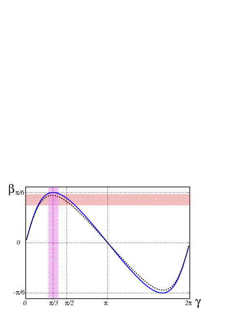
Figure 3: Relation between CP-violating phases $\beta$ and $\gamma$ as predicted by the quark Yukawa matrices in Eqs. 72 and 81. The horizontal hatched strip corresponds to the measurement $\sin(2\beta)_{\rm exp}=0.78\pm 0.08$. The vertical hatched strip corresponds to the 1$\sigma$ global fit for the angle $\gamma$, $\gamma_{\rm fit}=61^{\circ}\pm 11^{\circ}$. The solid curve corresponds to the leading order relation between $\beta$ and $\gamma$ given by Eq. 85. The dotted curved corresponds to the next to leading order relation given by Eq. 104

We have seen in the previous section that a set of two parameter Yukawa matrices of the form given in Eqs. 69 and 72 represents a family of solutions, in the basis where the up-type Yukawa matrix is diagonal, that can account for the quark mass ratios and the absolute values of the CKM matrix elements. It is possible to introduce complex phases in this picture to account for the measured CP-violation without spoiling these successful predictions. In order to do so we promote the real symmetric matrix in Eq. 69 to be hermitian. In the most general hermitian case we can introduce complex phases in the form,

$$\widehat{\bf m}_{D}=\left[\begin{array}[]{ccc}0&e^{i\psi_{1}}\theta\lambda^{2}&e^{i\psi_{2}}\theta\lambda^{2}\\ e^{-i\psi_{1}}\theta\lambda^{2}&\theta\lambda&2e^{i\psi_{3}}\theta\lambda\\ e^{-i\psi_{2}}\theta\lambda^{2}&2e^{-i\psi_{3}}\theta\lambda&1\end{array}\right].$$ (80)

By a redefinition of the phases of the quark fields this can be simplified to,

$$\widehat{\bf m}_{D}=\left[\begin{array}[]{ccc}0&\theta\lambda^{2}&e^{-i\gamma}\theta\lambda^{2}\\ \theta\lambda^{2}&\theta\lambda&2\theta\lambda\\ e^{i\gamma}\theta\lambda^{2}&2\theta\lambda&1\end{array}\right].$$ (81)

where $\gamma=-(\psi_{2}-\psi_{1}-\psi_{3})$. If this were the case we obtain for the CKM matrix, ${\cal V}_{CKM}={\cal V}_{L}^{d}$, to leading order in $\lambda$,

$$\left[\begin{array}[]{ccc}1-\frac{\lambda^{2}}{2}&\lambda&-e^{-i\gamma}\theta\lambda^{2}\\ -\lambda&1-\frac{\lambda^{2}}{2}(1+4\theta^{2})&-2\theta\lambda\\ (e^{i\gamma}-2)\theta\lambda^{2}&2\theta\lambda&1-2\theta^{2}\lambda^{2}\end{array}\right].$$ (82)

The angle $\gamma$ introduced this way coincides with the standard definition,

$$\gamma={\rm Arg}\left[-\frac{V_{ud}V^{*}_{ub}}{V_{cd}V^{*}_{cb}}\right],$$ (83)

Furthermore the angle $\beta$ is given by,

$$\beta={\rm Arg}\left[-\frac{V_{cd}V^{*}_{cb}}{V_{td}V^{*}_{tb}}\right].$$ (84)

The angle $\alpha$ can be obtained from the relation, $\alpha+\beta+\gamma=180^{\circ}$. The hermitian matrix of the form given by Eq. 81 predicts a simple relation between the angles $\beta$ and $\gamma$, which to leading order is,

$$\beta={\rm Arg}\left[2-e^{-i\gamma}\right]$$ (85)

The angle $\beta$ can been determined with $7\%$ accuracy using the experimental determination of $\sin 2\beta$, $\sin 2\beta=0.78\pm 0.08$. We obtain $\beta_{\rm exp}=25.7^{\circ}\pm 3.5^{\circ}$. This indicates that the value of $\beta$ that nature has chosen is close to the maximum value that $\beta$ can reach in the case under consideration, $\beta_{\rm max}=30^{\circ}$, which appears for $\gamma=60^{\circ}$,

$$\frac{{\rm d}\beta}{{\rm d}\gamma}=0\rightarrow\gamma=60^{\circ}\rightarrow\alpha=90^{\circ}.$$ (86)

We note that this does not correspond with the case of maximal CP-violation. If we compute the determinant of Jarlskog matrix, ${\cal C}=\left[\widehat{\bf m}_{U}\widehat{\bf m}_{U}^{\dagger},\widehat{\bf m}_{D}\widehat{\bf m}_{D}^{\dagger}\right]$, we obtain,

$${\rm det}~{}{\cal C}=2{\cal J}\theta^{4}\lambda^{6}+{\cal O}(\lambda^{11}),$$ (87)

where ${\cal J}$ is the Jarlskog parameter, the invariant measure of CP-violation, which in our case is given by,

$${\cal J}=2\sin(\gamma)\theta^{2}\lambda^{4}\left(1+{\cal O}(\theta\lambda)\right).$$ (88)

We note that the maximal CP-violation case corresponds to $\gamma=\pi/2$ and using the Eq. 85 this corresponds to,

$$\frac{{\rm d}{\cal J}}{{\rm d}\gamma}=0\rightarrow\gamma=90^{\circ}\rightarrow\beta=26.6^{\circ}.$$ (89)

Although there is a simple relation, see Eq. 85, between $\beta$ and $\gamma$ the angle $\gamma$, as can be seen in figure 3, cannot be determined with good precision from that relation and the experimentally determined value of $\beta$. We obtain, $\gamma_{\rm theo}=65^{\circ}\pm 38^{\circ}$, which is in agreement with the 2004 winter global fit of the CKM elements. obtained using the results of program CKMFitter Hocker:2001xe ,

$$\gamma_{\rm exp}=61^{\circ}\pm 11^{\circ}\\$$ (90)

Alternatively we can use this experimental value of $\gamma$ to predict $\beta$ from the Eq. 85, as can be seen on Fig. 3. We obtain to leading order,

$$\beta_{\rm theo}=29.4^{\circ}\pm 0.05^{\circ}\\$$ (91)

which corresponds to $\sin(2\beta)_{\rm theo}=0.855\pm 0.001$. The Jarlskog parameter is determined experimentally to be ${\cal J}=(3.0\pm 0.3)\times 10^{-5}$. The use of the Jarlskog parameter does not allow us to extract $\gamma$ with better precision because of the uncertainties in the determination of $\lambda$ and $\theta$. On the other hand our expression for ${\cal J}$ predicts an interesting relation between ${\cal J}$ and the quark masses,

$${\cal J}\approx 2\frac{m_{d}m_{s}}{m_{b}^{2}}\sin(\gamma)\left(1+{\cal O}(\theta\lambda)\right).$$ (92)

Finally, we note that there two non-trivial characteristics in the relation between $\beta$ and $\gamma$, Eq. 85, as predicted by the CKM matrix in Eq. 82: first there is no dependence on $\lambda$ or $\theta$ to first order and second and most important the relation agrees with the experimental measurements of $\beta$ and $\gamma$.

VIII Predictions for masses and mixings

In this section we want to show that the simple three parametric Yukawa matrices proposed in Sec. VII can fit all the experimental data on the fermion spectra with precision. We study in this section precision predictions for the lighter quark masses and CKM elements. Let us assume that the $\widehat{\bf m}_{D}$ Yukawa matrix is given by Eq. 81 while the $\widehat{\bf m}_{U}$ matrix is given by Eq. 72. If we postulate these up– and down–type quark Yukawa matrices we can express the CKM elements and the quark mass ratios as a function of $\theta$, $\lambda$ and $\gamma$. The down-type quark mass ratios can be calculated to the next to leading order in $\lambda$ from the diagonalization of Eq.81,

$$\frac{m_{d}}{m_{s}} = \lambda^{2}(1-\theta\lambda(4c_{\gamma}-9)),$$ (93)

$$\frac{m_{s}}{m_{b}} = \theta\lambda(1-4\theta\lambda+\lambda^{2}).$$ (94)

Here $c_{\gamma}=\cos(\gamma)$. The up-type quark mass ratios are given by,

$$\frac{m_{u}}{m_{c}}=\lambda^{4},\quad\frac{m_{c}}{m_{t}}=\theta\lambda^{2}$$ (95)

while the absolute values of CKM matrix elements to the next to leading order in $\lambda$ are given by,

$$\left|V_{us}\right| = \lambda-2(c_{\gamma}-2)\theta\lambda^{2}+{\cal O}(\lambda^{3}),$$ (96)

$$\left|V_{ud}\right| = 1-\frac{1}{2}\lambda^{2}+2(c_{\gamma}-2)\theta\lambda^{3},$$ (97)

$$\left|V_{ub}\right| = \theta\lambda^{2}+2c_{\gamma}\theta^{2}\lambda^{3},$$ (98)

$$\left|V_{cs}\right| = 1-\frac{1}{2}\lambda^{2}(1+4\theta^{2})+2\theta\lambda^{3}(c_{\gamma}-2),$$ (99)

$$\left|V_{cb}\right| = 2\theta\lambda(1+\theta\lambda),$$ (100)

$$\left|V_{td}\right| = (5-4c_{\gamma})^{\frac{1}{2}}\left(\theta\lambda^{2}+4\theta^{2}\lambda^{3}\right),$$ (101)

$$\left|V_{ts}\right| = 2\theta\lambda+2\theta^{2}\lambda^{2}+(c_{\gamma}-1)\theta\lambda^{3},$$ (102)

$$\left|V_{tb}\right| = 1-2\lambda^{2}\theta^{2}-4\theta^{3}\lambda^{3}.$$ (103)

and $\left|V_{cd}\right|=\left|V_{us}\right|$.

experimental input parameters
$\left|V_{us}\right|$	$0.2225\pm 0.0035$
$m_{c}/m_{t}$	$(3.7\pm 0.4)\times 10^{-3}$
$\gamma$	$61^{\circ}\pm 11^{\circ}$
$m_{t}^{\rm pole}$	$174.3\pm 5.1~{}{\rm GeV}$
$m_{b}(m_{b})_{\overline{\rm MS}}$	$4.2\pm 0.1~{}{\rm GeV}$
$m_{\tau}^{\rm pole}$	$1.7769\pm 0.0003~{}{\rm GeV}$
predictions
$\lambda$	$0.211\pm 0.007$
$\theta$	$0.083\pm 0.014$
$\sin(2\beta)$	$0.824\pm 0.004$
$\left|V_{ud}\right|$	$0.975\pm 0.002$
$\left|V_{ub}\right|$	$0.0037\pm 0.0009$
$\left|V_{cs}\right|$	$0.9771\pm 0.0017$
$\left|V_{cb}\right|$	$0.035\pm 0.007$
$\left|V_{td}\right|$	$0.007\pm 0.002$
$\left|V_{ts}\right|$	$0.035\pm 0.007$
$\left|V_{tb}\right|$	$0.9993\pm 0.0002$
$m_{u}(2~{}{\rm GeV})_{\overline{\rm MS}}$	$2.1\pm 0.9$ MeV
$m_{d}(2~{}{\rm GeV})_{\overline{\rm MS}}$	$4.2\pm 1.4$ MeV
$m_{s}(2~{}{\rm GeV})_{\overline{\rm MS}}$	$84\pm 19$ MeV
$m_{e}^{\rm pole}$	$0.49\pm 0.13~{}{\rm MeV}$
$m_{\mu}^{\rm pole}$	$92\pm 17~{}{\rm MeV}$

Table 2: Low energy measured values of $\left|V_{us}\right|$, the ratio of running masses $m_{c}/m_{t}$ and the $1~{}\sigma$ global fit of the phase $\gamma$ are used to determine $\lambda$ and $\theta$ from Eqs. 95 & 96. Then these are used to predict the three lighter quark masses, $\sin(2\beta)$, the rest of CKM matrix elements and the muon and electron masses from the Yukawa matrices in Eqs. 72 , 81 and 106.

while $\beta$ and $\gamma$ are related to the next order in $\lambda$ by,

$$\beta={\rm Arg}\left[(2-e^{-i\gamma})\left(1+\theta\lambda(1-2e^{i\gamma})\right)\right].$$ (104)

We use as an input three parameters determined experimentally: $\left|V_{us}\right|$, $m_{c}/m_{t}$ and the angle $\gamma$, whose numerical values can be read in table 2. We determine $\lambda$, $\theta$ solving numerically the system of Eqs. 95 and 96. Finally we use these together with the measured third generation fermion masses to predict the masses of the lighter quarks, the rest of the CKM elements and $\sin(2\beta)$, the results are shown in table 2. It is remarkable that all the next to leading order predictions agree with the respective measured values. We note that the value predicted for $\sin(2\beta)$ is slightly lower than the value predicted to leading order in the previous section.

It is worth to note that a theory of flavor must predict succesfully the so-called $Q$ factor. This is a combination of quark masses which has been determined experimentally from pseudoscalar meson masses to a $3.5$ % accuracy. It is defined by,

$$Q=\frac{\frac{m_{s}}{m_{d}}}{\sqrt{1-\left(\frac{m_{u}}{m_{d}}\right)^{2}}}=22.7\pm 0.08.$$ (105)

In our case using the central values for $\theta$, $m_{t}$, $m_{b}$ and $\gamma$ in table 2 and $\lambda=0.211\pm 0.007$ we obtain $Q=23.5\pm 0.80$ which agrees at 1$\sigma$ with the experimental result. For $\lambda=0.218$ we obtain the central value $Q=22.7$. We note that it is not convenient to use the measured value of Q to determine one of the basic parameters, instead of $\left|V_{us}\right|$ or $m_{c}/m_{t}$, because Q contains a implicit dependence on the uncertainity in the top and bottom quark masses.

To sum up, there are six input parameters in the up, down and charged lepton Yukawa matrices: $\theta$, $\lambda$, $\gamma$, $m_{b}(m_{b})$, $m_{t}^{\rm pole}$ and $m_{\tau}^{\rm pole}$. We can choose two observables to determine $\theta$ and $\lambda$. In table 2 we chose $\left|V_{us}\right|$ and the charm/top quark mass ratio. Therefore we obtain the following true predictions: two quark mixing angles, a prediction for the CP-phase $\beta$, the up, down and strange quark masses plus the electron and muon masses. A total of 8 true succesfull predictions as can be seen in table II.

IX Charged lepton sector spectra and the Georgi-Jarlskog factor

We pointed out in Sec. II, see Eqs. 18 and 27, that there are empirical relations that connect the charged lepton and the quark masses. In this section we argue that there is already a simple explanation for these relations, the Georgi-Jarlskog factor. Let us assume that the normalized Yukawa matrix for the charged lepton sector is given by,

$$\widehat{\bf m}_{L}=\left(\begin{array}[]{ccc}0&\theta\lambda^{2}&e^{-i\gamma}\theta\lambda^{2}\\ \theta\lambda^{2}&{\bf 3}~{}\theta\lambda&2\theta\lambda\\ e^{i\gamma}\theta\lambda^{2}&2\theta\lambda&1\end{array}\right).$$ (106)

If this were the case the charged lepton mass ratios could be calculated by a biunitary diagonalization,

$$\frac{m_{e}}{m_{\mu}} = \frac{1}{9}\lambda^{2}(1-4\theta\lambda(\cos\gamma-\frac{17}{12})),$$ (107)

$$\frac{m_{\mu}}{m_{\tau}} = 3\theta\lambda(1-\frac{4}{3}\theta\lambda+\frac{1}{9}\lambda^{2}).$$ (108)

which would explain the observed empirical formulas. A matrix like Eq. 106, especially the relation $(\widehat{\bf m}_{L})_{22}=3(\widehat{\bf m}_{D})_{22}$, could be understood in the context of grand unified models. For instance, by embedding the quark and lepton fields in the representations ${\bf 5}$ and ${\bf 10}$ of SU(5) and assuming a non-minimal Higgs structure in the unified theory Georgi:1979df such that the field that couples to the matter fields generating the $(\widehat{\bf m}_{L})_{22}$ entry transforms under the representation ${\bf 45}$ of SU(5). The corresponding Clebsch-Gordan factors could generate the factor 3 in the entry (22) of the charged lepton Yukawa matrix. We must emphasize that even tough the original GUT model by Georgi and Jarslkog is ruled out the Georgi-Jarslkog factor, or in other words the ${\bf 45}$ Higgs, has been used by many models especially supersymmetric GUT models which are not ruled out by current data. This may indicate that the empirical relations support a mechanism which can be implemented in many GUT models but it does not support a particular GUT model.

Using the measured charged lepton mass ratios and the 1$\sigma$ global fit value of $\gamma$ we can determine the parameters $\lambda$ and $\theta$ in the charged lepton sector from Eqs. 107 and 108. Then using the top and bottom quark masses and the results of the previous section we can predict the four lighter quark masses, the CKM elements and $\sin(2\beta)$. The results are presented in table 3. All the predictions are very close to the respective measured values, which is consistent with the numerical results in the previous section.

Alternatively one can use the values of $\lambda$ and $\theta$ as determined from the quark sector together with the measured tau lepton mass to predict the electron and muon masses from Eqs. 107 and 108. The results, which are shown in table 2, are consistent with the measured electron and muon physical masses.

input parameters
$m_{e}/m_{\mu}$	$(4.73711\pm 0.00007)\times 10^{-3}$
$m_{\mu}/m_{\tau}$	$(5.882\pm 0.001)\times 10^{-2}$
$\gamma$	$61^{\circ}\pm 11^{\circ}$
$m_{t}^{\rm pole}$	$174.3\pm 5.1~{}{\rm GeV}$
$m_{b}(m_{b})_{\overline{\rm MS}}$	$4.2\pm 0.1~{}{\rm GeV}$
predictions
$\lambda$	$0.199\pm 0.001$
$\theta$	$0.100\pm 0.001$
$\sin(2\beta)$	$0.820\pm 0.005$
$\left|V_{ud}\right|$	$0.9778\pm 0.0005$
$\left|V_{us}\right|$	$0.211\pm 0.003$
$\left|V_{ub}\right|$	$0.0040\pm 0.0001$
$\left|V_{cd}\right|$	$0.211\pm 0.003$
$\left|V_{cs}\right|$	$0.9794\pm 0.0002$
$\left|V_{cb}\right|$	$0.0405\pm 0.0006$
$\left|V_{td}\right|$	$0.0075\pm 0.0009$
$\left|V_{ts}\right|$	$0.0401\pm 0.0007$
$\left|V_{tb}\right|$	$0.99917\pm 0.00002$
$m_{c}(m_{c})_{\overline{\rm MS}}$	$1.34\pm 0.08$ GeV
$m_{u}(2~{}{\rm GeV})_{\overline{\rm MS}}$	$1.85\pm 0.17$ MeV
$m_{d}(2~{}{\rm GeV})_{\overline{\rm MS}}$	$4.2\pm 0.3$ MeV
$m_{s}(2~{}{\rm GeV})_{\overline{\rm MS}}$	$94\pm 5$ MeV

Table 3: Low energy dimensionless ratios of measured charged lepton running masses plus the $1~{}\sigma$ global fit value of the phase $\gamma$ are used to determine $\lambda$ and $\theta$ from Eqs. 107 and 108. Then these are used to predict the four lighter quark masses, $\sin(2\beta)$ and the CKM matrix elements from Eqs. 72, 81 and 104.

X Perspectives and conclusions

In this section we include some considerations regarding the possible characteristics of an underlying theory of flavor that is able to make sense of the previous results. To recapitulate,

1. There are two empirical formulas that connect the six fermion mass ratios and the CKM elements,

2. A simple three-parametric set of Yukawa matrices for the quark and charged lepton sectors can generate these relations naturally and account for the measured fermion mass ratios and CKM elements,

3. The simplest explanation of the charged lepton hierarchies requires the use of grand unification to account for the factor 3 in entry (22) of the charged lepton Yukawa matrix,

4. The proposed empirical formulas work perfectly at low energies but seem to get spoiled when extrapolated to very high energies, of the order of the GUT scale $M_{G}\approx 10^{16}$ GeV.

Additionally, the proposed Yukawa matrices have the following characteristics,

1. All the entries except entry (33) are proportional to a common parameter, $\theta$, which is approximately $\theta\approx 0.1$

2. The generation of the correct fermion mass hierarchies requires the introduction of different powers of $\lambda$, the second flavor parameter, which is approximately $\lambda\approx 0.21$

3. The CP violating phases $\beta$ and $\gamma$ are related by a simple formula, which predicts that the maximum value of $\beta$ that can be reached is close to the measured value

We note that any theory of flavor that can generate the simple set of matrices proposed in this paper (or an alternative set of matrices equivalent to leading order in $\lambda$) would automatically fit the experimental data. The generation of hierarchies in the Yukawa matrices, like the hierarchies generated by polynomial matrices in powers of $\lambda$, is relatively easy to implement through the breaking of a flavor symmetry, assuming that the vevs of the flavor breaking fields have a certain hierarchical structure. There are two characteristics I want to highlight: the presence of a common parameter in all the entries of the Yukawa matrices except entry (33), and the fact that the empirical relations seem to get spoiled when extrapolated to very high energies. A possible theory to explain the presence of a common parameter in all the entries of the Yukawa matrices except entry (33) is the radiative generation of Yukawa couplings. We note that the parameter $\theta$ has the right size to be a loop factor. If this is so, the Yukawa couplings must be generated at a scale not very high; otherwise our mass relations would be spoiled, as was pointed out above. To generate Yukawa couplings radiatively, one has to postulate the existence of additional fields belonging to two different sectors: the flavor breaking sector and the flavor messenger sector. The messenger sector fields would transmit flavor violation from the flavor breaking sector to the matter sector, generating Yukawa couplings radiatively. One more piece of the puzzle is the factor 3 in the charged lepton Yukawa matrix; the simplest explanation of this factor requires grand unification.

Interestingly, supersymmetric models can reconcile the generation of the Yukawa couplings at low energy with grand unification Ferrandis:2004ri . It is known that grand unification in the context of supersymmetric models can successfully predict the weak mixing angle if the unification scale is around $10^{16}$ GeV. This provides us with a consistent scenario where we can generate the Georgi-Jarlskog factor. On the other hand, the presence of soft supersymmetry breaking terms allows for the radiative generation of quark and charged lepton masses through sfermion–gaugino loops. The gaugino mass provides the violation of fermionic chirality required by a fermion mass, while the soft breaking terms provide the violation of chiral flavor symmetry wyler . In this case the superpartners of the Standard Model matter fields would be the flavor messengers. A supersymmetric model that implements the low energy radiative generation of Yukawa couplings has been proposed recently. This was achieved by postulating a U(2) horizontal symmetry Barbieri:1995uv that is broken by a set of supersymmetry breaking fields Ferrandis:2004ri . The model can also overcome the present constraints on supersymmetric contributions to flavor changing processes Ferrandis:2004ng .

It is known that 13 out of the 18 parameters of the Standard Model belong to the flavor sector: 9 fermion masses, 3 mixing angles and 1 CP-violating phase. We have shown in this paper that there are regularities underlying the measured fermion masses that allow us to connect them through two simple empirical formulas. This implies a reduction in the number of fundamental parameters in the underlying theory of flavor from 13 to 6. We have proposed a simple set of three-parameter Yukawa matrices, with two real parameters and a complex phase, that can precisely account for these mass relations and give us a simpler parametrization of the CKM matrix The proposed set of Yukawa matrices may make the features of the underlying theory of flavor more apparent. Any theory of flavor that is able to generate this set of matrices would automatically fit the experimental data. Furthermore, the proposed Yukawa matrices predict a simple and succesfull relation between the SM CP-violating phases. We have also pointed out that the empirical mass formulas between the quark and charged lepton masses find their simplest explanation in the context of grand unified theories. There is hope that our knowledge of the ligther quark masses is going to improve considerably in the near future by the use of lattice QCD methods. These empirical relations, if confirmed, could be a guiding light in the search for the underlying theory of flavor.

Appendix

X.1 Running Lepton masses

To compute the running charged lepton masses, I use well known expressions, included here for completeness. The physical charged lepton masses are related to the $\overline{\rm MS}$ running lepton masses, $m_{l}(\mu)_{\overline{\rm MS}}=m_{l}(\mu)$, through the relation,

$$m_{l}(\mu)=m_{l}^{\rm pole}\left(1+\Delta_{l}+\Delta_{Z}+\Delta_{W}\right)$$ (109)

where the one–loop self–energy correction is given by,

$$\Delta_{l}=\frac{\alpha(\mu)}{\pi}\left[\frac{3}{2}\ln\left(\frac{m_{l}(\mu)}{\mu}\right)-1\right],$$ (110)

and the $Z$ and $W$ boson thresholds are given by,

$$\Delta_{Z} = \frac{\alpha(\mu)}{4\pi c^{2}_{W}}\left[\left(3-6s^{2}_{W}+\frac{1}{4s^{2}_{W}}\right)\ln\left(\frac{\mu}{m_{Z}}\right)\right.$$ (111)

$$\left.+\frac{7}{4}\left(1-2s^{2}_{W}+\frac{1}{28s^{2}_{W}}\right)\right],$$

$$\Delta_{W} = \frac{\alpha(\mu)}{8\pi}\left[\ln\left(\frac{\mu}{m_{W}}\right)+\frac{1}{4}\right].$$ (112)

Using the measured physical masses,

$$m_{e}^{\rm pole} = 0.510998902\pm 0.000000021~{}\hbox{MeV},$$ (113)

$$m_{\mu}^{\rm pole} = 105.6583568\pm 0.0000052~{}\hbox{MeV},$$ (114)

$$m_{\tau}^{\rm pole} = 1776.99\pm 0.3~{}\hbox{MeV},$$ (115)

we can calculate the running masses at a common scale. We choose to evaluate the running masses at $\mu=m_{Z}$ where the self-energy correction dominates the threshold. We will use $s^{2}_{W}(m_{Z})_{\overline{\rm MS}}=0.23113(15)$, $\alpha(m_{Z})^{-1}_{\overline{\rm MS}}=127.934\pm 0.027$, $m_{W}=80.423\pm 0.039$ GeV and $m_{Z}=91.1876\pm 0.0021$ GeV. We obtain,

$$m_{e}(m_{Z}) = 0.487304\pm 0.000005~{}\hbox{MeV},$$ (116)

$$m_{\mu}(m_{Z}) = 102.8695\pm 0.0005~{}\hbox{MeV},$$ (117)

$$m_{\tau}(m_{Z}) = 1748.87\pm 0.30~{}\hbox{MeV}.$$ (118)

We note that at $Q=m_{Z}$ the larger uncertainty in the running masses comes from the uncertainty in $\alpha(m_{Z})$. These running masses were used in Sec. II to search for correlations in higher-order dimensionless ratios of charged lepton masses.

X.2 Running quark masses

To calculate the dimensionless ratios of running quark masses we must renormalize the quark masses to a common scale. For completeness we include in this section a brief explanation of the methods used to calculate running quark masses and an update of previous numerical results quarkmasses . Different quark masses are usually given at different renormalization scales. For the top quark our starting point is the pole mass. We use the CDF/DO working group average Hagiwara:fs ,

$$m_{t} = 174.3\pm 5.1~{}\hbox{GeV}.$$ (119)

For the bottom and charm quarks we start with the running masses, $m_{b}(m_{b})_{\overline{\rm MS}}$ and $m_{c}(m_{c})_{\overline{\rm MS}}$ as extracted from sum rules in Refs. bottommass & charmmass respectively. The averaged values are,

$$m_{b}(m_{b})_{\overline{\rm MS}} = 4.2\pm 0.1~{}\hbox{GeV},$$ (120)

$$m_{c}(m_{c})_{\overline{\rm MS}} = 1.28\pm 0.09~{}\hbox{GeV}.$$ (121)

This value of the charm quark mass is compatible with recent lattice calculations, $m_{c}(m_{c})_{\overline{\rm MS}}^{\rm lat}=1.26\pm 0.16~{}{\rm GeV}$  Becirevic:2001yh . For the lighter quarks we use the normalized $\overline{\rm MS}$ values at $\mu=2$ GeV as extracted from sum rules in Ref. Jamin:2001zr ; Gamiz:2002nu . We use rescaled values Hagiwara:fs ,

$$m_{s}(2~{}\hbox{GeV})_{\overline{\rm MS}} = 117\pm 17~{}\hbox{MeV},$$ (122)

$$m_{d}(2~{}\hbox{GeV})_{\overline{\rm MS}} = 5.2\pm 0.9~{}\hbox{MeV},$$ (123)

$$m_{u}(2~{}\hbox{GeV})_{\overline{\rm MS}} = 2.9\pm 0.6~{}\hbox{MeV}.$$ (124)

We must add that there is a recent extraction of the strange quark mass by the HPQCD collaboration Aubin:2004ck , using full lattice QCD, that has extracted a central value for the strange quark mass lighter that the one obtained by sum rules and has reduced considerably the corresponding uncertainity, $m_{s}(2{\rm GeV})_{\overline{\rm MS}}^{\rm lat}=76\pm 10$ MeV. This value has not been used in the main text because it has not yet been confirmed by other lattice QCD collaborations.

For simplicity and to reduce the propagation of uncertainties we rescale the top, bottom and charm quark masses down to $\mu=2$ GeV. To calculate the running top quark mass at $\mu=2$ GeV we use the two-loop relation between the $\overline{\rm MS}$ and pole quark masses, which is known through order ${\cal O}(\alpha_{s}^{3})$  Tarrach:1980up ; Gray:1990yh ; Fleischer:1998dw ; Chetyrkin:1999qi ; Chetyrkin:2000yt ; Melnikov:2000qh ,

$$\frac{m(\mu)_{\overline{\rm MS}}}{M}=1+a_{s}(\mu)\left[L-\frac{4}{3}\right]+a_{s}^{2}(\mu)\left[-\frac{3019}{288}\right.$$

$$\left.+\frac{71}{144}n+\left(\frac{445}{72}-\frac{13}{36}n\right)L+\left(-\frac{19}{24}+\frac{n}{12}\right)L^{2}\right.$$

$$\left.+\frac{\zeta_{3}}{6}-\zeta_{2}\left(2+\frac{2}{3}\ln 2-\frac{1}{3}n\right)-\frac{\pi^{2}}{6}\Delta\right],$$ (125)

where $a_{s}(\mu)=\alpha_{s}(\mu)/\pi$ is the $\overline{\rm MS}$ strong coupling constant, $M$ is the on–shell mass, $L=\log(M^{2}/\mu^{2})$, $n$ is the number of light quarks and $\Delta$, $\Delta=\sum_{i\leq n}\left(\frac{m_{i}}{M}\right)$, is a small correction due to light quark mass effects Gray:1990yh .

To calculate the charm and bottom quark running masses at $\mu=2$ GeV we use the analytic solution of the renormalization group equation in the $\overline{\rm MS}$ scheme. This was originally obtained at three loops  Tarasov:au and recently the four loop term has also been computed  Chetyrkin:1997dh and found to be very small. This takes the form,

$$\frac{m(\mu)_{\overline{\rm MS}}}{\widehat{m}} = \left(2\beta_{0}a_{s}\left(\mu\right)\right)^{\gamma_{0}/\beta_{0}}\left\{1+\left(\frac{\gamma_{1}}{\beta_{0}}-\frac{\gamma_{0}\beta_{1}}{\beta_{0}^{2}}\right)a_{s}\left(\mu\right)+\right.$$ (126)

$$+\left.\frac{1}{2}\left[\left(\frac{\gamma_{1}}{\beta_{0}}-\frac{\gamma_{0}\beta_{1}}{\beta_{0}^{2}}\right)^{2}+\right.\right.$$

$$\left.\left.\left(\frac{\gamma_{2}}{\beta_{0}}+\frac{\gamma_{0}\beta_{1}^{2}}{\beta_{0}^{3}}-\frac{\beta_{1}\gamma_{1}+\beta_{2}\gamma_{0}}{\beta_{0}^{2}}\right)\right]a_{s}\left(\mu\right)^{2}\right\},$$

where,

$$\begin{array}[]{l}\gamma_{0}=1,\,\beta_{0}=\left(11-\frac{2}{3}n\right)\frac{1}{4},\\ \beta_{1}=\left(51-\frac{19}{3}n\right)\frac{1}{8},\\ \gamma_{1}=\left(\frac{202}{3}-\frac{20}{9}n\right)\frac{1}{16},\\ \beta_{2}=\left(2857-\frac{5033}{9}n-\frac{325}{27}n^{2}\right)\frac{1}{128},\\ \gamma_{2}=\left(1249-\left(\frac{2216}{27}+\frac{160}{3}\zeta(3)\right)n-\frac{140}{81}n^{2}\right)\frac{1}{64}.\end{array}$$ (127)

Here $n$ is the number of light quarks, the integration constant $\hat{m}$ is the renormalization group invariant mass. We do not need to know $\hat{m}$ because, if we denote the right hand side as $\hat{m}_{\rm MS}F_{n}(\mu)$, the running mass at scale $\mu$ can be calculated from a given running mass at scale $m(m)_{\overline{\rm MS}}$ using the expression,

$$m(\mu)_{\overline{\rm MS}} = m(m)_{\overline{\rm MS}}\frac{F_{n}(\mu)}{F_{n}(m(m))}.$$ (128)

In the case of four active light quarks we obtain,

$$F_{4}(\mu)= \left(\frac{25a_{s}(\mu)}{6}\right)^{12/25}\left(1+\frac{3803}{3750}~{}a_{s}(\mu)\right.$$ (129)

$$\left.+2.078459~{}a_{s}^{2}(\mu)\right).$$

To compute these we need the values of $\alpha_{s}(m_{b})$, $\alpha_{s}(m_{c})$ and $\alpha_{s}(\mu)$ corresponding to the experimental measurement at $\alpha_{s}(m_{Z})$. To this end we use the three loop analytical formula for $\alpha_{s}$ in the $\overline{\rm MS}$ scheme Tarasov:au , which is the solution of the corresponding renormalization group equation,

$$\alpha_{s}(\mu) = \frac{\pi}{\beta_{0}t}\left[1-\frac{\beta_{1}}{\beta_{0}^{2}}\frac{\ln\left(t\right)}{t}\right.$$ (130)

$$\left.+\frac{\beta_{1}^{2}}{\beta_{0}^{4}t^{2}}\left(\left(\ln\left(t\right)-\frac{1}{2}\right)^{2}+\frac{\beta_{2}\beta_{0}}{\beta_{1}^{2}}-\frac{5}{4}\right)\right].$$

Here $t=\ln\left(\mu^{2}/\Lambda_{n}^{2}\right)$ and $\Lambda_{n}$ is the integration constant for $n$ light quarks, to be determined from experiment. The four loop contributions to Eq. (130) have also been calculated  Vermaseren:1997fq and found to be very small. In practice, we use the value of $\alpha_{s}(M_{Z})$ to first determine $\Lambda_{5}$ and $\alpha_{s}(m_{b})$. Then we use $\alpha_{s}(m_{b})$ to determine $\Lambda_{4}$, $\alpha_{s}(m_{c})$ and $\alpha_{s}(\mu=2~{}\hbox{GeV})$. Taking into account also the experimental uncertainty in $\alpha_{s}(m_{Z})$, $\alpha_{s}(m_{Z})_{\overline{\rm MS}}=0.1172\pm 0.0020$, we obtain,

$$\Lambda_{5} = 206\pm 26~{}{\rm MeV},$$ (131)

$$\Lambda_{4} = 277\pm 43~{}{\rm MeV},$$ (132)

$$\alpha_{s}(m_{b}(m_{b}))_{\overline{\rm MS}} = 0.218\pm 0.009,$$ (133)

$$\alpha_{s}(2~{}\hbox{GeV})_{\overline{\rm MS}} = 0.286\pm 0.019,$$ (134)

$$\alpha_{s}(m_{c}(m_{c}))_{\overline{\rm MS}} = 0.354\pm 0.043.$$ (135)

The uncertainty in $\alpha_{s}(m_{b}(m_{b}))$, which is four times larger than the uncertainty in $\alpha_{s}(m_{Z})$, comes mainly from the uncertainty in the determination of $\Lambda_{5}$. The uncertainty in the determination of $\Lambda_{5}$ and $\Lambda_{4}$ comes mainly from the uncertainties in $\alpha_{s}(m_{Z})$ and $\alpha_{s}(m_{b}(m_{b}))$ respectively. Finally we can calculate the running quark masses at $\mu=2$ GeV. We calculate the top quark mass from Eq. 125 using as an input the top pole mass in Eq. 119 and $\alpha_{s}(\mu)$ as determined in Eq. 134. We obtain,

$$m_{t}(2~{}\hbox{GeV})_{\overline{\rm MS}} = 298.2\pm 15.4~{}\hbox{GeV}.$$ (136)

The uncertainty comes from the top pole mass uncertaninty and from the the uncertainty in the determination of $\alpha_{s}(\mu)$. Alternatively one can compute the top quark running mass at the top scale, $m_{t}(m_{t})$ using Eq. 125 and then use formula Eq. 128 to calculate $m_{t}(\mu)$. These two approaches give the same numerical results. The charm and bottom quark running masses are calculated from Eq. 128, using as an input the running masses, $m_{b}(m_{b})_{\overline{\rm MS}}$ & $m_{c}(m_{c})_{\overline{\rm MS}}$, and the values of $\alpha_{s}(m_{b}(m_{b}))$, $\alpha_{s}(m_{c}(m_{c}))$ and $\alpha_{s}(\mu)$ determined in Eqs. 133–135. We obtain,

$$m_{c}(2~{}\hbox{GeV})_{\overline{\rm MS}} = 1.12\pm 0.13~{}\hbox{GeV}$$ (137)

$$m_{b}(2~{}\hbox{GeV})_{\overline{\rm MS}} = 4.91\pm 0.20~{}\hbox{GeV}$$ (138)

Their respective uncertainties come mainly from the uncertainities in the theoretical extractions of $m_{b}(m_{b})_{\overline{\rm MS}}$ and $m_{c}(m_{c})_{\overline{\rm MS}}$ in Eqs. 120–121. These running masses were used together with the charged lepton running masses in the Sec. II.

- (1) R. Gatto, G. Sartori and M. Tonin, Phys. Lett. B 28 (1968) 128; N. Cabibbo and L. Maiani, Phys. Lett. B 28, 131 (1968); R. J. Oakes, Phys. Lett. B 29, 683 (1969).
- (2) These are some useful reviews of the history of the theories of flavor that focus especially on supersymmetric grand unified theories: L. J. Hall, “Towards a theory of quark and lepton masses,” [arXiv:hep-ph/9303217]; S. Raby, “Introduction to theories of fermion masses,” [arXiv:hep-ph/9501349]; Z. Berezhiani, “Fermion masses and mixing in SUSY GUT,” [arXiv:hep-ph/9602325]; M. C. Chen and K. T. Mahanthappa, “Fermion masses and mixing and CP-violation in SO(10) models with family symmetries,” Int. J. Mod. Phys. A 18, 5819 (2003)
- (3) S. Weinberg, Trans. New York Acad. Sci. 38, 185 (1977); H. Fritzsch, Phys. Lett. B 70, 436 (1977); F. Wilczek and A. Zee, Phys. Lett. B 70, 418 (1977) [Erratum-ibid. 72B, 504 (1978)].
- (4) C. D. Froggatt and H. B. Nielsen, Nucl. Phys. B 147, 277 (1979).
- (5) H. Georgi and C. Jarlskog, Phys. Lett. B 86, 297 (1979).
- (6) K. S. Babu and Q. Shafi, Phys. Rev. D 47, 5004 (1993)
- (7) M. Battaglia et al., [arXiv:hep-ph/0304132].
- (8) K. Hagiwara et al. [Particle Data Group Collaboration], Phys. Rev. D 66, 010001 (2002) and 2003 off-year partial update for the 2004 edition available on the PDG WWW pages (URL: http://pdg.lbl.gov/)
- (9) A. Hocker, H. Lacker, S. Laplace and F. Le Diberder, Eur. Phys. J. C 21, 225 (2001). For updates and new results obtained using the program CKMFitter visit the web page http://www.slac.stanford.edu/xorg/ckmfitter/.
- (10) J. Ferrandis and N. Haba, “Supersymmetry breaking as the origin of flavor,” [arXiv:hep-ph/0404077]
- (11) W. Buchmuller and D. Wyler, Phys. Lett. B 121, 321 (1983); A. B. Lahanas and D. Wyler, Phys. Lett. B 122, 258 (1983).
- (12) R. Barbieri, G. R. Dvali and L. J. Hall, Phys. Lett. B 377, 76 (1996); R. Barbieri, L. J. Hall, S. Raby and A. Romanino, Nucl. Phys. B 493, 3 (1997); R. Barbieri, L. J. Hall and A. Romanino, Phys. Lett. B 401, 47 (1997); R. Barbieri, L. Giusti, L. J. Hall and A. Romanino, Nucl. Phys. B 550, 32 (1999)
- (13) J. Ferrandis, ”Radiative mass generation and suppression of supersymmetric contributions to flavor changing processes,”, [arXiv:hep-ph/0404068];
- (14) J. Gasser and H. Leutwyler, Phys. Rept. 87, 77 (1982); H. Fusaoka and Y. Koide, Phys. Rev. D 57, 3986 (1998)
- (15) A.H. Hoang, Phys. Rev. D61, 034005 (2000); K. Melnikov and A. Yelkhovsky, Phys. Rev. D59, 114009 (1999); M. Beneke and A. Signer, Phys. Lett. B471, 233 (1999); A. A. Penin and A. A. Pivovarov, Nucl. Phys. B549, 217 (1999); G. Rodrigo, A. Santamaria and M. S. Bilenky, Phys. Rev. Lett. 79 (1997) 193
- (16) M. Eidemuller, Phys. Rev. D 67, 113002 (2003); J. H. Kuhn and M. Steinhauser, Nucl. Phys. B 619, 588 (2001) [Erratum-ibid. B 640, 415 (2002)]; M. Eidemuller and M. Jamin, Phys. Lett. B 498, 203 (2001)
- (17) D. Becirevic, V. Lubicz and G. Martinelli, Phys. Lett. B 524, 115 (2002)
- (18) M. Jamin, J. A. Oller and A. Pich, Eur. Phys. J. C 24, 237 (2002)
- (19) E. Gamiz, M. Jamin, A. Pich, J. Prades and F. Schwab, JHEP 0301, 060 (2003)
- (20) C. Aubin et al. [HPQCD Collaboration], [arXiv:hep-lat/0405022]
- (21) R. Tarrach, Nucl. Phys. B183, 384 (1981).
- (22) N. Gray, D. J. Broadhurst, W. Grafe and K. Schilcher, Z. Phys. C48, 673 (1990).
- (23) J. Fleischer, F. Jegerlehner, O. V. Tarasov and O. L. Veretin, Nucl. Phys. b539, 671 (1999) [Erratum-ibid. B571, 511]
- (24) K. G. Chetyrkin and M. Steinhauser, Nucl. Phys. B573, 617 (2000)
- (25) K. G. Chetyrkin, J. H. Kuhn and M. Steinhauser, Comp. Phys. Comm. 133, 43 (2000)
- (26) K. Melnikov and T. v. Ritbergen, Phys. Lett. B482, 99 (2000)
- (27) O. V. Tarasov, A. A. Vladimirov and A. Y. Zharkov, Phys. Lett. B 93 (1980) 429
- (28) K. G. Chetyrkin, Phys. Lett. B 404, 161 (1997)
- (29) J. A. Vermaseren, S. A. Larin and T. van Ritbergen, Phys. Lett. B405, 327 (1997)