Radiative Corrections in $K^{0}_{\ell 3}\$Decays

Troy C. Andre

Enrico Fermi Institute and Department of Physics

University of Chicago, Chicago, IL 60637

Abstract

We calculate the long-distance radiative corrections $\delta^{e}_{LD}$  and $\delta^{\mu}_{LD}$  to the $K^{0}\rightarrow\pi^{-}e^{+}\nu_{e}$ and the $K^{0}\rightarrow\pi^{-}\mu^{+}\nu_{\mu}$ decay rates. This analysis includes contributions to the long-distance radiative corrections from outside the kinematically-allowed three-body Dalitz region and tests the sensitivity of the radiative corrections to the hadronic $K$–$\pi$ form factors. A program, KLOR, was written to numerically evaluate the radiative corrections and to generate Monte Carlo events for experimental acceptance studies. The $K^{0}_{e3}\$and the $K^{0}_{\mu 3}\$long-distance radiative correction parameters are determined to be $(1.3\pm 0.3)\%$ and $(1.9\pm 0.3)\%$, respectively. We also present predictions for the fraction of radiative $K^{0}_{\ell 3}\$events satisfying various requirements on final-state photon kinematics.

PACS: 13.20.-v, 13.20.Eb, 12.15.Hh

1 Introduction

In the Standard Model, the strength and the pattern of weak interactions between up- and down-type quarks are encoded in a $3\times 3$ unitarity matrix: the Cabibbo-Kobayashi-Maskawa (CKM) matrix [1]. Years of experimental and theoretical research have gone into the determination of the elements of this matrix. These measurements, when combined, test the unitarity of the CKM matrix and thereby determine if the Standard Model can fully explain quark mixings. Moreover, measurements of the CKM matrix elements can be used to limit proposed extensions of the Standard Model.

The $V_{us}$ element of the CKM matrix is of particular interest because CKM unitarity is best tested in the first row of the matrix. $|V_{us}|$ is measured using three-body semileptonic decays of the $K$ meson, hyperon decays, and tau decays. Analysis of the semileptonic kaon decays, denoted $K_{\ell 3}$, leads to the most accurate measure of $|V_{us}|$. Both the charged ($K^{+}_{\ell 3}$) and the neutral ($K^{0}_{\ell 3}$) kaon decays provide independent measurements of $|V_{us}|$.

Up to 2004, analysis of the $K^{+}_{e3}\$and the $K^{0}_{e3}\$decay modes yielded $|V_{us}|=0.2200\pm 0.0026$ [2]. The measurements in the $K^{0}_{\ell 3}\$and $K^{+}_{\ell 3}\$modes were in agreement at the 1% level; however, they were inconsistent with the unitarity of the CKM matrix at the $2\sigma$ level. This situation soon changed dramatically. A measurement [3] of $|V_{us}|$ from the $K^{+}_{e3}\$mode obtained a value of $|V_{us}|$ that is $\sim 3\%$ higher and consistent with CKM unitarity. Results from KTeV [4, 5, 6] indicated a value of $|V_{us}|$, measured in the $K^{0}_{e3}\$and $K^{0}_{\mu 3}\$modes, that is also consistent with CKM unitarity. The precision of the measurement required an understanding of physical effects at better than the percent level. Although radiative corrections to these processes had been calculated within chiral perturbation theory [7, 8, 9], the KTeV experiment measured the angular distributions of radiated photons, which were not modeled satisfactorily by currently available treatments [10]. The present paper was written in response to that need. Further measurements of $|V_{us}|$ were performed by the IHEP [11], CERN NA48 [12], and KLOE [13] Collaborations, leading to a current world average [14] of $|V_{us}|=0.2257\pm 0.0021$. The KLOE Collaboration utilized radiative corrections documented in Ref. [15]. A concise account of the present status of radiative corrections to $K^{0}_{\ell 3}\$decays is given in Ref. [16].

In this paper, we study radiative corrections to the $K^{0}_{e3}\$and the $K^{0}_{\mu 3}\$decay modes. The total radiative correction to the $K^{0}_{\ell 3}\$decay rate is described by a parameter $\delta^{\ell}_{T}$. This parameter is the sum of two contributions: the long-distance ($\delta^{\ell}_{LD}$) and the short-distance ($\delta_{SD}$) components. The short-distance parameter is known [17] and we calculate the long-distance corrections using a phenomenological model originally used in Refs. [18, 19, 20, 21, 22, 23, 24]. Using the phenomenological model, we test the assumption that the variation of the hadronic $K$-$\pi$ form factors is negligible. Single-photon radiation from all $K^{0}_{\ell 3}\$decays are included in our calculation of the long-distance radiative correction. A program, named KLOR, was written to numerically evaluate the radiative corrections and to generate Monte Carlo events. Monte Carlo events may be used by experimentalists to understand detection efficiency. For example, the detection efficiency of $K^{0}_{\ell 3}\$decays may be affected by the conversion of a radiated photon to an electron–positron pair.

We also determine the fraction of radiative $K^{0}_{\ell 3}\$events (normalized by the $K^{0}_{\ell 3}\$decay rate) that satisfy various constraints on the radiated photon’s energy and its proximity to the charged lepton. These “radiative fractions” are interesting since they can be checked by experiment. Related studies [7, 8, 9] calculate the radiative corrections using chiral perturbation theory ().

The paper is organized as follows. In Section 2, we review relevant properties of the phenomenological model for the lowest-order contribution to the $K^{0}_{\ell 3}\$decay. In Section 3, we extend that model to include radiative corrections to the $K^{0}_{\ell 3}\$decay. In Section 4, we discuss the numerical method used to calculate the radiative correction. In Section 5, we present results from our calculation of the radiative corrections, while Section 6 concludes. In Appendix A, we define the relevant loop integrals for this analysis and in Appendix B, equations used to calculate the virtual matrix element are presented. In Appendix C, we compare our Monte Carlo generator, KLOR, to another Monte Carlo generator that can be used to approximate radiative corrections in $K^{0}_{\ell 3}\$decays.

2 Phenomenological Model of $K^{0}_{\ell 3}\$Decays

The $K^{0}_{\ell 3}\$decay mode and associated kinematics are described by the equation

$$K^{0}(p_{K})\rightarrow\pi^{-}(p_{\pi})\;\ell^{+}(p_{\ell})\;\nu_{\ell}(p_{\nu}),$$ (1)

where $\ell^{+}$ ($=$ $e^{+}$ or $\mu^{+}$) denotes the charged lepton, $\nu_{\ell}$ is the $\ell$ neutrino, and $p_{X}$ is the four-momentum of particle ‘$X$’ (= $K^{0}$, $\pi^{-}$, $\ell^{+}$, or $\nu_{\ell}$). Conventionally, the lowest-order contribution to the $K^{0}_{\ell 3}\$decay is studied using a phenomenological model [25]. Using this model and the momentum parametrization of Eq. (1), the lowest-order (Born) transition matrix element for the $K^{0}_{\ell 3}\$decay is [26, 27, 28]

$${\cal M}^{B}=\sqrt{2}G_{F}V_{us}\bar{u}(p_{\nu})\gamma^{\mu}P_{L}v(p_{\ell})[f_{+}(t)(p_{K}+p_{\pi})_{\mu}+(p_{K}-p_{\pi})_{\mu}f_{-}(t)],$$ (2)

where $G_{F}$ ($=1.16639\times 10^{-5}$ GeV) is the Fermi coupling constant, $V_{us}$ is the $u$–$s$ coupling in the CKM matrix, $P_{L}=\frac{1}{2}(1-\gamma^{5})$ is the left-handed projection operator, and $t=(p_{K}-p_{\pi})^{2}$. The Mandelstam $t$ variable is the square of the momentum transfer to the $W^{+}$ boson ($W^{+}\rightarrow\ell^{+}\nu$). In Eq. (2), the functions $f_{\pm}(t)$ are the $K$–$\pi$ hadronic form factors; the form factors arise from the contraction of the quark current with the on-shell kaon and pion,

$$f_{+}(t)(p_{K}+p_{\pi})^{\mu}+f_{-}(t)(p_{K}-p_{\pi})^{\mu}=\langle\pi^{-}(p_{\pi})|\bar{s}\gamma^{\mu}P_{L}u|K^{0}(p_{K})\rangle.$$ (3)

2.1 $K$–$\pi$ Hadronic Form Factors

Before proceeding further, the structure and alternate definitions of the form factors are discussed. As shown in Eq. (2), the hadronic form factors only depend on $t$. This simple functional dependence is guaranteed by local creation of the lepton pair. Time reversal invariance of the $K^{0}_{\ell 3}\$decay ensures that the form factors are relatively real.

Instead of using the set of form factors {$f_{+}$, $f_{-}$}, an alternate form factor set {$f_{+}$, $f_{0}$} is typically used. The $f_{+}(t)$ and $f_{0}(t)$ form factors correspond to the vector $1^{-}$ and the scalar $0^{+}$ exchange amplitudes, respectively. This description of the $K$–$\pi$ interaction is inspired by a vector dominance model (VDM) [29]. The {$f_{+}$, $f_{-}$} form factor set is related to the {$f_{+}$, $f_{0}$} form factor set by the relation

$$f_{0}(t)=f_{+}(t)+\frac{t}{m^{2}_{K}-m^{2}_{\pi}}f_{-}(t),$$ (4)

where $m_{K}$ and $m_{\pi}$ are the $K^{0}$ and $\pi^{-}$ masses, respectively.

Normalized versions of the form factors $f_{+}(t)$ and $f_{0}(t)$ are often analyzed. The normalized form factors are defined by the equation, $\hat{f}_{+,\,0}(t)=f_{+,\,0}(t)/f_{+,\,0}(0)$. Requiring $f_{-}(t)$ to be finite as $t\rightarrow 0$ implies that $f_{+}(0)=f_{0}(0)$; therefore, $f_{+}(0)$ is the normalization factor common to both $f_{+}(t)$ and $f_{0}(t)$. We will explicitly write our matrix elements in terms of $\hat{f}_{+,\,0}(t)$ and $f_{+}(0)$.

In this paper, we consider three form factor models: the “linear model,” the “quadratic model,” and the “pole model.” The linear and the quadratic form factor models capture the first- and second-order dependence of the form factor on the momentum transfer, $t$. The normalized linear and quadratic form factor models are described by the equations

$$\hat{f}^{\,{\rm lin}}_{+,\,0}(t) = 1+\lambda_{+,\,0}\frac{t}{m^{2}_{\pi}},$$ (5)

$$\hat{f}^{\,{\rm quad}}_{+,\,0}(t) = 1+\lambda^{\prime}_{+,\,0}\frac{t}{m^{2}_{\pi}}+\frac{1}{2}\lambda^{\prime\prime}_{+,\,0}\frac{t^{2}}{m^{4}_{\pi}},$$

where the $\lambda$s are model parameters that are measurable by experiment. Since the linear and quadratic form factor models are Taylor-series approximations of the “true” form factors, they do not describe the higher-order or the large $t$- dependence of the $K$–$\pi$ form factors.

Unlike the linear and quadratic form factor models, the pole model describes form factor $t$-dependence beyond second-order and for large momentum transfers. The pole model supposes that the behavior of the form factors $f_{+}(t)$ and $f_{0}(t)$ are dominated by the exchange of the lightest vector and scalar $K^{*}$ mesons. The pole model expects the $K^{*}$ mass poles to be $m_{+}\approx 890$ MeV/c² and $m_{0}>m_{+}$. In this paper, we consider a simple pole model in which the form factors are given by the equation

$$\hat{f}^{{\rm pole}}_{+,\,0}(t)=\frac{m^{2}_{+,\,0}}{m^{2}_{+,\,0}-t}.$$ (6)

Modified pole-model schemes (which are not considered in this paper) may include the effects of the $K^{*}$ width or the effects of mixing with other vector-meson poles.

2.2 Born Decay Rate

Using the matrix element for the $K^{0}_{\ell 3}\$decay mode [see Eq. (2)], the Born contribution to the semileptonic decay rate is

$$\Gamma^{(0)}_{K\ell 3}=\frac{G_{F}^{2}m_{K}^{5}}{192\pi^{3}}\,{|V_{us}|}^{2}f^{2}_{+}(0)\,{\mathcal{I}}^{\ell}_{(0)},$$ (7)

where $\ell$ ($=e$ or $\mu$), $f_{+}(0)$ is the form factor normalization constant and ${\mathcal{I}}^{\ell}_{(0)}$ is the lowest-order phase space integral. The phase space integral is given by the expression [30]

$${\mathcal{I}}^{\ell}_{(0)}=\frac{1}{m_{K}^{8}}\int_{m_{\ell}^{2}}^{t_{\rm max}}dt~{}{\left[{\lambda(t,m_{K}^{2},m_{\pi}^{2})}\right]}^{\frac{3}{2}}~{}F(t)\left(1+\frac{m_{\ell}^{2}}{2t}\right)\left(1-\frac{m_{\ell}^{2}}{t}\right)^{2},$$ (8)

where $m_{\ell}$ ($\ell=e$ or $\mu$) is the mass of the charged lepton, $t_{\rm max}=(m_{K}^{2}-m_{\pi}^{2})^{2}$,

$$F(t)=\hat{f}^{2}_{+}(t)+\frac{3m^{2}_{\ell}(m_{K}^{2}-m_{\pi}^{2})}{\lambda(t,m_{K}^{2},m_{\pi}^{2})\,(2t+m_{\ell}^{2})}\hat{f}^{2}_{0}(t),$$ (9)

and $\lambda(a,b,c)=a^{2}+b^{2}+c^{2}-2ab-2bc-2ca$. From Eq. (9), one observes that the semileptonic decay rate depends on the $K$–$\pi$ form factors.

3 Radiative Corrections to $K^{0}_{\ell 3}\$Decays

The $K^{0}_{\ell 3}\$decay rate receives corrections from photon emission and exchange. Including first-order radiative corrections, the $K^{0}_{\ell 3}$ decay rate is

$$\Gamma_{K\ell 3}=\Gamma^{(0)}_{K\ell 3}+\Gamma^{(1)}_{K\ell 3}=\frac{G_{F}^{2}m_{K}^{5}}{192\pi^{3}}{|V_{us}|}^{2}f^{2}_{+}(0)\left(1+\delta^{\ell}_{T}\right){\mathcal{I}}^{\ell}_{(0)},$$ (10)

where $\delta^{\ell}_{T}$  is the total radiative correction to the Born $K^{0}_{\ell 3}\$decay rate, $f_{+}(0)$ is the form factor normalization constant, and ${\mathcal{I}}^{\ell}_{(0)}$ is the lowest-order phase-space integral given in Eq. (8). The radiative correction, $\delta^{\ell}_{T}$, is the sum of two components [31]: the short-distance ($\delta_{SD}$) and long-distance ($\delta^{\ell}_{LD}$) correction. Including the effects of quantum chromodynamics (QCD), the short distance radiative correction is [17]

$$\delta_{SD} = \frac{\alpha}{\pi}\left(1-\frac{\alpha_{s}}{\pi}\right)\ln\frac{m_{Z}^{2}}{\Lambda^{2}},$$ (11)

where $\alpha$ is the fine structure constant, $\alpha_{s}=\alpha_{s}(M^{2}_{Z})$ is the strong coupling constant at the $Z^{0}$ mass scale, $m_{Z}$ is the mass of the $Z^{0}$ boson, and $\Lambda$ is the low-energy cutoff. The low-energy cutoff is the hadronic mass scale used as a boundary between the short- and long-distance loop corrections. The specific cutoff scale is somewhat arbitrary and it usually depends on the limitations of the long-distance model; two common cutoff scales selected are the proton mass, $m_{p}$, and the $\rho$ meson mass, $m_{\rho}$. The effect of the low-energy cutoff scale is addressed in Sec. 5.

The long-distance radiative correction is obtained from a model of the interaction between the photon, the hadrons, and the charged lepton. Original studies of the long-distance radiative correction used an extension of the phenomenological model described in Sec. 2. Application of this model to the $K^{0}_{\ell 3}\$and the $K^{+}_{\ell 3}\$decays are in Refs. [20, 21] and Refs. [18, 19, 22], respectively. More recent studies [7, 8, 9] calculate the long-distance contribution to the radiative correction using .

3.1 Long Distance Radiative Correction

We revisit the phenomenological model for radiative corrections to the $K^{0}_{\ell 3}\$decay mode. In this section, we outline the assumptions of the previous studies, discuss our modification of these assumptions, and calculate the matrix elements that contribute to the $K^{0}_{\ell 3}\$radiative correction.

In Refs. [20, 21], the long-distance radiative corrections to the $K^{0}_{\ell 3}\$decay modes are computed under the following assumptions:

• Radiative effects are accurately described by first-order perturbation theory in $\alpha$.

• The phenomenological hadronic model [see Sec. 2] characterizes the weak $K$–$\pi$ vertex.

• The $K$–$\pi$ form factors are not modified by the presence of radiative effects.

• The effect of the pion form factor is negligible.

• The $t$ dependence of the $K$–$\pi$ form factors produces a negligible effect on the radiative corrections.

• The experimental apparatus used to detect the radiative $K^{0}_{\ell 3}\$decays ($K^{0}_{\ell 3\gamma}$) only detects the charged lepton and the pion; the neutrino and the photon are undetected.

For our calculation, we retain assumptions ${\mathcal{A}}1$–${\mathcal{A}}4$, we test assumption ${\mathcal{A}}5$, and we remove assumption ${\mathcal{A}}6$ since radiated photons are detected and influence detection efficiencies.

Under the first assumption, ${\mathcal{A}}1$, the Feynman diagrams contributing to the first-order radiative corrections are shown in Fig. 1. The first-order radiative corrections consist of two classes of diagrams: virtual and inner-bremsstrahlung. Virtual diagrams, Fig. 1(a)–(f), involve the emission of a photon by the effective vertex, the charged lepton, or the pion and subsequent absorption by the effective vertex, the charged lepton, or the pion. The inner-bremsstrahlung diagrams, Fig. 1(g)–(i), involve the emission of a real photon by the pion, the charged lepton, or the effective vertex.

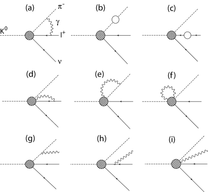
Figure 1: Feynman diagrams for the first-order radiative corrections to the $K^{0}_{\ell 3}$ decay mode. Diagrams (a)–(f) are the virtual corrections while diagrams (g)–(i) are the inner-bremsstrahlung corrections. The open circles in diagram (b) and (c) denote the self-energy correction to the pion and lepton wavefunctions, respectively.

Though higher-order corrections in $\alpha$, electromagnetic corrections to strong-interaction graphs, and weak interactions also contribute to the radiative correction, their effects are assumed to be small. For studies that model the effects of electromagnetic corrections to strong-interaction graphs, we refer the reader to the   studies [7, 8, 9].

To calculate the first-order radiative corrections, we need an expression for the “$K^{0}\pi^{-}\ell^{+}\nu_{\ell}$” effective vertex when at least one of the particle legs is off-shell [see Fig. 1(a), (g)–(h)]. Under ${\mathcal{A}}2$, the off-shell effective vertex is obtained from the on-shell phenomenological model. Therefore, the $K^{0}\pi^{-}\ell^{+}\nu_{\ell}$  vertex is

$$V^{K\pi\ell\nu}=i\sqrt{2}G_{F}V_{us}f_{+}(0)P_{R}\left[({p}\!\!\!/^{*}_{K}+{p}\!\!\!/^{*}_{\pi})\hat{f}_{+}(t^{*})+({p}\!\!\!/^{*}_{K}-{p}\!\!\!/^{*}_{\pi})\hat{f}_{-}(t^{*})\right],$$ (12)

where $p^{*}_{K}$ and $p^{*}_{\pi}$ are the (potentially) off-shell $K^{0}$ and $\pi^{-}$ four-momenta, $t^{*}=(p^{*}_{K}-p^{*}_{\pi})^{2}$, and the vector ${p}\!\!\!/$ denotes the contraction of the four-vector $p^{\mu}$ with the Dirac matrices, $\gamma^{\mu}$.

In general, one expects Eq. (12) to be an approximation of the true off-shell vertex. One potential correction to this vertex is a modification of the $K$–$\pi$ form factors. The form factors for the off-shell vertex may depend on kinematical quantities beyond $t$. In fact, using , Ref. [8] finds that the form factors depend on the additional variable $s=(p_{\pi}+p_{\ell})^{2}$ (e.g. $f_{\pm}(t,s)$). Since the emission of low-energy photons is expected to dominate the radiative corrections, we assume (${\mathcal{A}}3$) that the variation of the form factors $f_{+,\,0}$ is captured by simple $t$-dependence.

The expression for the off-shell $K^{0}\pi^{-}\ell^{+}\nu_{\ell}$  vertex may be simplified by using energy-momentum conservation and the Dirac equation for the neutrino. The simplified expression for this vertex is

$$V^{K\pi\ell\nu}=i\sqrt{2}G_{F}V_{us}f_{+}(0)P_{R}\left[2{p}\!\!\!/^{*}_{K}\hat{f}_{+}(t^{*})-{p}\!\!\!/^{*}_{\ell}\hat{f}_{2}(t^{*})\right],$$ (13)

where $\hat{f}_{2}(t^{*})=\hat{f}_{+}(t^{*})-\hat{f}_{-}(t^{*})$ is the difference between the $\hat{f}_{+}$ and $\hat{f}_{-}$ form factors.

We assume that the electromagnetic interaction with the pion is point-like (${\mathcal{A}}4$). Deviations from the point-like assumption are captured by the introduction of pion form factors. For experimental studies of the strength of pion form factors consult Ref. [14]; in this study, we assume pion form factors are negligible for current experimental sensitivities. Previous studies [22] of radiative corrections to the $K^{+}_{e3}\$decay mode include the effect of the pion form factors. Though the long-distance radiative correction to the $K^{+}_{e3}\$mode from Ref. [22] is larger in magnitude ($\delta_{LD}=-2\%$) than other studies that assume a point-like pion ($\delta_{LD}=-0.45\%$) [9, 18], the discrepancy is believed to be calculational rather than physical.

In Sec. 3.1.1 and Sec. 3.1.2 the matrix elements for the inner-bremsstrahlung contribution and the virtual contribution to the radiative corrections are calculated. The numerical methods used to evaluate the inner-bremsstrahlung and virtual matrix elements are discussed in Sec. 4.

3.1.1 Inner-Bremsstrahlung Contribution

Previous studies of single-photon radiation in $K^{0}_{\ell 3}\$decays using the aforementioned phenomenological model are found in Refs. [20, 21, 23, 24]. In Refs. [20, 21], the $K$–$\pi$ form factors were taken to be constant (${\mathcal{A}}5$) and the final state neutrino–photon system was assumed to be “undetected” (${\mathcal{A}}6$). Since the sensitivities of modern experiments are expected to probe the form factor dependence of $K^{0}_{\ell 3}\$decays, we relax ${\mathcal{A}}5$. Current experiments also measure the radiated photon from $K^{0}_{\ell 3}\$decays; therefore, we remove ${\mathcal{A}}6$ in our analysis.

In Refs. [23, 24], the $K^{0}_{\ell 3\gamma}$  matrix element was derived assuming a linear form factor model and using soft-photon theorems [32, 33]. Unlike Refs. [20, 21], their study does not assume that the photon is undetected; therefore, radiative photon spectra may be generated for use in detector-acceptance studies. In this section, we derive the inner-bremsstrahlung matrix element for the quadratic and the pole form factor models and we revisit the constant and linear models.

The inner-bremsstrahlung correction to the $K^{0}_{\ell 3}\$decay rate consists of single photon radiation from the pion, the lepton, and the effective vertex [see Fig. 1(g)–(i)]. The kinematics for the inner-bremsstrahlung diagrams are described by the decay equation,

$$K^{0}(p_{K})\rightarrow\pi^{-}(p_{\pi})\;\ell^{+}(p_{\ell})\;\nu_{\ell}(p_{\nu})\;\gamma(k),$$ (14)

where $k$ is the photon four-momentum.

Using the off-shell effective vertex, Eq. (13), the contribution to the inner-bremsstrahlung matrix element from radiation off the pion (Fig. 1(g)) and the lepton (Fig. 1(h)) is

$${\mathcal{M}}^{(g)+(h)} = e\sqrt{2}G_{F}V_{us}f_{+}(0)~{}\bar{u}(p_{\nu})P_{R}\left\{\left[2{p}\!\!\!/_{K}\hat{f}_{+}(t_{1})+m_{\ell}\hat{f}_{2}(t_{1})\right]\left[\frac{\epsilon^{*}(k)\cdot p_{\pi}}{k\cdot p_{\pi}}\right]\right.$$

$$-\left[2{p}\!\!\!/_{K}\hat{f}_{+}(t_{2})\right. + \left.m_{\ell}\hat{f}_{2}(t_{2})\right]\left.\left[\frac{\epsilon^{*}(k)\cdot p_{\ell}}{k\cdot p_{\ell}}+\frac{{k}\!\!\!/{\epsilon}\!\!\!/^{*}(k)}{2k\cdot p_{\ell}}\right]+\hat{f}_{2}(t_{2})\,{\epsilon}\!\!\!/^{*}(k)\right\}v(p_{\ell}),$$ (15)

where $\epsilon^{\mu}(k)$ is the photon polarization vector, $m_{\ell}$ is the mass of the charged lepton, and $\hat{f}_{2}(t)=\hat{f}_{+}(t)-\hat{f}_{-}(t)$. In Eq. (3.1.1), the form factors are evaluated for two different values of the momentum transfer to the $W^{+}$ gauge boson: $t_{1}$ and $t_{2}$. When the photon is radiated from the pion, the momentum transfer is $t_{1}=(p_{K}-p_{\pi}-k)^{2}=(p_{\ell}+p_{\nu})^{2}$ and when the photon is radiated from the charged lepton the momentum transfer is $t_{2}=(p_{K}-p_{\pi})^{2}$.

The last component of the inner-bremsstrahlung matrix element is from photon radiation off the effective vertex [see Fig. 1(i)]. The expression for the “$K^{0}\pi^{-}\ell^{+}\nu_{\ell}\gamma$” vertex is obtained by requiring the matrix element to be gauge invariant. In Ref. [20, 21] the $K^{0}\pi^{-}\ell^{+}\nu_{\ell}\gamma$  vertex is obtained by applying the principle of “minimal coupling” to the weak-interaction Lagrangian, while Refs. [23, 24] uses the Ward identity [34] to determine the $K^{0}\pi^{-}\ell^{+}\nu_{\ell}\gamma$  vertex. We illustrate both of these methods and we use the latter to determine the forms of the $K^{0}\pi^{-}\ell^{+}\nu_{\ell}\gamma$  vertex for non-constant form factors.

Assuming the form factors are constant, the weak-interaction Lagrangian is

$${\mathcal{L}}_{W}=\sqrt{2}G_{F}V_{us}~{}\bar{\psi_{\nu}}\gamma^{\mu}P_{L}\psi_{\ell}~{}\left[(f_{+}+f_{-})\phi_{\pi}\partial_{\mu}\phi_{K}+(f_{+}-f_{-})\phi_{K}\partial_{\mu}\phi_{\pi}\right],$$ (16)

where $\psi$ and $\phi$ denote the fermion and complex scalar fields, respectively. Replacing the partial derivative with the covariant derivative (minimal coupling),

$$\partial_{\mu}\rightarrow D_{\mu}=\partial_{\mu}-ieQA_{\mu},$$ (17)

where $A_{\mu}$ is the photon field, one obtains the $K^{0}\pi^{-}\ell^{+}\nu_{\ell}\gamma$  effective vertex,

$$V^{K\pi\ell\nu\gamma,\;\mu}_{\rm cons} = -i\sqrt{8\pi\alpha}\;G_{F}V_{us}P_{R}\;f_{2}\gamma^{\mu}.$$ (18)

Combining all three inner-bremsstrahlung graphs, the matrix element for the constant form factors is

$${\mathcal{M}}_{\rm cons}^{\rm brem}=e\sqrt{2}G_{F}V_{us}f_{+}(0)\;\bar{u}(p_{\nu})P_{R}\left[2{p}\!\!\!/_{K}+m_{\ell}\right]\left[\frac{\epsilon^{*}(k)\cdot p_{\pi}}{k\cdot p_{\pi}}-\frac{\epsilon^{*}(k)\cdot p_{\ell}}{k\cdot p_{\ell}}-\frac{{k}\!\!\!/{\epsilon}\!\!\!/^{*}(k)}{2k\cdot p_{\ell}}\right]v(p_{\ell}).$$ (19)

Since $\hat{f}_{+,\,2}$ are normalized and independent of $t$ they have been set to $1$. Taking $\epsilon^{\mu}(k)\rightarrow k^{\mu}$ in Eq. (19), one observes that ${\mathcal{M}}_{\rm cons}^{\rm brem}\rightarrow 0$ and therefore the Ward identity is satisfied.

Extraction of the $K^{0}\pi^{-}\ell^{+}\nu_{\ell}\gamma$  vertex through minimal coupling works well for the constant form factor model. When form factors are no longer constant and when the matrix element depends on two different values of $t$ (e.g. $t_{1}$ and $t_{2}$), this method is insufficient. For this scenario, we determine the $K^{0}\pi^{-}\ell^{+}\nu_{\ell}\gamma$  vertex by requiring the inner-bremsstrahlung matrix element to be zero when the photon polarization vector $\epsilon^{\mu}(k)$ is replaced by the photon four-momentum (Ward identity). This method does not uniquely determine the $K^{0}\pi^{-}\ell^{+}\nu_{\ell}\gamma$  vertex; the vertex expression may differ by structure-dependent terms. For a discussion of structure-dependent terms we refer the reader to Ref. [23, 24].

Using this methodology, the $K^{0}\pi^{-}\ell^{+}\nu_{\ell}\gamma$  vertex for the linear form factor model is

$$V^{K\pi\ell\nu\gamma,~{}\mu}_{\rm lin}=-i\sqrt{8\pi\alpha}\;G_{F}V_{us}f_{+}(0)P_{R}\left\{\hat{f}_{2}(t_{2})\,\gamma^{\mu}-2\hat{f}^{\prime}_{+}(0)\left[2{p}\!\!\!/_{K}-{p}\!\!\!/_{\ell}\right](p_{K}-p_{\pi})^{\mu}\right\},$$ (20)

where $\hat{f}^{\prime}_{+}(0)$ ($=\lambda_{+}/m_{\pi}^{2}$) is the slope of the normalized form factor. The vertex interaction for the quadratic model is

$$\begin{array}[]{ll}\lx@intercol V^{K\pi\ell\nu\gamma,\,\mu}_{\rm quad}=-i\sqrt{8\pi\alpha}\;G_{F}V_{us}f_{+}(0)P_{R}\left\{\hat{f}_{2}(t_{2})\;\gamma^{\mu}\right.\hfil\lx@intercol\\ &-2\left[2{p}\!\!\!/_{K}-{p}\!\!\!/_{\ell}\right]\left[\hat{f}^{\prime}_{+}(0)+\frac{1}{2}(t_{1}+t_{2})\hat{f}^{\prime\prime}_{+}(0)\right](p_{K}-p_{\pi})^{\mu}\\ &-\left.{p}\!\!\!/_{\ell}(m_{K}^{2}-m_{\pi}^{2})\left[\hat{f}^{\prime\prime}_{0}(0)-\hat{f}^{\prime\prime}_{+}(0)\right](p_{K}-p_{\pi})^{\mu}\right\},\end{array}$$

where $\hat{f}^{\prime}_{+,\,0}(0)$ ($=\lambda^{\prime}_{+,\,0}/m_{\pi}^{2}$) and $\hat{f}^{\prime\prime}_{+,\,0}(0)$ ($=\lambda^{\prime\prime}_{+,\,0}/m_{\pi}^{4}$). The vertex interaction for the pole model is

$$\begin{array}[]{ll}\lx@intercol V^{K\pi\ell\nu\gamma,~{}\mu}_{\rm pole}=-i\sqrt{8\pi\alpha}~{}G_{F}V_{us}f_{+}(0)P_{R}\left\{\hat{f}_{2}(t_{2})\;\gamma^{\mu}\right.\hfil\lx@intercol\\ &-2\left[2{p}\!\!\!/_{K}-{p}\!\!\!/_{\ell}\right]D_{+}(t_{1},t_{2})(p_{K}-p_{\pi})^{\mu}\\ &-2{p}\!\!\!/_{\ell}(m_{K}^{2}-m_{\pi}^{2})\left(\frac{m^{2}_{+}-m^{2}_{0}}{m^{2}_{+}m^{2}_{0}}\right)(p_{K}-p_{\pi})^{\mu}\\ &\;\;\;\;\left.\times\left[f_{0}(t_{1})D_{+}(t_{1},t_{2})+f_{+}(t_{2})D_{0}(t_{1},t_{2})\right]\right\},\end{array}$$ (21)

where $m_{+}$ and $m_{0}$ are the poles of the $K^{*}$ mesons and

$$D_{+,\,0}(t_{1},t_{2}) = m^{-2}_{+,\,0}\,f_{+,\,0}(t_{1})f_{+,\,0}(t_{2}).$$ (22)

Combining the $K^{0}\pi^{-}\ell^{+}\nu_{\ell}\gamma$  contribution with Eq. (3.1.1), the inner-bremstrahlung matrix element is

$${\mathcal{M}}^{\rm brem} = e\sqrt{2}G_{F}V_{us}f_{+}(0)\,\bar{u}(p_{\nu})P_{R}\left\{\left[2{p}\!\!\!/_{K}\hat{f}_{+}(t_{1})+m_{\ell}\hat{f}_{2}(t_{1})\right]\left[\frac{\epsilon^{*}(k)\cdot p_{\pi}}{k\cdot p_{\pi}}\right]\right.$$ (23)

$$- \left.\left[2{p}\!\!\!/_{K}\hat{f}_{+}(t_{2})+m_{\ell}\hat{f}_{2}(t_{2})\right]\left[\frac{\epsilon^{*}(k)\cdot p_{\ell}}{k\cdot p_{\ell}}+\frac{{k}\!\!\!/{\epsilon}\!\!\!/^{*}(k)}{2k\cdot p_{\ell}}\right]+{\mathcal{X}}\right\}v(p_{\ell}),$$

where ${\mathcal{X}}$ is non-zero for non-constant form factor models. The three following equations define ${\mathcal{X}}$ for the linear, the quadratic, and the pole model:

$$\begin{array}[]{lcl}{\mathcal{X}}_{\rm lin}&=&2\xi\hat{f}^{\prime}_{+}(0)\left[2{p}\!\!\!/_{K}-{p}\!\!\!/_{\ell}\right]\\ {\mathcal{X}}_{\rm quad}&=&2\xi\left[2{p}\!\!\!/_{K}-{p}\!\!\!/_{\ell}\right]\left[\hat{f}^{\prime}_{+}(0)+\frac{1}{2}(t_{1}+t_{2})\hat{f}^{\prime\prime}_{+}(0)\right]-\xi{p}\!\!\!/_{\ell}(m_{K}^{2}-m_{\pi}^{2})\left[\hat{f}^{\prime\prime}_{+}(0)-\hat{f}^{\prime\prime}_{0}(0)\right]\\ {\mathcal{X}}_{\rm pole}&=&2\xi\left[2{p}\!\!\!/_{K}-{p}\!\!\!/_{\ell}\right]D_{+}(t_{1},t_{2})\\ &&+2\xi{p}\!\!\!/_{\ell}(m_{K}^{2}-m_{\pi}^{2})\left(\frac{m^{2}_{+}-m^{2}_{0}}{m^{2}_{+}m^{2}_{0}}\right)\left[f_{0}(t_{1})D_{+}(t_{1},t_{2})+f_{+}(t_{2})D_{0}(t_{1},t_{2})\right],\end{array}$$ (24)

where $\xi=\epsilon^{*}(k)\cdot(p_{K}-p_{\pi})$, and $m_{+}$ and $m_{0}$ are the vector and scalar $K^{*}$ masses of the pole form factor model.

The terms in Eq. (24) are necessary to maintain the gauge invariance of the matrix element. In our numerical evaluation of the inner-bremsstrahlung matrix element [see Sec. 4], we introduce a small photon mass $\lambda$ to regulate the infrared divergence. If the contribution from Fig. 1(i) to the matrix element was not included, then the matrix element would grow like $\sim E_{\gamma}/\lambda$. This behavior arises from the longitudinal component of the photon polarization vector in the term $f_{2}(t_{2}){\epsilon}\!\!\!/(k)$ and also from the the fact that $t_{1}\neq t_{2}$. Including the effect of Fig. 1(i) in the matrix element, the Ward identity is maintained and the matrix element has the correct behavior as the photon mass, $\lambda$, goes to zero.

3.1.2 Virtual Contribution

The first-order virtual corrections consist of three types of diagrams: self-energy corrections (Fig. 1(b)–(c)), inter-particle photon exchange (Fig. 1(a)), and effective vertex interactions (Fig. 1(d)–(f)). Previous studies [20, 21] calculate the virtual corrections assuming that the form factors are constant. In this section, we recalculate the virtual matrix element assuming constant form factors and we investigate two methods to calculate the virtual contribution for non-constant form factors.

Self-energy corrections to the pion and to the charged lepton are obtained by wavefunction renormalization of the weak Lagrangian [see Eq. (16)]. The wavefunction renormalizations for the pion and the charged lepton are

$$\delta Z_{\ell} = \frac{\alpha}{4\pi}\left[2B_{1}(m^{2}_{\ell};m^{2}_{\ell},\lambda^{2})+4m^{2}_{\ell}B^{\prime}_{1}(m^{2}_{\ell};m^{2}_{\ell},\lambda^{2})+8m^{2}_{\ell}B^{\prime}_{0}(m^{2}_{\ell};m^{2}_{\ell},\lambda^{2})\right]$$ (25)

$$\delta Z_{\pi} = \frac{\alpha}{4\pi}\left[1+2B_{0}(m^{2}_{\pi};m^{2}_{\pi},\lambda^{2})+(4m^{2}_{\pi}-\lambda^{2})B^{\prime}_{0}(m^{2}_{\pi};m^{2}_{\pi},\lambda^{2})\right],$$ (26)

where $B(\cdot)$ and $B^{\prime}(\cdot)$ are the two-point loop integral [42] and its derivative,
$B^{\prime}(p_{1}^{2},m_{0}^{2},m_{1}^{2})=\partial B(p_{1}^{2},m_{0}^{2},m_{1}^{2})/\partial p_{1}^{2}$. The loop integrals are calculated using a cutoff regularization and are defined in Appendix A. The self-energy contribution to the virtual matrix element is

$${\mathcal{M}}^{(b)+(c)} = \frac{1}{2}(\delta Z_{\ell}+\delta Z_{\pi}){\mathcal{M}}^{B},$$ (27)

where ${\mathcal{M}}^{B}$ is the lowest-order $K^{0}_{\ell 3}\$matrix element [see Eq. (2)].

The inter-particle photon exchange diagram is calculated using Eq. (13) for the $K^{0}\pi^{-}\ell^{+}\nu_{\ell}$  vertex. Since the form factors are assumed constant, they may be pulled outside of the photon four-momentum integration. For non-constant form factor models, the form factors will depend on the photon four-momentum and directly modify the photonic loop integration.

For the constant form factor model, the vertex correction consists of the diagrams (d) and (e) of Fig. 1. Since the minimal coupling anzatz does not require a $K^{0}\pi^{-}\ell^{+}\nu_{\ell}\gamma\gamma$  vertex, Fig. 1(f) is neglected in the virtual correction calculation. The $K^{0}\pi^{-}\ell^{+}\nu_{\ell}\gamma$  vertex from Eq. (19) is used to calculate the effective vertex interaction graphs. As with the evaluation of the inter-particle photon exchange diagram, the constant form factor does not modify the integral over the photon four-momenta.

Combining the contributions from each of the virtual diagrams, the virtual matrix element for a constant form factor model is

$${\mathcal{M}}^{\rm virt}=\frac{\alpha}{4\pi}\sqrt{2}G_{F}V_{us}f_{+}(0)~{}\bar{u}(p_{\nu})P_{R}\left[A{p}\!\!\!/_{K}-B{p}\!\!\!/_{\ell}\ \right]v(p_{\ell}),$$ (28)

where $A$ and $B$ may be written in terms of photon loop integrals. $A$ and $B$ are given by the equations

$$\begin{array}[]{ll}\lx@intercol A=\;\;\hat{f}_{+}\left[1+4B_{0}(m^{2}_{\pi};m^{2}_{\pi},\lambda^{2})+2B_{1}(m^{2}_{\ell};m^{2}_{\ell},\lambda^{2})\right.\hfil\lx@intercol\\ &\left.+(4m^{2}_{\pi}-\lambda^{2})B^{\prime}_{0}(m^{2}_{\pi};m^{2}_{\pi},\lambda^{2})\right.\\ &\left.+8m^{2}_{\ell}B^{\prime}_{0}(m^{2}_{\ell};m^{2}_{\ell},\lambda^{2})+4m^{2}_{\ell}B_{1}^{\prime}(m^{2}_{\ell};m^{2}_{\ell},\lambda^{2})\right.\\ &\left.-8x_{\pi\ell}\,C_{0}+4m^{2}_{\pi}C_{1}-4\left(2x_{\pi\ell}+m^{2}_{\ell}\right)C_{2}\right]\\ \lx@intercol\hskip 19.91692pt+\hat{f}_{2}\left[2B_{0}(s_{\pi\ell};m^{2}_{\pi},m^{2}_{\ell})-B_{0}(m^{2}_{\pi};m^{2}_{\pi},\lambda^{2})\right.\hfil\lx@intercol\\ &\left.+4B_{0}(m^{2}_{\ell};m^{2}_{\ell},\lambda^{2})+2B_{1}(m^{2}_{\ell};m^{2}_{\ell};\lambda^{2})\right.\\ &\left.+B_{1}(m^{2}_{\pi};m^{2}_{\pi},\lambda^{2})+B_{1}(m^{2}_{\pi};\lambda^{2},m^{2}_{\pi})\right.\\ &\left.+2\lambda^{2}C_{0}-4x_{\pi\ell}\,C_{1}+2m^{2}_{\ell}C_{2}\right]\\ \end{array}$$ (29)

and

$$\begin{array}[]{ll}\lx@intercol B=\;\;\hat{f}_{+}\left[-4s_{\pi\ell}\,C_{2}\right]\hfil\lx@intercol\\ \lx@intercol\hskip 19.91692pt+\hat{f}_{2}\left[\frac{1}{2}+2B_{0}(s_{\pi\ell};m^{2}_{\pi},m^{2}_{\ell})+B_{0}(m^{2}_{\pi};\lambda^{2},m^{2}_{\pi})\right.\hfil\lx@intercol\\ &\left.-4B_{0}(m^{2}_{\ell};m^{2}_{\ell},\lambda^{2})+B_{1}(m^{2}_{\pi};m^{2}_{\pi},\lambda^{2})\right.\\ &\left.+B_{1}(m^{2}_{\pi};\lambda^{2},m^{2}_{\pi})-B_{1}(m^{2}_{\ell};m^{2}_{\ell},\lambda^{2})\right.\\ &\left.+4m^{2}_{\ell}B^{\prime}_{0}(m^{2}_{\ell};m^{2}_{\ell},\lambda^{2})\right.\\ &\left.+\frac{1}{2}(4m^{2}_{\pi}-\lambda^{2})B^{\prime}_{0}(m^{2}_{\pi};m^{2}_{\pi},\lambda^{2})\right.\\ &\left.+2m^{2}_{\ell}B^{\prime}_{1}(m^{2}_{\ell};m^{2}_{\ell},\lambda^{2})\right.\\ &\left.+(2\lambda^{2}-4x_{\pi\ell})C_{0}+(2m^{2}_{\pi}-4x_{\pi\ell})C_{1}\right.\\ &\left.+(2m^{2}_{\ell}-4x_{\pi\ell})C_{2}\right]\\ \end{array}$$ (30)

where $s_{ij}=(p_{i}+p_{j})^{2}$, $x_{ij}=p_{i}\cdot p_{j}$, and $C_{i}=C_{i}(m^{2}_{\pi},s_{\pi\ell},m^{2}_{\ell};\lambda^{2},m^{2}_{\pi},m^{2}_{\ell})$.

In Eq. (29)–(30), a small photon mass $\lambda$ is introduced to regulate the infrared (IR) divergence. Since the $K^{0}\pi^{-}\ell^{+}\nu_{\ell}$  vertex is an effective interaction, the interaction is not renormalizable and will depend on an ultraviolet (UV) cutoff scale, $\Lambda$. Assuming a constant form factor model, the virtual matrix element is logarithmically divergent (${\mathcal{M}}^{\rm virt}\sim\ln\Lambda^{2}$). A cutoff regulator is used when calculating the loop integrals; we select the UV cutoff such that $\Lambda>m_{\pi},\,m_{\ell}$. We take $\Lambda$ to be the proton mass ($m_{p}$). In Sec. 5, we discuss the sensitivity of the radiative correction to the UV cutoff scale.

For non-constant form factors, Eq. (29)–(30) will be modified. In this paper, we use two methods to study the effects of non-constant form factors in the virtual calculation. The first method, Method I, is an approximate method in which the constant form factors $f_{+,\,0}$ in Eq. (29)–(30) are replaced by $f_{+,\,0}(t)$, where $t=(p_{K}-p_{\pi})^{2}$. Using this method, each $K^{0}_{\ell 3}\$event is modified based on the size of the momentum transfer to the lepton–neutrino system.

The second method, Method II, assumes the pole form factor model and it includes the effect of the photon four-momenta on the form factor. For instance, in the inter-particle photon exchange diagram (Fig. 1(a)), the form factor depends on the momentum transfer $t_{1}=(p_{K}-p_{\pi}-k)^{2}$. Therefore, the $k$-dependence of the form factor will modify the photonic loop integration. Expressions for $A$ and $B$ in the Method II are in Appendix B. For Method II, we also use cutoff regularization; therefore, a new UV cutoff scale is selected that is larger than the mass of the $K^{*}$ poles.

Results from both methods are presented in Sec. 5.

4 Numerical Methods

To determine a numerical value for the long-distance radiative correction, $\delta^{\ell}_{LD}$, we integrate the squared, summed inner-bremsstrahlung and virtual matrix elements over their respective final-state phase spaces. To aid in this evaluation, we developed a program named KLOR (Kaon Leading Order Radiation). Using KLOR, we numerically evaluate the inner-bremsstrahlung and the virtual matrix elements for both constant and non-constant form factor models. In this section, we discuss the methodology of the numerical calculation.

Using the expressions for the inner-bremsstrahlung and the virtual matrix elements in Sec. 3, KLOR numerically squares each matrix element and sums each of them over polarization- and spin- states. The squared, summed matrix elements are integrated over phase space by two methods: Vegas integration [35] and traditional Monte Carlo integration [36]. The Vegas integration is used to evaluate the total decay rate, while the traditional Monte Carlo integration is used to check the Vegas integration and to evaluate the decay rate when final-state requirements on the photon kinematics (e.g. angular and/or energy constraints) are imposed. An optimized, phase-space sampling technique is used to efficiently generate unweighted event samples.

Since our calculation of the decay rate is numerical, proper regulation of the IR divergence is necessary to obtain finite results. The IR divergence is regulated by introducing a small photon mass $\lambda$. For the inner-bremsstrahlung calculation, the photon mass limits the kinematically accessible four-body phase space. Since the photon is massive, one needs to sum over the longitudinal polarization in addition to the two transverse polarizations. In the virtual calculation, the photon mass modifies the loop integration over the photon momentum. Tests of the numerical stability of our IR regularization scheme show that KLOR’s results are numerically stable for photon masses from $\sim 10^{-5}$ to $10^{-14}$ GeV/c².

The phenomenological $K^{0}\pi^{-}\ell^{+}\nu_{\ell}$  interaction is effective (non-renormalizable); therefore, this model describes the interaction up to a UV cutoff scale, $\Lambda$. We take the UV cutoff, $\Lambda$, to be the low-energy cutoff described in Sec. 3; recall that the low-energy cutoff is the boundary between the long- and short- distance corrections. The UV cutoff is used to regulate the loop integration – cutoff regularization. In particular, the photon energy is integrated up to the UV scale $\Lambda$.

Loop integrals in the virtual matrix element are computed using the numerical package Looptools [37, 38]. Looptools calculates the value of loop integrals using analytic expressions derived for dimensional regularization. As long as the cutoff scale is taken to be large; evaluation of the loop integrals in the cutoff regularization can be related to the corresponding expressions in dimensional regularization with minor modifications.

In Appendix C, we compare results from KLOR to other approximate techniques. In particular, we analyze distributions produced by KLOR and another program called PHOTOS [10]. PHOTOS is a Monte Carlo event generator that can be used to approximate the radiative corrections to the $K^{0}_{\ell 3}\$decay modes.

5 Results

In Sec. 3, we developed a phenomenological framework to describe radiative corrections to the $K^{0}_{\ell 3}\$decay modes and in Sec. 4, we described a program, KLOR, that was written to implement this framework. In this section, we use KLOR to illustrate the structure of the corrections, to determine the $\delta^{\ell}_{LD}$  parameter, and to calculate experimentally measurable observables of the model.

Before delving into the aforementioned topics, we would like to illustrate the size of the radiative corrections. One approach is to examine the invariant mass of the pion/lepton system, denoted $m_{\pi\ell}$. In Fig. 2, we plot the Born and the next-to-leading order (NLO) differential decay rates as a function of $m_{\pi e}$ (Fig. 2(a)) and $m_{\pi\mu}$ (Fig. 2(b)). In the notation of Eq. (10), the Born decay rate is $\Gamma^{(0)}_{K\ell 3}$ and the NLO decay rate is $\Gamma^{(0)}_{K\ell 3}+\Gamma^{(1)}_{K\ell 3}$.

The effect of radiative corrections on the Born decay rate is illustrated by the shifts of the NLO distribution from the Born distribution. In Fig. 2(c) and Fig. 2(d), we plot the ratio of the NLO and the Born $m_{\pi\ell}$ distributions for the $K^{0}_{e3}\$and $K^{0}_{\mu 3}\$modes, respectively. In each of these plots, we assume a pole model [see Eq. (6)] for the hadronic $K$–$\pi$ form factors. The parameters of the pole model, $m_{+}=0.882$ GeV/c² and $m_{0}=1.174$ GeV/c² are from a recent measurement by the KTeV Collaboration [6].

As observed in Fig. 2, radiative corrections do not uniformly modify the $m_{\pi e}$ distribution. Radiative corrections enhance the Born decay rate for $m_{\pi e}$ masses below $0.3$ GeV/c² and suppress the Born decay rate for $m_{\pi e}$ masses above $0.3$ GeV/c². A typical correction to the $m_{\pi e}$ distribution is $\sim 5\%$ but can be greater for $m_{\pi e}$ masses near the kinematic boundaries. Radiative corrections to the $m_{\pi\mu}$ distribution tend to be more uniform and generally enhance the decay rate. A typical $K^{0}_{\mu 3}\$correction to the $m_{\pi\mu}$ distribution is $\sim 3\%$ but can be larger near the endpoints of the $m_{\pi\mu}$ distribution.

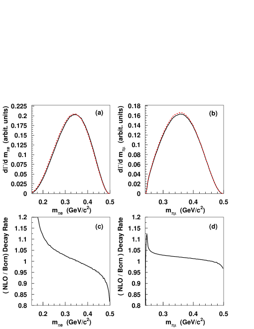
Figure 2: (a) The invariant mass distribution of the pion–electron system ($m_{e\pi}$) using the Born (solid line) and the NLO (dashed line) matrix elements. (b) The invariant mass distribution of the pion–muon system ($m_{\mu\pi}$) using the Born (solid line) and the NLO (dashed line) matrix elements. (c) and (d) are the ratio of the NLO and the Born distributions for the $m_{e\pi}$ and $m_{e\pi}$ distributions, respectively.

Now that we have a basic understanding of the size of the radiative corrections in the $K^{0}_{e3}\$and the $K^{0}_{\mu 3}\$modes, we investigate the structure of the radiative corrections. In particular, we study radiative corrections over the $K^{0}_{e3}\$and the $K^{0}_{\mu 3}\$three-body Dalitz regions.

5.1 Dalitz Distribution of the Radiative Corrections

In Fig. 3(a) and Fig. 4(a), we plot the lowest-order decay rates for the $K^{0}_{e3}\$and the $K^{0}_{\mu 3}\$decay modes over their respective three-body Dalitz regions. These plots illustrate the dependence of the Born decay rate on the reduced energies

$$y=\frac{2E_{\pi}}{m_{K}} z=\frac{2E_{\ell}}{m_{K}},$$ , (31)

where $E_{\pi}$ ($E_{\ell}$) is the pion (charged lepton) energy in the kaon center of mass.

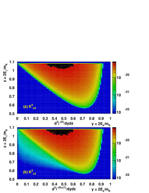
Figure 3: (a) Dalitz plot of the Born decay rate for the $K^{0}_{e3}\$mode. (b) Dalitz plot for the $K^{0}_{e3}\$decay rate including radiative corrections. Plot (b) uses the pole form factor model ($m_{+}=0.882$ GeV/c², $m_{0}=1.174$ GeV/c²) [6] and Method I to calculate the virtual diagrams. The cutoff scale $\Lambda=m_{p}$ is used.

When radiative effects are included, the Born Dalitz distributions are modified. Using Method I [see Sec. 3.1.2], the NLO decay rate for the $K^{0}_{e3}\$and $K^{0}_{\mu 3}\$modes are plotted in Fig. 3(b) and Fig. 4(b), respectively. In general, radiative corrections modify the Born decay rate both inside and outside the Dalitz region. Inside the Dalitz region, both virtual and inner-bremsstrahlung diagrams contribute to the NLO decay rate; while outside the Dalitz region, only inner-bremsstrahlung diagrams contribute. The inner-bremsstrahlung contribution to the $K^{0}_{\ell 3}\$decay rate outside the Dalitz region is more pronounced in the $K^{0}_{e3}\$decay mode than in the $K^{0}_{\mu 3}\$decay mode since there is a higher probability of radiation from the electron.

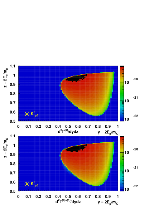
Figure 4: (a) Dalitz plot of the Born decay rate for the $K^{0}_{\mu 3}\$mode. (b) Dalitz plot for the $K^{0}_{\mu 3}\$decay rate including the radiative corrections. Plot (b) uses the pole form factor model ($m_{+}=0.882$ GeV/c², $m_{0}=1.174$ GeV/c²) [6] and Method I to calculate the virtual diagrams. The cutoff scale $\Lambda=m_{p}$ is used.

The long-distance radiative correction to each point in the three-body Dalitz plane, denoted $\delta^{\ell}_{LD}(y,z)$, may be obtained by taking the ratio of the NLO and the Born distributions and then subtracting unity. $\delta^{\ell}_{LD}(y,z)$ is interesting since it describes the structure of the radiative correction; for a given ($E_{\pi}$, $E_{\ell}$), $\delta^{\ell}_{LD}(y,z)$ characterizes how the Born distribution is modified.

In Fig. 5, we plot $\delta^{\ell}_{LD}(y,z)$ using Method I for both the $K^{0}_{e3}\$and the $K^{0}_{\mu 3}\$modes. Radiative corrections to the $K^{0}_{e3}\$Dalitz region can be significant, ranging from $-15$% to $15$%. Radiative corrections to the $K^{0}_{\mu 3}\$Dalitz region are smaller than for the $K^{0}_{e3}\$mode; they range from $-2$% to $8$%. Since there is no contribution to the Born decay rate from outside the Dalitz region, $\delta^{\ell}_{LD}(y,z)$ is infinite in this region. In Fig. 5, we have set $\delta^{\ell}_{LD}(y,z)$ outside the Dalitz region to zero. Depending on the technique used to measure the $K^{0}_{\ell 3}\$decay rate, the contribution from outside the Dalitz region may need to be included in the $\delta^{\ell}_{LD}$  calculation. In Sec. 5.2, we address this and other issues affecting the $\delta^{\ell}_{LD}$  calculation.

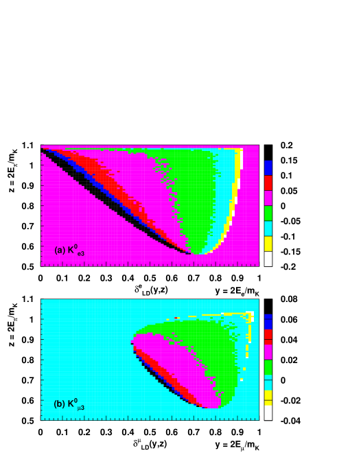
Figure 5: Long-distance radiative correction, $\delta^{\ell}_{LD}$, to $K^{0}_{e3}\$(a) and the $K^{0}_{\mu 3}\$(b) Dalitz plots. Both plots use the pole form factor model ($m_{+}=0.882$ MeV/c², $m_{0}=1.174$ MeV/c²) [6] and Method I to calculate the virtual diagrams. The UV cutoff ($\Lambda$) for the long-distance calculation is taken to be the proton mass.

Before we calculate $\delta^{\ell}_{LD}$, we compare the two methods, Method I and Method II, proposed in Sec. 3.1.2. Recall that Method I and Method II are two ways to introduce non-constant form factors into the virtual matrix element calculation. We compare these methods by generating radiative distributions and examining the differences between them.

In Fig. 6(a), we plot the difference between the NLO and Born decay rate as a function of $m_{\pi e}$. The solid (dashed) line is produced using Method I (Method II). The $m_{\pi e}$ distribution using Method II is shifted higher than that produced by Method I; however, the size and structure of the distributions are similar.

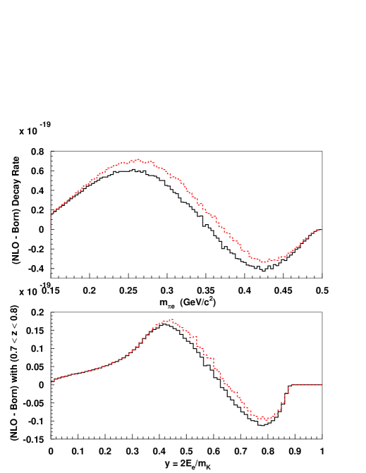
Figure 6: (a) The $m_{\pi e}$ distribution of the difference between the NLO and the Born $K^{0}_{e3}\$decay rates. Method I (solid) and Method II (dashed) are presented. (b) The $y$ distribution of the difference between the NLO and the Born $K^{0}_{e3}\$decay rates in the $0.7<z<0.8$ band of the $K^{0}_{e3}\$Dalitz plane. Method I (solid) and Method II (dashed) are presented.

In Fig. 6(b), we plot the $y$ ($=2E_{e}/m_{K}$) distribution for the difference between the NLO and Born decay rates in the $0.7<z<0.8$ “band” of the Dalitz plane. As with the $m_{\pi e}$ distribution, the radiative correction from the Method I and Method II have very similar sizes and shapes. Inspection of other bands in the Dalitz plane lead to similar findings.

Since the radiative correction distributions produced by Method I and Method II produce commensurate spectra, one expects that the distribution of $K^{0}_{\ell 3}\$events produced by Method I and Method II to be identical for current experimental precision. The distributions from Method II are in general more positive than those of Method I; therefore, we expect that the total radiative correction for Method II to be slightly larger.

5.2 The $\delta^{\ell}_{LD}$  Parameter

The total radiative correction, denoted $\delta^{\ell}_{T}$, to the Born $K^{0}_{\ell 3}\$decay rate consists of a short- and long-distance component. Using the phenomenological model [see Sec. 3], we calculate $\delta^{\ell}_{LD}$  and estimate its uncertainty. Before we can determine $\delta^{\ell}_{LD}$, we must first specify the analysis technique used by experimentalists to measure the $K^{0}_{\ell 3}\$decay rate.

In previous studies [20, 21, 8], the authors assume that the experimental apparatus only measures the charged lepton and the pion; the neutrino and (if present) the photon are “invisible.” The observed pion and charged lepton momenta are then fit to three-body kinematics with zero missing mass. If a $K^{0}_{\ell 3}\$event produces a ‘$\ell\pi$’ signature that lies outside the three-body Dalitz region, then it is excluded from the decay rate measurement. Note that this scenario only works for an ideal experiment for which the kaon energy is known and where the analysis cuts are such that events can not migrate from outside the three-body Dalitz region. For this experimental analysis technique, the long-distance radiative correction parameter is the total correction to the Born decay rate inside the three-body $K^{0}_{\ell 3}\$Dalitz region. In this scenario, we denote the long-distance radiative correction $\hat{\delta}^{\ell}_{LD}$.

We consider an experimentally motivated approach to the analysis in which the experiment is sensitive to and detects radiated photons in the final state. Therefore, an analysis of the $K^{0}_{\ell 3}\$decay rate will include radiated photons. Moreover, we also assume the experimental analysis includes $K^{0}_{\ell 3}\$signatures with measured pion and charged lepton energies outside the three-body Dalitz region. In this analysis, $\delta^{\ell}_{LD}$  includes contributions from both inside and outside the three-body Dalitz plot [see Fig. 3]. Note that since we perform a numerical analysis [see Sec. 4], one can compute $\hat{\delta}^{\ell}_{LD}$, which excludes events from outside the three-body Dalitz region.

In addition to the experimental technique, $\delta^{\ell}_{LD}$  will depend on the cutoff scale $\Lambda$. As described in Sec. 3, both the short- and long-distance radiative corrections depend on the scale $\Lambda$ which denotes the “boundary” between the short- and long-distance loop corrections. Below $\Lambda$, radiative corrections to the $K^{0}_{\ell 3}\$decay rate are described by the phenomenological model; while, above $\Lambda$, radiative corrections are described by the Standard Model. In our analysis, we associate uncertainty in the total radiative correction ($\delta^{\ell}_{T}$) due to the cutoff scale choice with uncertainty in the long-distance radiative correction.

The choice of the cutoff scale is somewhat arbitrary and typically depends on the “physics” and the calculational limitations of the long-distance model. Since we use the cutoff regulator to compute the loop integrals, we take $\Lambda$ to be larger than the masses appearing in the loop integrals. In Method I and Method II, we take $\Lambda$ to be $m_{p}$ and $3$ GeV/c², respectively. Though the assumption that the long-distance model describes physics at the cutoff scale $\Lambda=3$ GeV/c² is likely optimistic, integration of the loop integrals, which depend on the $K^{*}$ poles, requires a higher cutoff scale.

In Table 1 and Table 2, we compute the short- and long-distance radiative corrections for various cutoff scales ranging from $m_{\rho}$ ($=0.7711$ GeV/c²) to $3$ GeV/c². For Method I, changing the cutoff scale from $m_{\rho}$ to $3$ GeV/c² results in changes to $\delta^{e}_{LD}$  , $\delta^{\mu}_{LD}$  , and to $\delta_{SD}$  of $\sim 0.7\%$; however, $\delta^{e}_{T}$  ($=\delta_{SD}+\delta^{e}_{LD}$) remains stable to within $\sim 0.2\%$. Therefore, a reasonable uncertainty in $\delta^{e}_{LD}$  due to the cutoff scale uncertainty is $0.2\%$. A similar inspection of the $K^{0}_{\mu 3}\$mode indicates an uncertainty to $\delta^{\mu}_{LD}$  from the cutoff scale is $0.1\%$.

In addition to the uncertainty associated with the cutoff scale ambiguity, there is an uncertainty in the radiative corrections due to the method used to calculate the virtual corrections. Using Method II, the total radiative corrections to the $K^{0}_{e3}\$and the $K^{0}_{\mu 3}\$modes are slightly larger than the corresponding values obtained via Method I. Therefore, for $\delta^{e}_{LD}$  and $\delta^{\mu}_{LD}$  we take an additional uncertainty of $0.1\%$ and $0.2\%$ due to the method that is used to calculate the virtual corrections.

Therefore, after inspection of the shifts to the total radiative corrections in Table 1 and Table 2, we take the uncertainty on the long-distance radiative corrections due to the cutoff scale and the virtual calculation method to be $0.3\%$ for both $\delta^{e}_{LD}$  and $\delta^{\mu}_{LD}$.

Table 1: Long- and short-distance [39] radiative corrections to the $K^{0}_{e3}\$decay modes. Results are presented for different virtual correction methods (I and II), for different form factor models, and for various UV cutoff scales. We use the measured values of the form factor parameters taken from Ref. [6].

FF Model	$\Lambda$	$\delta_{SD}$	$\delta^{e}_{LD}$	$\delta^{e}_{T}$
	(GeV/c2)	(%)	(%)	(%)
Method I
Constant	$m_{\rho}$	2.27	1.26	3.53
Constant	$m_{p}$	2.17	1.31	3.48
Constant	$2m_{p}$	1.94	1.55	3.49
Constant	$3$	1.64	1.73	3.37
Linear	$m_{p}$	2.17	1.32	3.49
Quadratic	$m_{p}$	2.17	1.33	3.50
Pole	$m_{p}$	2.17	1.33	3.50
Method II
Pole	$m_{p}$	2.17	1.43	3.60
Pole	$2m_{p}$	1.94	1.84	3.78
Pole	$3$	1.64	2.11	3.75

Table 2: Long- and short-distance [39] radiative corrections to the $K^{0}_{\mu 3}\$decay modes. Results are presented for different virtual correction methods (I and II), for different form factor models, and for various UV cutoff scales. We use the measured values of the form factor parameters taken from Ref. [6].

FF Model	$\Lambda$	$\delta_{SD}$	$\delta^{\mu}_{LD}$	$\delta^{\mu}_{T}$
	(GeV/c2)	(%)	(%)	(%)
Method I
Constant	$m_{\rho}$	2.27	1.79	4.06
Constant	$m_{p}$	2.17	1.88	4.05
Constant	$2m_{p}$	1.94	2.17	4.11
Constant	$3$	1.64	2.35	3.99
Linear	$m_{p}$	2.17	1.93	4.10
Quadratic	$m_{p}$	2.17	1.93	4.10
Pole	$m_{p}$	2.17	1.92	4.09
Method II
Pole	$m_{p}$	2.17	1.96	4.13
Pole	$2m_{p}$	1.94	2.38	4.32
Pole	$3$	1.64	2.66	4.30

Using Method I and Method II [see Sec. 3.1.2], we also study the sensitivity of the radiative corrections to variations in the form factor parameters. In Fig. 7, we use Method II to calculate the total radiative corrections $\delta^{e}_{T}$  and $\delta^{\mu}_{T}$  as a function of the pole model parameter $m_{+}$; the pole model parameter $m_{0}$ is held constant in these plots. In Fig. 7(a), the pole model parameter $m_{0}=1.174$ and in Fig. 7(b), we generate the curves using $m_{0}=1.174$ GeV/c² and $m_{0}=0.9$ GeV/c². For the $K^{0}_{e3}\$decay mode, $\delta^{e}_{LD}$  is insensitive to $m_{0}$ since the $f_{0}(t)$ form factor is multiplied by the square of the electron mass.

Using Method I, we find that the total radiative corrections to the $K^{0}_{e3}\$and $K^{0}_{\mu 3}\$modes are insensitive to changes in the $m_{+}$. For Method I, the insensitivity of $\delta^{e}_{LD}$  and $\delta^{\mu}_{LD}$  to changes in the form factor parameters is likely a result of the simplistic method used to introduce $t$ dependence of the form factors into the virtual correction, $f_{+,0}\rightarrow f_{+,0}(t)$ [see Sec. 3.1.2].

Using Method II, the total radiative correction shows variation with changes in the pole model parameters. Using this method the total radiative correction varies $\sim 0.3\%$ for the $K^{0}_{e3}\$and $\sim 0.2\%$ for the $K^{0}_{\mu 3}\$modes over the $m_{+}$ range $0.6$–$1.5$ GeV/c². Though Method II indicates variation of $\delta^{e}_{LD}$  and $\delta^{\mu}_{LD}$  with changes in the form factor parameters, for reasonable changes in the form factor parameters the variation to the radiative correction parameters are small ($\sim 0.04\%$). Therefore, the assumption that the variation of the $K$–$\pi$ form factor parameters produce a negligible effect on the radiative corrections is reasonable.

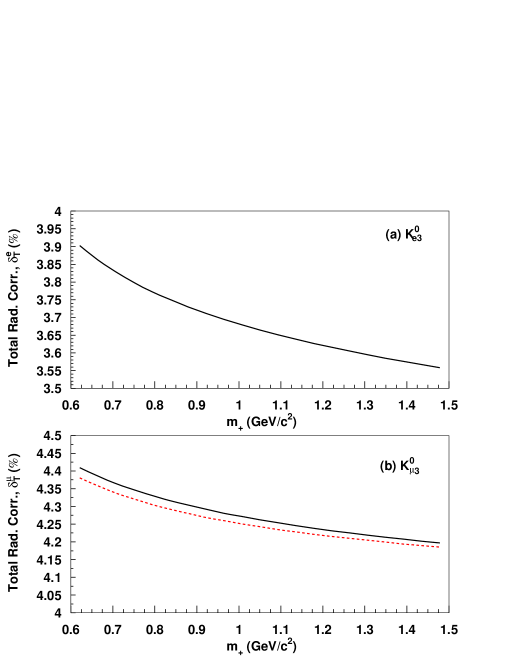
Figure 7: (a) Total radiative correction, $\delta^{e}_{T}$ ($=\delta^{e}_{LD}+\delta_{SD})$, to the $K^{0}_{e3}\$decay rate as a function of the $K^{*}$ pole mass $m_{+}$. Curve is generated using Method II and $m_{0}=1.174$ GeV/c². (b) Total radiative correction, $\delta^{\mu}_{T}$ ($=\delta^{\mu}_{LD}+\delta_{SD})$, to the $K^{0}_{e3}\$decay rate as a function of the $K^{*}$ pole mass $m_{+}$. Curves are generated using Method II and $m_{0}=1.174$ GeV/c² (solid) and $m_{0}=0.9$ GeV/c² (dashed).

Using the phenomenological model and a cutoff scale of $\Lambda=m_{p}$, we find that the long-distance radiative corrections to the $K^{0}_{e3}\$and the $K^{0}_{\mu 3}\$decay modes are $1.3\%$ and $1.9\%$, respectively. For this model, the uncertainties on $\delta^{e}_{LD}$  and $\delta^{\mu}_{LD}$  result from the cutoff scale/virtual calculation method ($0.3$%) and the form factor parameter dependence ($0.04$%). Therefore, we take the uncertainty on $\delta^{e}_{LD}$  and $\delta^{\mu}_{LD}$  to be $\sim 0.3\%$.

In previous studies of the long-distance radiative corrections, Refs. [20, 21] found that $\hat{\delta}^{e}_{LD}=1.5\%$ and $\hat{\delta}^{\mu}_{LD}=2.0\%$ [40]. Recall that $\hat{\delta}^{\ell}_{LD}$  ($\ell=e$, or $\mu$) corresponds to the long-distance radiative correction inside the $K^{0}_{\ell 3}\$three-body Dalitz regions. Since $\hat{\delta}^{\ell}_{LD}<\delta^{\ell}_{LD}$, one infers that $\delta^{e}_{LD}>1.5\%$ and $\delta^{\mu}_{LD}>2.0\%$ from Ref. [20, 21]. Using our calculation with a constant form factor model, $\delta^{e}_{LD}=1.3\%$ and $\delta^{\mu}_{LD}=1.9\%$ [see Table 1 and Table 2]. The cause of the discrepancy between the $\delta^{\ell}_{LD}$  values is unknown; however, Ref. [8] has noted a formerly undocumented error in the $K^{+}_{\ell 3}\$calculation of Ref. [20, 21]. Therefore, one possible explanation is an unknown error in the $K^{0}_{\ell 3}\$calculation of Ref. [20, 21].

A more recent study [8] of the $K^{0}_{e3}\$decay rate using   finds that for $\Lambda=m_{\rho}$, $\hat{\delta}^{e}_{LD}$  is $0.6\%$. When the cutoff scale is taken to be $m_{p}$, $\hat{\delta}^{e}_{LD}$  should increase by $\sim 0.1\%$. In our calculation, we find that for the $K^{0}_{\ell 3}\$decay rate, the contribution to $\delta^{e}_{LD}$  from outside the $K^{0}_{e3}\$Dalitz region is $\sim+0.5\%$. Therefore, we infer that $\delta^{e}_{LD}\sim 1.2\%$ from Ref. [8], which agrees with our calculation.

Predictions of the phenomenological model may be tested experimentally. One way to test the long-distance radiative corrections $\delta^{e}_{LD}$  and $\delta^{\mu}_{LD}$  is to test the ratio

$${\mathcal{F}}_{LD} = \frac{1+\delta^{\mu}_{LD}}{1+\delta^{e}_{LD}}.$$ (32)

Using our radiative correction parameters, we find that ${\mathcal{F}}_{LD}=1.0058\pm 0.001$. The uncertainty in ${\mathcal{F}}_{LD}$ is obtained from Table 1 and Table 2; note that the common cutoff scale uncertainties likely cancel in the ratio. Using Eq. (10) and assuming lepton universality, the ratio ${\mathcal{F}}_{LD}$ equals

$$\frac{\Gamma_{K^{0}_{\mu 3}\ }}{\Gamma_{K^{0}_{e3}\ }}\cdot\frac{I^{e}_{(0)}(\lambda_{i})}{I^{\mu}_{(0)}(\lambda_{i})},$$ (33)

where $\Gamma_{K^{0}_{\mu 3}\ }/\Gamma_{K^{0}_{e3}\ }$ is the ratio of the $K^{0}_{e3}\$and the $K^{0}_{\mu 3}\$decay rates, $I^{e}_{(0)}(\lambda_{i})/I^{\mu}_{(0)}(\lambda_{i})$ is the ratio of the lowest order $K^{0}_{e3}\$and $K^{0}_{\mu 3}\$phase space integrals [see Eq. (8)], and the $\lambda_{i}$ are form factor model parameters.

Using the measured decay rates and the form factors from Ref. [4], we find that the experimental value of ${\mathcal{F}}_{LD}$ is $1.0027\pm 0.0048$. This is consistent with our calculated value.

5.3 Radiative Fractions

In addition to the fraction ${\mathcal{F}}_{LD}$ defined in Eq. (32), the phenomenological model may be used to predict other experimentally-measurable quantities. In this section, we use the phenomenological model to predict the fraction of radiative events that satisfy requirements on the photon’s energy and angular distance from the charged lepton. Radiative fractions for $K^{0}_{\ell 3}\$decays were originally proposed by Ref. [23] and later refined in Refs. [7, 41].

The radiative fractions are defined by the equation

$${\mathcal{R}}^{0}_{K\ell 3}(E^{\rm\rm min}_{\gamma},\,\theta^{\rm min}_{\ell\gamma})=\Gamma(K^{0}\rightarrow\pi^{-}\ell^{+}\nu\gamma;\,E_{\gamma}\geq E^{\rm min}_{\gamma},\,\theta_{\ell\gamma}\geq\theta^{\rm min}_{\ell\gamma})/\Gamma_{K^{0}_{\ell 3}\ },$$ (34)

where $E^{\rm min}_{\gamma}$ is the minimum energy of the radiated photon, and $\theta^{\rm min}_{\ell\gamma}$ is the minimum angular separation between the photon and the charged lepton, and $\Gamma_{K^{0}_{\ell 3}\ }$ is the $K^{0}_{\ell 3}\$decay rate including radiative corrections. Both $E^{min}_{\gamma}$ and $\theta^{\rm min}_{\ell\gamma}$ are quantities defined in the kaon center of mass.

In Table 3, we present the calculated radiative fractions. For the $K^{0}_{e3}\$and the $K^{0}_{\mu 3}\$decay modes we consider two values of $E^{\rm min}_{\gamma}$: $10$ MeV and $30$ MeV. We do not make any requirement on the angular separation between the photon and the muon; however, for the $K^{0}_{e3}\$decay mode, we also consider $\theta^{\rm min}_{\ell\gamma}=20^{\circ}$. The uncertainties in Table 3 are composed of two components: the uncertainty on the next-to-leading order correction and the uncertainty on the $K^{0}_{\ell 3}\$decay rates. For the $K^{0}_{e3}\$and the $K^{0}_{\mu 3}\$decay modes, we take the uncertainty on the next-order corrections to be $1.3$% and $1.9$% of $\Gamma(K^{0}\rightarrow\pi^{-}\ell^{+}\nu\gamma;\,E_{\gamma}\geq E^{\rm min}_{\gamma},\,\theta_{\ell\gamma}\geq\theta^{\rm min}_{\ell\gamma})$, respectively. We estimate the uncertainties on the $K^{0}_{\ell 3}\$decay rate by using the $0.3\%$ uncertainty on the radiative correction parameters, $\delta^{\ell}_{LD}$.

Table 3: Radiative fraction, ${\mathcal{R}}^{0}_{K\ell 3}(E^{\rm min}_{\gamma},\,\theta^{\rm min}_{\ell\gamma})$, as defined in Eq. (34). Radiative fractions are given in percent(%) and they are presented for both the $K^{0}_{e3}\$and $K^{0}_{\mu 3}\$decay modes.

	${\mathcal{R}}^{0}_{Ke3}$ (%)		${\mathcal{R}}^{0}_{K\mu 3}$ (%)
$E^{\rm min}_{\gamma}$ / $\theta^{\rm min}_{\ell\gamma}$	$0^{\circ}$	$20^{\circ}$	$0^{\circ}$
$10$ MeV	$4.93\pm 0.06$	$1.89\pm 0.02$	$0.564\pm 0.01$
$30$ MeV	$2.36\pm 0.03$	$0.956\pm 0.01$	$0.214\pm 0.004$

6 Conclusions

We have studied radiative corrections to the $K^{0}_{e3}\$and the $K^{0}_{\mu 3}\$decay modes using a phenomenological model for their interactions. In our calculation, we include the contribution to the radiative correction from outside the three-body $K^{0}_{\ell 3}\$Dalitz region. Using the cutoff scale $\Lambda=m_{p}$, we find that $\delta^{e}_{LD}=(1.3\pm 0.3)\%$ and $\delta^{\mu}_{LD}=(1.9\pm 0.3)\%$. The uncertainty in the long-distance radiative corrections is dominated by their sensitivity to the cutoff scale $\Lambda$ and virtual calculation method. Dependence of the radiative corrections on the variation of the hadronic $K$–$\pi$ form factors is found to be small ($0.04\%$). The calculated value of the $\delta^{e}_{LD}$ radiative correction parameter agrees with a recent calculation [8] using .

Combining the long-distance contribution from the phenomenological model with the short-distance contribution from Ref. [17], the total radiative corrections to the $K^{0}_{e3}\$and the $K^{0}_{\mu 3}\$modes are $(3.5\pm 0.3)\%$ and $(4.1\pm 0.3)\%$. The uncertainty in the total radiative corrections are dominated by the uncertainty in the long-distance component. When measuring the $V_{us}$ CKM matrix element, the uncertainty from radiative corrections should be $\sim 0.0003$. This uncertainty corresponds to a small fraction of the “external uncertainty” ($0.0021$) quoted for the $|V_{us}|$ measurement in Ref. [4].

The program KLOR was written to numerically evaluate the radiative corrections and to generate Monte Carlo events. Monte Carlo events produced by KLOR may be used to understand experimental detection efficiencies.

Appendix A Loop Integrals

Virtual corrections to the $K^{0}_{\ell 3}\$decay mode require the evaluation of loop integrals. Below, we define the loop integrals for one-, two-, three-, and four- point functions [37, 38, 42]. The corresponding vector loop integrals and their expansion in terms of momentum four-vectors are also defined. In Sec. 5, we numerically evaluate the loop integrals using the cutoff regularization scheme. Therefore, implicit in our definition is a high-mass, cutoff scale, $\Lambda$.

The scalar one-point function is

$$A(m^{2})=\frac{1}{i\pi}\int d^{4}k\frac{1}{(k^{2}-m^{2})},$$ (35)

where $m$ is a mass parameter.

The scalar two-point function is

$$\begin{array}[]{l}B_{0}(p_{1}^{2};m_{0}^{2},m_{1}^{2})=\frac{1}{i\pi}\int\frac{d^{4}k}{(k^{2}-m_{0}^{2})((k+p_{1})^{2}-m_{1}^{2})},\end{array}$$ (36)

where $p_{1}^{\mu}$ is a four-momentum and $m_{i}$ ($i=1,2$) are mass parameters. The vector two-point function is

$$B_{\mu}(p_{1};m_{0}^{2},m_{1}^{2})=\frac{1}{i\pi}\int\frac{d^{4}k\,k_{\mu}}{(k^{2}-m_{0}^{2})((k+p_{1})^{2}-m_{1}^{2})}=p_{1,\mu}B_{1}(p_{1}^{2};m_{0}^{2},m_{1}^{2}),$$ (37)

where $B_{\mu}(p_{1};m_{0}^{2},m_{1}^{2})$ is proportional to $p_{1,\,\mu}$.

The scalar three-point function is

$$C_{0}(p_{1}^{2},s_{12},p_{2}^{2};m_{0}^{2},m_{1}^{2},m_{2}^{2})=\frac{1}{i\pi}\int\frac{d^{4}k}{(k^{2}-m_{0}^{2})((k+p_{1})^{2}-m_{1}^{2})((k+p_{2})^{2}-m_{2}^{2})}$$ (38)

where $s_{ij}=(p_{i}-p_{j})^{2}$ is the squared difference of two four-momenta. The vector three-point function is

$$C_{\mu}(p_{1},p_{2};m_{0}^{2},m_{1}^{2},m_{2}^{2}) = \frac{1}{i\pi}\int\frac{d^{4}kk_{\mu}}{(k^{2}-m_{0}^{2})((k+p_{1})^{2}-m_{1}^{2})((k+p_{2})^{2}-m_{2}^{2})}$$ (39)

$$= p_{1,\mu}C_{1}+p_{2,\mu}C_{2},$$

where $C_{i}=C_{i}(p_{1}^{2},s_{12},p_{2}^{2};m_{0}^{2},m_{1}^{2},m_{2}^{2})$.

The scalar four-point function is

$$\begin{array}[]{ll}\lx@intercol D_{0}(p_{1}^{2},s_{12},s_{23},p_{3}^{2},p_{2}^{2},s_{13};m_{0}^{2},m_{1}^{2},m_{2}^{2},m_{3}^{2})\hfil\lx@intercol\\ &=\frac{1}{i\pi}\int d^{4}k\,[(k^{2}-m_{0}^{2})((k+p_{1})^{2}-m_{1}^{2})]^{-1}\\ &\hskip 34.1433pt\times[((k+p_{2})^{2}-m_{2}^{2})((k+p_{3})^{2}-m_{3}^{2})]^{-1}\end{array}$$ (40)

and the vector four-point function is

$$\begin{array}[]{ll}\lx@intercol D_{\mu}(p_{1},p_{2},p_{3};m_{0}^{2},m_{1}^{2},m_{2}^{2},m_{3}^{2})\hfil\lx@intercol\\ &=\frac{1}{i\pi}\int d^{4}k\,k_{\mu}\,[(k^{2}-m_{0}^{2})((k+p_{1})^{2}-m_{1}^{2})]^{-1}\\ &\hskip 35.56593pt\times[((k+p_{2})^{2}-m_{2}^{2})((k+p_{3})^{2}-m_{3}^{2})]^{-1}\\ &=p_{1,\mu}D_{1}+p_{2,\mu}D_{2}+p_{3,\mu}D_{3},\end{array}$$ (41)

where $D_{i}=D_{i}(p_{1}^{2},s_{12},s_{23},p_{3}^{2},p_{2}^{2},s_{13};m_{0}^{2},m_{1}^{2},m_{2}^{2},m_{3}^{2})$.

Appendix B Method II Expressions

As in Method I, the matrix element for the virtual corrections using Method II may be written in the following form:

$${\mathcal{M}}^{\rm virt}_{\rm pole}=\frac{\alpha}{4\pi}\sqrt{2}G_{F}V_{us}f_{+}(0)~{}\bar{u}(p_{\nu})P_{R}\left[A_{pole}{p}\!\!\!/_{K}-B_{pole}{p}\!\!\!/_{\ell}\ \right]v(p_{\ell}),$$ (42)

where $A_{pole}$ and $B_{pole}$ are composed of loop integrals. In this section, we present the expressions for these parameters.

We break-up the expression for $A_{pole}$ and for $B_{pole}$ into five components,

$$A_{pole}=\sum_{i=1}^{5}A_{i} B_{pole}=\sum_{i=1}^{5}B_{i},$$ , (43)

where the ‘$1$’ component is from inter-particle photon exchange, the ‘$2$’ component is from the $\pi$ and $\ell$ wavefunction renormalizations, the ‘$3$’ component is from photon exchange between the effective vertex and the charged lepton, the ‘$4$’ component is from photon exchange between the effective vertex and the pion, and the ‘$5$’ component comes from emission and re-absorption of a photon by the effective vertex. Since single photon radiation from the effective vertex is small, we expect that $A_{5}$ and $B_{5}$ (double photon radiation) are negligible [43].

The expressions for the $A_{i}$ and the $B_{i}$ may be written, compactly, in terms of a handful of two-, three-, and four- point functions. We define $B_{i}^{(\pi)}=B_{i}(m^{2}_{\pi};m^{2}_{\pi},\lambda^{2})$ and $B_{i}^{(\ell)}=B_{i}(m^{2}_{\ell};m^{2}_{\ell},\lambda^{2})$ where $i=0,1$. We also define the two-point functions that depend on the pole masses $m_{+}$ and $m_{0}$,

$$\begin{array}[]{lcl}B_{0}^{(\sigma,\,A)}&=&B_{0}(t;\lambda^{2},m^{2}_{\sigma})\\ B_{0}^{(\sigma,\,B)}&=&B_{0}(t;m^{2}_{\pi},m^{2}_{\sigma}),\\ B_{0}^{(\sigma,\,C)}&=&B_{0}(m^{2}_{K};m^{2}_{\pi},m^{2}_{\sigma}),\end{array}$$ (44)

where $\sigma=+,\,0$. We define the following four-point functions:

$$\begin{array}[]{lcl}C_{i}^{(\sigma,\,A)}&=&C_{i}(m^{2}_{\pi},m^{2}_{K},t;\lambda^{2},m^{2}_{\pi},m^{2}_{\sigma})\\ C_{i}^{(\sigma,\,B)}&=&C_{i}(s_{\pi\ell},0,m^{2}_{K};m^{2}_{\pi},m^{2}_{\ell},m^{2}_{\sigma})\\ C_{i}^{(\sigma,\,C)}&=&C_{i}(m^{2}_{\ell},t,0;m^{2}_{\ell},\lambda^{2},m^{2}_{\sigma})\\ C_{i}^{(\sigma,\,D)}&=&C_{i}(m^{2}_{\pi},t,m^{2}_{K};m^{2}_{\pi},\lambda^{2},m^{2}_{\sigma}),\end{array}$$ (45)

where $s_{ij}=(p_{i}-p_{j})^{2}$, $i=0,1,2$ and $\sigma=+,\,0$. We define the following four-point functions:

$$\begin{array}[]{l}D_{i}^{(\sigma)}=D_{i}(m^{2}_{\pi},s_{\pi\ell},0,t,m^{2}_{\ell},m^{2}_{K};\lambda^{2},m^{2}_{\pi},m^{2}_{\ell},m_{\sigma}^{2}),\end{array}$$ (46)

where $s_{ij}=(p_{i}-p_{j})^{2}$, $i=0,1,2,3$ and $\sigma=+,\,0$.

Using the above definitions, $A_{1}$ and $B_{1}$ are

$$A_{1} = -2m^{2}_{+}C_{0}^{(+,\,A)}-2{\Delta C_{0}^{B}}-{\Delta C_{1}^{A}}+8m^{2}_{+}x_{\pi\ell}D_{0}^{(+)}-2\lambda^{2}{\Delta D_{0}}$$

$$+4m^{2}_{+}m^{2}_{\pi}D_{1}^{(+)}+4x_{\pi\ell}\,{\Delta D_{1}}+4m^{2}_{+}(m^{2}_{\ell}+2x_{\pi\ell})D_{2}^{(+)}-2m^{2}_{\ell}\,{\Delta D_{2}}$$

$$+4m^{2}_{+}(m^{2}_{K}-m^{2}_{\pi})D_{3}^{(+)}-2t\,{\Delta D_{3}},$$

$$B_{1} = -\left[\Delta C_{0}^{A}+\Delta C_{1}^{A}+\Delta C_{2}^{A}\right]-2\,{\Delta C_{0}^{B}}+[4x_{\pi\ell}-2\lambda^{2}]{\Delta D_{0}}+[4x_{\pi\ell}-2m^{2}_{\pi}]{\Delta D_{1}}$$ (47)

$$+ 4m^{2}_{+}s_{\pi\ell}\,D_{2}^{(+)}+[4x_{\pi\ell}-2m^{2}_{\ell}]{\Delta D_{2}}+4m^{2}_{+}m^{2}_{K}D_{3}^{(+)}+[4x_{\pi\ell}-2t]{\Delta D_{3}},$$

where

$$\begin{array}[]{lcl}\Delta C_{i}^{X}&=&m^{2}_{+}C_{i}^{(+,\,X)}+(m^{2}_{K}-m^{2}_{\pi})\left[C_{i}^{(+,\,X)}-C_{i}^{(0,\,X)}\right],\\ \Delta D_{i}&=&m^{2}_{+}D_{i}^{(+)}+(m^{2}_{K}-m^{2}_{\pi})\left[D_{i}^{(+)}-D_{i}^{(0)}\right],\end{array}$$ (48)

and $X=A,\,B$. The components $A_{2}$ and $B_{2}$ are expressed in terms of the wavefunction renormalization constants [see Eq. (25)],

$$\begin{array}[]{lcl}A_{2}=\hat{f}_{+}(t)\left(\frac{4\pi}{\alpha}\right)\left(\delta Z_{\pi}+\delta Z_{\ell}\right)&,&B_{2}=\hat{f}_{2}(t)\left(\frac{2\pi}{\alpha}\right)\left(\delta Z_{\pi}+\delta Z_{\ell}\right),\end{array}$$ (49)

where $t=(p_{K}-p_{\pi})^{2}$. The $A_{i}$ and $B_{i}$ components arising from photon emission from the vertex and absorption by either the pion or the lepton ($i=3,4$) are given by the equations

$$A_{3} = \;\hat{f}_{+}(t)\left[4m^{2}_{\ell}C_{0}^{(+,C)}-4tC_{1}^{(+,C)}\right]$$

$$B_{3} = \;\hat{f}_{+}(t)\left\{-2B_{0}^{(0,\,A)}+\frac{2}{m^{2}_{+}}{\Delta B_{0}^{(A)}}-8x_{K\nu}\left[C_{0}^{(+,\,C)}+C_{1}^{(+,\,C)}+C_{2}^{(+,\,C)}\right]\right.$$ (50)

$$- \left.2\,m^{2}_{\ell}\;\left[C_{0}^{(0,\,C)}-m_{+}^{-2}{\Delta C_{0}^{(C)}}\right]+2t\left[C_{1}^{(0,\,C)}-m_{+}^{-2}{\Delta C_{1}^{(C)}}\right]\right\}$$

$$+\hat{f}_{2}(t)\left\{2B_{0}^{(0,\,A)}-4B_{0}^{(\ell)}-2B_{1}^{(\ell)}+2m^{2}_{\ell}C_{0}^{(0,\,C)}-2tC_{1}^{(0,\,C)}\right\},$$

and

$$A_{4} = \;\hat{f}_{+}(t)\left\{4B_{0}^{(A)}-2B_{0}^{(C)}-2B_{0}^{(\pi)}-2\left[2(m^{2}_{K}-m^{2}_{\pi})-t+\lambda^{2}-m^{2}_{+}\right]C_{0}^{(+,\,D)}\right\}$$

$$+{\Delta C_{0}^{(D)}}-{\Delta C_{1}^{(D)}}-{\Delta C_{2}^{(D)}}$$

$$B_{4} = \;{\Delta C_{0}^{(D)}}-{\Delta C_{1}^{(D)}}+\hat{f}_{2}(t)\left\{2B_{0}^{(+,\,A)}+B_{0}^{(\pi)}-B_{0}^{(+,\,C)}\right.$$ (51)

$$\left.-\left[2(m^{2}_{K}-m^{2}_{\pi})-t+\lambda^{2}-m^{2}_{+}\right]C_{0}^{(+,\,D)}\right\}$$

$$+\frac{2}{m^{2}_{0}}\hat{f}_{0}(t)\left\{-m^{2}_{+}B_{0}^{(+,\,A)}+\Delta B_{0}^{(A)}+\frac{1}{2}m^{2}_{+}B_{0}^{(+,\,B)}-\frac{1}{2}\Delta B_{0}^{(B)}\right.$$

$$-\frac{1}{2}\left[2(m^{2}_{K}-m^{2}_{\pi})-t+\lambda^{2}\right]C_{0}^{(+,\,D)}$$

$$\left.+\frac{1}{2}\left[2(m^{2}_{K}-m^{2}_{\pi})-t+\lambda^{2}\right]{\Delta C_{0}^{(D)}}+m^{2}_{+}C_{0}^{(+,\,D)}-m^{2}_{0}C_{0}^{(0,\,D)}\right\}.$$

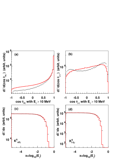
Figure 8: Comparison of the PHOTOS (dots) and the KLOR (line) Monte Carlo generators. (a) and (b) plot the cosine of the angle between the charged lepton and the photon ($\cos\theta_{\ell\gamma}$) for the $K^{0}_{e3}\$and the $K^{0}_{\mu 3}\$decay modes, respectively. In plots (a) and (b) radiated photons are required to have an energy greater than $10$ MeV in the kaon center of mass. Plots (c) and (d) compare the log of the radiated photon energy ($\log_{10}(E_{\gamma})$), where $E_{\gamma}$ is in GeV. In PHOTOS the IR cutoff is taken to be $1$ keV and in KLOR the photon mass was taken to be $1$ eV/c².

Appendix C Comparison of KLOR to PHOTOS

One tool often used by experimentalists to model radiative effects is a “universal” Monte Carlo generator called PHOTOS [10]. For the $K^{0}_{\ell 3}\$decay mode, PHOTOS estimates the size of the radiative corrections in the leading-logarithmic (collinear) approximation. Since it treats radiation from the charged lepton and the pion independently, PHOTOS should succeed in reproducing the photon energy distribution but fail to reproduce distributions of the angle between the photon and a charged particle. To illustrate this behavior, we generate the $\log(E_{\gamma})$ and the $\cos\theta_{\ell\gamma}$ distributions using PHOTOS and KLOR [see Fig. 8]. In $K^{0}_{e3}\$decays, PHOTOS significantly underestimates radiation in the central and backward directions, while for $K^{0}_{\mu 3}\$decays, photon radiation is suppressed in the central region. For both the $K^{0}_{e3}\$and $K^{0}_{\mu 3}\$decay modes, PHOTOS and KLOR agree for lower energy photons. The discrepancy at higher energies is most likely a result of the “soft photon” assumption in PHOTOS.

Though PHOTOS is a powerful tool, precision measurements of $K^{0}_{\ell 3}\$decays require a more accurate understanding of radiative effects. With KLOR, we hope to satisfy this requirement and be able to study the structure of the radiative corrections. It should be noted that the results of PHOTOS can be improved if the $K^{0}_{\ell 3}\$inner-bremsstrahlung matrix element is incorporated into the PHOTOS algorithm.

References

- [1] N. Cabibbo, Phys. Rev. Lett. 10 (1963) 531; M. Kobayashi and T. Maskawa, Prog. Theor. Phys. 49 (1973) 652.
- [2] S. Eidelman et al. [Particle Data Group], Phys. Lett. B 592 (2004) 1.
- [3] A. Sher et al., Phys. Rev. Lett. 91 (2003) 261802.
- [4] T. Alexopoulos et al. [KTeV Collaboration], Phys. Rev. Lett. 93 (2004) 181802.
- [5] T. Alexopoulos et al. [KTeV Collaboration], Phys. Rev. D 70 (2004) 092006.
- [6] T. Alexopoulos et al. [KTeV Collaboration], Phys. Rev. D 70 (2004) 092007.
- [7] L. Ametller, J. Bijnens, A. Bramon and F. Cornet, Phys. Lett. B 303, 140 (1993); J. Bijnens and P. Talavera, Nucl. Phys. B 669, 341 (2003).
- [8] V. Cirigliano, M. Knecht, H. Neufeld, H. Rupertsberger and P. Talavera, Eur. Phys. J. C 23 (2002) 121; V. Cirigliano, H. Neufeld and H. Pichl, Eur. Phys. J. C 35 (2004) 53.
- [9] V. Bytev, E. Kuraev, A. Baratt and J. Thompson, Eur. Phys. J. C 27 (2003) 57 [Erratum-ibid. C 34 (2004) 523].
- [10] Comput. Phys. Commun. 79 (1994) 291.
- [11] O. P. Yushchenko et al., Phys. Lett. B 589 (2004) 111.
- [12] A. Lai et al. [NA48 Collaboration], Phys. Lett. B 602 (2004) 41.
- [13] F. Ambrosino et al. [KLOE Collaboration], Phys. Lett. B 636 (2006) 166.
- [14] W. M. Yao et al. [Particle Data Group], J. Phys. G 33 (2006) 1.
- [15] C. Gatti, Eur. Phys. J. C 45, 417 (2006).
- [16] V. Cirigliano, presented at Flavor Physics and CP Violation (FPCP 2006), Vancouver, Canada, eConf C060409 (2006) 037.
- [17] W. J. Marciano and A. Sirlin, Phys. Rev. Lett. 71 (1993) 3629.
- [18] E. S. Ginsberg, Phys. Rev. 142 (1966) 1035.
- [19] E. S. Ginsberg, Phys. Rev. 162 (1967) 1570; 187 (1969) 2280E.
- [20] E. S. Ginsberg, Phys. Rev. 171 (1968) 1675; 174 (1968) 2169E; 187 (1969) 2280E.
- [21] E. S. Ginsberg, Phys. Rev. D 1 (1970) 229.
- [22] T. Becherrawy, Phys. Rev. D 1 (1970) 1452.
- [23] H. W. Fearing, E. Fischbach and J. Smith, Phys. Rev. D 2 (1970) 542.
- [24] E. Fischbach and J. Smith, Phys. Rev. 184 (1969) 1645.
- [25] L. M. Chounet, J. M. Gaillard and M. K. Gaillard, Phys. Rep. 4C (1972) 199.
- [26] Eq. (2) describes the semileptonic decay of the kaon mediated by a Standard Model boson (vector interaction). More general forms of the effective interaction allow for scalar and tensor form factors [25]. For a study of the effect of scalar and tensor interactions in decays, we refer the reader to Ref. [27]. Current experimental results on the potential size of exotic coupling in decays are found in Refs. [14, 28]. In this paper, we restrict our analysis to a model of decays consistent with the Standard Model.
- [27] M. V. Chizhov, Phys. Lett. B 381 (1996) 359.
- [28] R. J. Tesarek, hep-ex/9903069, talk given at American Physical Society (APS) Meeting of the Division of Particles and Fields (DPF 99), Los Angeles, CA, 5–9 Jan 1999.
- [29] J. J. Sakurai, Ann. Phys. (N.Y.) 11 (1960) 1; T. D. Lee, S. Weinberg, and B. Zumino, Phys. Rev. Lett. 18 (1967) 1029; T. D. Lee and B. Zumino, Phys. Rev. 163 (1967) 1667; J. Schwinger, Phys. Rev. Lett. 19 (1967) 1154.
- [30] H. Leutwyler and M. Roos, Z. Phys. C 25 (1984) 91.
- [31] The short- and long- distance corrections are often written separately using the and notation, respectively. The two formulations are related by the relation, , where .
- [32] F. E. Low, Phys. Rev. 110 (1958) 974.
- [33] T. H. Burnett and N. M. Kroll, Phys. Rev. Lett. 20 (1968) 86.
- [34] J. C. Ward, Phys. Rev. 78 (1960) 182.
- [35] G. P. Lepage, Journal of Comp. Phys. 27 (1978) 192.
- [36] W. H. Press, B. P. Flannery, S. A. Teukolsky, W. T. Vetterling, Numerical Recipes in Fortran (Cambridge University Press, Cambridge, 1992).
- [37] T. Hahn and M. Perez-Victoria, Comput. Phys. Commun. 118 (1999) 153.
- [38] G. J. Oldenborgh and J. A. M. Vermaseren, Z. Phys. C 46 (1990) 425.
- [39] Numerical values for are obtained by using Eq. (10) in Ref. [17]. Eq. (10) sums the leading short-distance logs but does not include the QCD factor . Therefore, the calculated values of quoted in Table 1 and Table 2 should be accurate to within .
- [40] The formulae for the radiative correction in Ref. [20, 21] are known to have errors that affect the results. The expressions have been updated in two subsequent errata. The numerical values of the long-distance radiative corrections, and , are from the second errata of Ref. [20].
- [41] M. G. Doncel, Phys. Lett. 32B (1970) 623.
- [42] G. ’t Hooft and M. J. G. Veltman, Nucl. Phys. B153 (1979) 365.
- [43] To calculate the effective vertex for double-photon radiation one may proceed in an analogous manner to the single-photon radiation case. Modulo structure-dependent terms, this vertex may be specified by requiring the Ward Identity to be satisfied: is zero when either or .