Cronin effect and high–$p_{\perp}$ suppression from the
Color Glass Condensate

Abstract

I give a pedagogical survey of the nuclear collective effects associated with gluon saturation and their impact on particle production in high–energy proton (or deuteron)–nucleus collisions at RHIC. At central rapidity, the theory predicts a Cronin peak due to independent multiple scattering off the valence quarks in the nucleus. At forward rapidities, the peak flattens out and disappears very fast, because of the correlations induced through quantum evolution in the nuclear gluon distribution at small $x$. Also, the ratio ${R}_{\rm pA}$ between the particle yield in proton–nucleus and proton–proton collisions is rapidly suppressed when increasing the rapidity, because of saturation effects which slow down the evolution of the nucleus compared to that of the proton. This behaviour could be responsible for a similar trend observed in the deuteron–nucleus collisions at RHIC.

1 I. Introduction

When accelerated up to RHIC energies ($\sim 100$ GeV/nucleon), a heavy ion such as a gold nucleus is expected to ‘evolve’ into a high–density form of hadronic matter — the “Color Glass Condensate” (CGC) MV ; CGC ; CGCreviews — whose properties are qualitatively different from those of ‘ordinary’ partonic systems at lower energies. This is the matter made of the small–$x$, ‘saturated’, gluons, and is characterized by an intrinsic momentum scale, the saturation momentum $Q_{s}$ GLR , which rises rapidly with the energy and the atomic number $A$ ($Q_{s}^{2}(x,A)\sim x^{-\lambda}A^{\delta}$ with $\lambda\sim 0.3$ and $\delta\sim 1/3$) and acts as an infrared cutoff in momentum integrals involving the gluonic spectrum (see CGCreviews for recent reviews). As usual, the variable $x$ denotes the longitudinal momentum fraction of the ‘interesting’ gluons — those which participate in the scattering —, and decreases rapidly when increasing the energy of the collision. Thus, for sufficiently small $x$ and/or large $A$, $Q_{s}(x,A)$ is a hard scale ($Q_{s}^{2}\gg\Lambda^{2}_{\rm QCD}$), which allows us to rely on perturbative techniques to get insight into the properties of the CGC and of the high energy scattering in QCD.

Of course, the CGC remains ‘virtual’ (it is a part of the nuclear wavefunction) before any scattering takes place, but one expects it to be ‘liberated’ in a high–energy nucleus–nucleus (or proton–nucleus) collision, and thus to determine the properties of the partonic system which is created immediately after the collision CGCreviews ; GM04 . This system must be strongly interacting (because of its high energy density and the many intervening degrees of freedom), and also highly off–equilibrium (in particular, because of the strong anisotropy in the initial distribution of energy and momentum), so it is expected to undergo a violent evolution, characterized in the early stages by a rapid longitudinal expansion and a redistribution of the energy, momentum and other quantum number among the various modes, possibly leading to a thermalized state (the “Quark–Gluon Plasma”) at intermediate stages GM04 , which then further expands and cools down, until it hadronizes into a multitude of hadrons (a few thousands) that are eventually captured by the detectors at RHIC QM02 ; QM04 . It appears therefore as a challenge for the theorists to imagine observables which could survive (almost) unchanged to such a violent evolution, and thus carry out information about the initial conditions (in particular, about the color glass). It is furthermore a challenge for the experimentalists to extract and measure such observables with a significant accuracy.

One of the observables which look most promising for a study of the initial conditions (since less sensitive to ‘final state interactions’) is the total multiplicity of produced particles

$$\frac{{\rm d}N}{{\rm d}\eta}\,=\,\int{\rm d}^{2}p_{\perp}\,\,\frac{{\rm d}N}{{\rm d}^{2}p_{\perp}{\rm d}\eta}\,,$$ (1)

where ${\rm d}N/{{\rm d}^{2}p_{\perp}{\rm d}\eta}$ denotes the spectrum of the produced hadrons (of a given species, or summed over several species), $p_{\perp}$ is the hadron transverse momentum, and $\eta$ is its (pseudo)rapidity :

$$\eta\,\equiv\,\frac{1}{2}\,\ln\,\frac{p+p_{z}}{p-p_{z}}\,=\,\frac{1}{2}\,\ln\,\frac{1+\cos\theta}{1-\cos\theta}\,=\,-\,\ln\,\tan\,\frac{\theta}{2}\,,$$ (2)

with $p=\sqrt{p_{\perp}^{2}+p_{z}^{2}}$ and $\theta$ the angle between the direction of the produced hadron and the collision axis. It is an experimental fact that the integral in Eq. (1) is dominated by small momenta. In fact, in lowest order perturbation theory, the spectrum diverges at small $p_{\perp}$ like $1/p_{\perp}^{4}$, and the corresponding integral is ill defined. But the non–linear effects encoded in the CGC — which, from the point of view of perturbation theory, correspond to all–orders resummations of high parton density effects — provide an infrared cutoff in the form of the saturation momentum $Q_{s}$, which at RHIC is estimated as $Q_{s}\sim$ 1 GeV. Note that this is marginally a hard scale, which justifies a posteriori the use of perturbation theory in the construction of the theory for the CGC CGCreviews .

One sees that the very calculability of the total multiplicity at RHIC within perturbative QCD is an indirect evidence for the saturation physics leading to the CGC. Note that, implicit in these considerations, is the assumption that the spectrum of the produced hadrons (as measured in the experiment) can be identified with the spectrum of the partons (mostly gluons) liberated in the early stages of the collisions (as computed in the CGC). This ‘duality’ hypothesis is far from being rigorous, but it has some theoretical motivation, and, more importantly, it seems to be roughly consistent with the data in various experimental settings. With this assumption, the CGC prediction for the total multiplicity ${\rm d}N/{{\rm d}\eta}$ at RHIC Raju turns out to be quite close to the actual value measured in the experiments. In fact, simple calculations within the CGC framework satisfactorily describe the global features of the total multiplicity at RHIC, like its dependencies upon the energy $\sqrt{s}$ and the rapidity $\eta$, and also upon the centrality of the collision (or the “number of participants”) KNL .

Another interesting prediction of the CGC theory that will be discussed at length in what follows refers to the interplay between the energy dependence and the nuclear ($A$) dependence of the gluon spectrum (by which I mean either the unintegrated gluon distribution in the nuclear wavefunction, or the spectrum of the gluons produced in a heavy ion collision, and which is further assimilated with the spectrum ${\rm d}N/{{\rm d}^{2}p_{\perp}\!{\rm d}\eta}$ of the produced hadrons). Because of coherence effects associated with the non–linear gluon dynamics, the gluon distribution of a large nucleus is not simply the incoherent sum of the corresponding distributions produced by $A$ separated nucleons. This is true not only in the saturation region at low momenta $p_{\perp}\mathrel{\hbox to0.0pt{\raise 2.20013pt\hbox{$<$}\hss}{\lower 2.20013pt\hbox{$\sim$}}}Q_{s}$ (where, as we shall see, the gluon distribution scales roughly like $A^{2/3}$ rather than like $A$), but also for momenta well above $Q_{s}$, where however the trend of the $A$–dependence depends upon $y$ and gets reversed when increasing the energy : Whereas at low energies, the theory MV ; K96 ; JKMW97 ; KM98 predicts an enhancement of the $A$–dependence due to ‘higher–twist’ rescattering effects (which fall off rapidly with increasing $p_{\perp}$; see Sect. III below), on the other hand, at sufficiently large energies, the quantum evolution of the color glass CGC considerably modifies the dominant, leading–twist, contribution (this acquires an ‘anomalous dimension’ GLR ; SCALING ; MT02 ; DT02 ), and thus provides a power–like suppression of the $A$–dependence, which persists up to relatively high $p_{\perp}$ SCALING (see also Sect. IV). This suppression is further amplified by running coupling effects AM03 .

This change of behaviour has dramatic consequences for the spectrum of the produced gluons (or hadrons): At low energies, one expects an enhancement at intermediate $p_{\perp}$ (“Cronin peak”) in the properly normalized production cross–section GJ02 ; JNV , while at higher energies, one should rather find a depletion within a wide range of momenta (“high–$p_{\perp}$ suppression”) KLM02 ; KKT ; Baier03 ; Nestor03 .

When the latter feature has been conceptually first realized KLM02 , the “high–$p_{\perp}$ suppression” was freshly discovered at RHIC QM02 — the high–$p_{\perp}$ yield in gold–gold collisions was found to be almost an order of magnitude lower than expected from jet production arising from incoherent parton–parton scattering d'Enterria —, so it was tempting to propose this “quantum saturation” scenario as a possible explanation of the data KLM02 . To further substantiate this scenario, it is worth mentioning that the onset of the anomalous dimension is closely related to another important prediction of the CGC, namely a new scaling law for the gluon distribution SCALING ; MT02 ; DT02 ; MP03 , which seems to be confirmed by the recent discovery of “geometric scaling” in the HERA data at small $x\leq 10^{-2}$ geometric . But in the context of Au+Au collisions at RHIC, the argument in Ref. KLM02 suffers from a serious drawback: A central–rapidity ($\eta=0$) jet with $p_{\perp}=5-10$ GeV is produced by partons with $x\sim 10^{-1}$, which is a too large value of $x$ for the quantum evolution of the CGC to play any role! Besides, the observed high–$p_{\perp}$ suppression can be also understood as arising from a completely different physical mechanism: energy loss through final–state interactions (or ‘jet quenching’) JetQuenching .

Nowadays, we know that this last explanation is in fact the correct one. The decisive evidence in that sense came from another set of experiments at RHIC in which one of the two heavy nuclei beams has been substituted by a deuteron beam, thus eliminating the final–state interactions. Fig.  1 exhibits the experimental results obtained by PHENIX and STAR for the nuclear modification factor in deuteron–gold collisions $(R_{\rm dAu})$ compared to gold–gold $(R_{\rm AuAu})$. (BRAHMS and PHOBOS have reported similar results; see Refs. in RHIC-dAu-mid .) Here, for generic nuclei A and B which scatter with impact parameter $b_{\perp}$, the ratio $R_{\rm AB}$ is defined as:

$$R_{\rm AB}(\eta,p_{\perp},b_{\perp})\,\equiv\,\frac{1}{\langle N_{\rm coll}(b)\rangle}\,\frac{{\rm d}N_{\rm A+B}/{\rm d}\eta{\rm d}^{2}p_{\perp}{\rm d}^{2}b_{\perp}}{{\rm d}N_{\rm p+p}/{\rm d}\eta{\rm d}^{2}p_{\perp}{\rm d}^{2}b_{\perp}}\,,$$ (3)

where ${\langle N_{\rm coll}(b_{\perp})\rangle}$ denotes the average number of collisions for a centrality bin at the given impact parameter. This definition is such that $R_{\rm AB}$ would be equal to one if A+B were an incoherent superposition of nucleon–nucleon collisions; converserly, its deviation from one is a measure of collective nuclear effects.

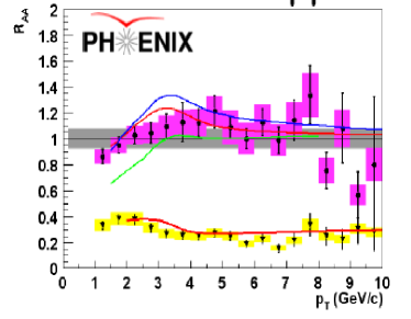
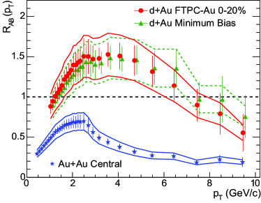
Figure 1: Central rapidity ($\eta=0$) PHENIX $\pi^{0}$ and STAR $h^{\pm}$ data comparing $R_{\rm dAu}$ to $R_{\rm AuAu}$  RHIC-dAu-mid . These results, together with similar data from BRAHMS and PHOBOS RHIC-dAu-mid , prove that jet quenching in Au+Au collisions at central rapidity is necessarily a final state effect.

The data in Fig.  1 clearly show enhancement (rather than suppression) in the $R_{\rm dAu}$ ratio at moderately large $p_{\perp}$. As already mentioned, and will be detailed in Sect. III, this Cronin peak can be attributed to the multiple interactions suffered by the colliding parton from the deuteron on its way through the nucleus (see Fig.  2).

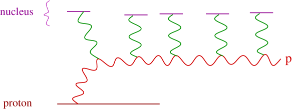
Figure 2: Multiple scattering in a proton–nucleus collision. In the experiments at RHIC, the proton is actually replaced by a deuteron.

The parton scatters off gluons with a relatively large momentum fraction $x\sim 0.1$, but whose density is still quite large (hence the importance of multiple scattering), because the gold nucleus contains many color sources already at low energy: the $3A\sim 600$ valence quarks. The results in Fig.  1 demonstrate that the strong suppression (by a factor 4 to 5) observed in $R_{\rm AuAu}$ cannot be attributed to the quantum evolution of the gluon distribution in the nuclear wavefunction (otherwise, a similar effect would be seen at $\eta=0$ also in $R_{\rm dAu}$), and thus indirectly confirm its origin as a final–state effect.

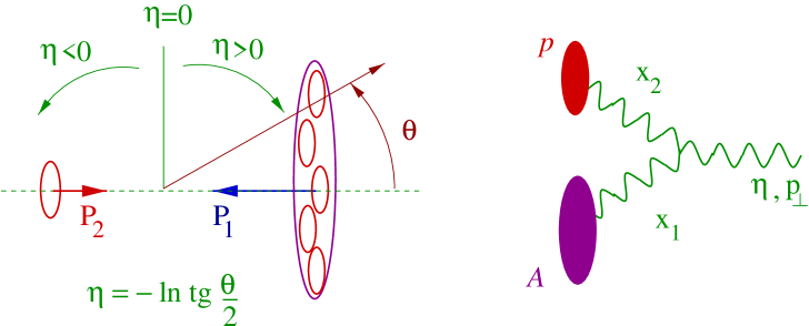
Figure 3: Kinematics for gluon production via gluon fusion in proton($p$)–nucleus($A$) collisions (d+Au collisions are similar). With light–cone notations [$k^{\mu}=(k^{+},k^{-},{\bf k}_{\perp})$, with $k^{\pm}=(E_{k}\pm k_{z})/\sqrt{2}$], the nucleons involved in the collision have purely longitudinal momenta: $P^{\mu}_{1}=(0,P_{1},0_{\perp})$ and $P^{\mu}_{2}=(P_{2},0,0_{\perp})$, with $P_{1}=P_{2}=\sqrt{s/2}$ in the center-of-mass frame, while the emerging gluon has $p^{\mu}=\Big{(}\frac{p_{\perp}}{\sqrt{2}}\,{\rm e}^{\eta},\frac{p_{\perp}}{\sqrt{2}}\,{\rm e}^{-\eta},{\bf p}_{\perp}\Big{)}$. Energy–momentum conservation implies $x_{1}\equiv{k_{1}^{-}}/{P_{1}}=({p_{\perp}}/{\sqrt{s}})\,{\rm e}^{-\eta}$ and $x_{2}\equiv{k_{2}^{+}}/{P_{2}}=(p_{\perp}/{\sqrt{s}})\,{\rm e}^{\eta}$, where $k_{1,2}$ refer to the two gluons which fuse with each other. Thus, larger positive values for $\eta$ correspond to smaller values for the longitudinal fraction $x_{1}$ of the gluon from the nucleus.

More recently, the BRAHMS experiment has presented the first results for $R_{\rm dAu}$ at ‘forward rapidities’ ($\eta=2-3$ in the deuteron fragmentation region; see Fig. 3) Brahms-data , which have been soon after confirmed by the other collaborations QM04 . The most remarkable feature about these new data is that they show a strong dependence upon $\eta$, and also a general trend with both $\eta$ and the centrality which at a first sight looks counterintuitive and surprising: As argued before, the Cronin enhancement is attributed to multiple scatterings between a parton from the deuteron and the gluons in the nucleus. When increasing $\eta$, we are probing gluons with smaller values of $x$ (see kinematics in the capture to Fig. 3), so the gluon distribution must increase, and this should favour the rescattering effects and thus enhance the Cronin peak. Similarly, more central collisions are probing regions with higher density, which should again enhance the Cronin peak. But the experimental results show precisely the opposite trends (cf. Fig.  5) !

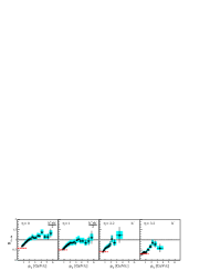
Figure 4: BRAHMS results for d+Au collisions at 200 GeV/nucleon Brahms-data : The ratio $R_{\rm dAu}$ for charged hadrons as a function of $p_{\perp}$ for central and forward pseudorapidities.

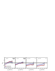
Figure 5: d+Au collisions at BRAHMS Brahms-data : The ratio $R_{\rm CP}$ of yields from collisions of a given centrality class (0-20% or 30-50%) to yields from more peripheral collisions (60-80%), scaled by the mean number of binary collisions in each sample, as a function of $p_{\perp}$ for central and forward pseudorapidities.

But as counterintuitive as it might seem, this behaviour has been in fact anticipated, on the basis of the CGC ideas KLM02 ; KKT ; Nestor03 : As already mentioned, one effect of the quantum evolution towards smaller values of $x$ is to suppress the dependence of the high–$p_{\perp}$ spectrum upon the atomic number $A$, or, more generally, upon the number of colliding particles in a given centrality bin. What came nevertheless as a surprise is the fact that this suppression sets in so fast ! As manifest on Fig.  5, the centrality dependence gets reversed already for $\eta=2$ (which corresponds to $x\sim 10^{-3}$ for $p_{\perp}=4$ GeV), while for $\eta=3.2$ ($x\sim 5\times 10^{-4}$), the data in Fig.  4 show suppression ($R_{\rm dAu}<1$) at all the measured values of $p_{\perp}$.

In fact, already before the advent of the BRAHMS data, the rapid evolution of the ratio $R_{\rm AB}$ with increasing $\eta$ has been observed theoretically Nestor03 , in a numerical calculation based on the Balitsky–Kovchegov (BK) equation B ; K . In Ref. Nestor03 , the Cronin peak was seen to flatten out and completely disappear after only one unit of rapidity. But the mechanism responsible for such a rapid evolution has been fully elucidated only subsequently, through an exhaustive analytic study IIT04 , which has also clarified other important issues like the respective roles of the proton and the nucleus in the evolution with $\eta$, and the effects of the running of the coupling. The main results of this study will be briefly described in the remaining part of this review.

2 II. The ${R}_{\rm pA}$–ratio in the CGC

For simplicity, in what follows I shall discuss proton($p$)+nucleus($A$) scattering, and assume that similar results hold also for the d+Au collisions of interest at RHIC. The physically interesting quantity is then the ratio (compare to Eq. (3))

$$R_{\rm pA}(\eta,p_{\perp})\,\equiv\,\frac{1}{A^{1/3}}\,\frac{\frac{{\rm d}N_{\rm pA}}{{\rm d}\eta{\rm d}^{2}p_{\perp}{\rm d}^{2}b_{\perp}}}{\frac{{\rm d}N_{\rm pp}}{{\rm d}\eta{\rm d}^{2}p_{\perp}{\rm d}^{2}b_{\perp}}}\,,$$ (4)

between the yield of produced gluons per unit phase–space (i.e., per unit of pseudorapidity, transverse momentum and impact parameter) in $pA$ and $pp$ collisions normalized by $A^{1/3}$ (since, at a fixed impact parameter, the number of nucleons available for scattering in a $pA$ collision is larger by a factor $A^{1/3}$ than in the corresponding $pp$ collision; note that I assume homogeneity in impact parameter space, for simplicity). Thus, the ratio (4) measures the difference between $pp$ collisions and an incoherent superposition of proton–nucleon collisions, and is an useful observable to pinpoint collective effects like gluon saturation in the wavefunction of the incoming nucleus .

So, how to compute gluon production in $pA$ collisions ? Leaving aside the fully numerical calculations Raju ; JNV (and Refs. therein) based on the classical version of the CGC theory (the McLerran–Venugopalan model MV ; CGCreviews ; see also Sect. III below), which apply to both $pA$ and $AA$ collisions but have not been extended yet to include the quantum evolution with $\eta$, all (semi)analytic calculations of the ${R}_{\rm pA}$–ratio KLM02 ; KKT ; Baier03 ; Nestor03 ; IIT04 rely on the factorization of the cross–section for particle production in terms of the gluon distributions in the target and the projectile (“$k_{T}$–factorization”), which has been since long proven for $pp$ collisions (see, e.g., FR ), and has been shown in the recent years to also hold for $pA$ collisions KM98 ; DM01 ; KT02 ; BGV04 , provided a special definition is used for the nuclear gluon distribution Braun which incorporates rescattering effects.

Up to an irrelevant normalization factor which cancels out in the ratio (4), the gluon yield in $pA$ collisions can be computed as (see kinematics in Fig. 3)

$$\frac{{\rm d}N_{\rm pA}}{{\rm d}\eta{\rm d}^{2}p_{\perp}{\rm d}^{2}b_{\perp}}\,\propto\,\frac{1}{p_{\perp}^{2}}\int d^{2}k_{\perp}\,\varphi_{A}(k_{\perp},y_{1})\,\varphi_{p}(p_{\perp}-k_{\perp},y_{2})\,,$$ (5)

where $y$ denotes the gluon rapidity, related to its longitudinal momentum fraction $x$ via $y=\ln(1/x)$, and $\varphi_{A}(k_{\perp},y)$ is the gluon occupation factor , i.e., the number of gluons of given spin and color per unit phase–space in a nucleus with atomic number $A$:

$$\varphi_{A}(k_{\perp},y)\,\equiv\,\frac{(2\pi)^{3}}{2(N_{c}^{2}-1)}\,\,\frac{{\rm d}N^{\rm gluon}_{A}}{{\rm d}y\,{\rm d}^{2}k_{\perp}{\rm d}^{2}b_{\perp}}\,.$$ (6)

($N_{c}=3$ is the number of ‘colors’.) For $pp$ collisions, a similar formula holds with $\varphi_{A}(k_{\perp},y_{1})$ replaced by $\varphi_{p}(k_{\perp},y_{1})$. Note that $y_{1,2}=y_{0}\pm\eta$, with $y_{0}\equiv\ln({\sqrt{s}}/k_{\perp})$ (cf. Fig. 3). Thus increasing $\eta$ amounts to increasing $y_{1}$ but decreasing $y_{2}$.

Clearly, the nuclear effects enter the previous formulae via the nuclear gluon distribution $\varphi_{A}$ : Unlike its proton counterpart $\varphi_{p}$, which is the standard, leading–twist, ‘unintegrated gluon distribution’ generally used in conjunction with $k_{T}$–factorization FR , $\varphi_{A}$ encodes higher–twist effect associated with the rescattering suffered by the gluon partaking in the collision while it crosses the nucleus.

At central pseudo–rapidity ($\eta=0$) and for the high–$p_{\perp}$ kinematics at RHIC, $y_{1}=y_{0}$ is rather small, so one can assume that the gluons in the nuclear distribution $\varphi_{A}(k_{\perp},y_{1})$ are produced by direct radiation from the valence quarks. In that case, Eq. (5) describes the multiple scattering between a gluon in the proton and the valence quarks in the nucleus, as illustrated in Fig. 2. The effect of the rescattering on the ratio ${R}_{\rm pA}$ will be discussed in the next section, within the context of a simple model for the distribution of the valence quarks, introduced by McLerran and Venugopalan MV .

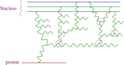
Figure 6: $pA$ collision at forward rapidity: the (relatively large–$x$) gluon emitted by the incoming proton scatters off the highly–evolved gluon distribution in the nuclear wavefunction at small–$x$. Non–linear effects (which correspond to either gluon recombination in the nuclear wavefunction, or multiple scattering of the ‘external’ gluon) are indicated by small cercles.

At forward, and sufficiently large, pseudo–rapidities ($\eta=2-3$), the gluons with $y_{1}=y_{0}+\eta$ in the nuclear wavefunction are predominantly produced by quantum evolution from lower values of $y_{1}$ BFKL , that is, they are emitted by gluons with larger values of $x$ which are themselves radiated by the valence quarks. Since the gluon density was rather large to start with (due to the large number of valence quarks), and it is further amplified by the evolution with $\eta$, the newly emitted gluons propagate in a strong background field — the color field created by sources (valence quarks or gluons) at larger values of $x$ — and undergo multiple scattering off the latter (see Fig. 6). This rescattering introduces a negative feedback (it reduces the number of gluons), and eventually leads to gluon saturation. Computing $\varphi_{A}$ in this non–linear regime requires an analysis of the quantum evolution in the presence of strong fields, which has been completed only recently CGC ; B ; K ; JKLW97 ; W ; SAT ; AM01 ; SCALING ; MT02 , with results to be discussed in Sect. IV.

The simplify the discussion while keeping all the salient physical features, it is convenient to replace the ratio in Eqs. (4)–(5) by the simpler quantity

$${\mathcal{R}}_{pA}(k_{\perp},y)\,\equiv\,\frac{\varphi_{A}(k_{\perp},y)}{A^{1/3}\,\varphi_{p}(k_{\perp},y)}\,,$$ (7)

to be considered for $y=y_{2}$, i.e., for the rapidity of the gluon in the nuclear wavefunction which participates in the collision. Eq. (7) measures the difference between the gluon distribution in the nucleus and that in the proton (scaled up by $A^{1/3}$) at the same (small) value of $x$, and thus is the most direct expression of the nuclear effects which should be responsible for the deviation of the experimentally measured ratio ${R}_{\rm pA}$ from one. In particular, qualitative effects like the Cronin enhancement or the high–$p_{\perp}$ suppression should be already visible (and theoretically easier to study) on the ratio (7); this is confirmed by the analyses in Refs. KKT ; Nestor03 , which have found a similar qualitative behaviour for the quantities defined in Eqs. (4)–(5) and, respectively, Eq. (7). In what follows I shall exclusively focus on the simpler ratio, Eq. (7).

3 III. Central rapidity: Cronin peak in the MV model

So long as the rapidity $y$ is not too large, one can ignore quantum evolution towards small $x$ and describe the gluon distribution in the nucleus as the result of classical radiation from the valence quarks. This is probably a good approximation for particle production in d+Au collisions at central rapidity ($\eta=0$), since in that case $y=y_{0}\sim 3$ is still quite small. (From experience with the phenomenology at HERA, we expect small–$x$ evolution effects to become important only for $y>5$, corresponding to $x<10^{-2}$ ; see e.g. IIM03 and references therein.)

The gluon spectrum ${\rm d}N_{A}/{\rm d}y\,{\rm d}^{2}k_{\perp}{\rm d}^{2}b_{\perp}$ is produced by the valence quarks located within a tube of transverse area $\sim 1/k_{\perp}^{2}$ which traverses the nucleus in longitudinal direction at impact parameter $b_{\perp}$ (so the length of the tube scales like $A^{1/3}$). If the transverse section of this tube is much smaller than the area of a single nucleon (i.e., $k_{\perp}^{2}\gg\Lambda_{\rm QCD}^{2}$), then the valence quarks which are included inside the tube belong typically to different nucleons. It is then reasonable to assume, following McLerran and Venugopalan MV , that these quarks are uncorrelated with each other. But although the color charges of these quarks sum up incoherently, this is generally not so for the corresponding gluon distributions (unlike it would happen for photon distributions in QED), because the classical color fields obey a non–linear equation: the Yang–Mills equation.

It is convenient to consider first the case of a proton, since there the color fields are still weak, and one can rely on the linear approximation. Then, the total gluon distribution is simply the incoherent sum of the distributions produced by the $N_{c}=3$ valence quarks, which by themselves can be evaluated with the well known formula for bremsstrahlung:

$$\frac{{\rm d}N_{\rm quark}}{{\rm d}y\,{\rm d}^{2}k_{\perp}}\,=\,\frac{\alpha_{s}C_{F}}{\pi^{2}}\,\frac{1}{k_{\perp}^{2}}\,.\qquad\quad(C_{F}=(N_{c}^{2}-1)/2N_{c})$$ (8)

After multiplying this by $N_{c}$ and dividing the result by the number of (gluonic) color states $N_{c}^{2}-1$ and by the proton area $\pi R^{2}_{p}$, one finds the occupation factor as (cf. Eq. (6)):

$$\varphi_{A}(k_{\perp})\,\simeq\,\frac{\mu_{p}}{k_{\perp}^{2}}\,,\qquad\mu_{p}\,\equiv\,\frac{2\alpha_{s}}{R^{2}_{p}}\,.$$ (9)

Physically, $\mu_{p}$ is the color charge squared of the valence quarks per unit transverse area (here, in the proton). Eq. (9) is valid for $k_{\perp}\gg Q_{p}$ with $Q_{p}\sim\Lambda_{\rm QCD}$ a non–perturbative scale related to confinement.

Moving to a large nucleus, one finds $\mu_{A}\simeq A^{1/3}\mu_{p}$, but the calculation of the corresponding gluon distribution is more elaborate, as it requires the exact solution to the Yang–Mills equation with a strong color source. This has been solved indeed, with the following result JKMW97 ; K96 ; KM98 ; CGCreviews :

$$\varphi_{A}(k_{\perp})\,=\,\!\int\!d^{2}r_{\perp}\,{\rm e}^{-ik_{\perp}\cdot r_{\perp}}\,\,\frac{1-{\rm exp}\Big{\{}-\frac{1}{4}\,\alpha_{s}N_{c}r_{\perp}^{2}\mu_{A}\ln{4\over r_{\perp}^{2}\Lambda^{2}}\Big{\}}}{\pi\alpha_{s}N_{c}r_{\perp}^{2}}\,,\,\,$$ (10)

where $\Lambda\sim\Lambda_{\rm QCD}$ is a non–perturbative scale introduced by hand to cut off an infrared divergence which physically should be removed by confinement. This formula features the saturation momentum $Q_{s}(A)$, defined by

$$Q_{s}^{2}(A)\,=\,\alpha_{s}N_{c}\mu_{A}\,\ln\frac{Q_{s}^{2}(A)}{\Lambda^{2}}\,\,\sim\,A^{1/3}\,\ln A^{1/3}\,,$$ (11)

(note that when $r=2/Q_{s}(A)$ the exponent in Eq. (10) is equal to one), as the intrinsic transverse momentum scale which separates the linear regime from the non–linear one:

(i) At high momenta $k_{\perp}\gg Q_{s}(A)$, one can expand the exponential in Eq. (10), and thus obtain (I only show here the first two terms in this expansion) :

$$\varphi_{A}(k_{\perp})\,\simeq\,\frac{\mu_{A}}{k_{\perp}^{2}}\,+\,\alpha_{s}N_{c}\left(\frac{\mu_{A}}{k_{\perp}^{2}}\right)^{2}\left[\ln\frac{k_{\perp}^{2}}{\Lambda^{2}}+2\gamma-2\right],\qquad{\rm for\quad}k_{\perp}\gg Q_{s}(A)\,.$$ (12)

The first term, which gives the dominant behaviour at high $k_{\perp}$, is recognized as the bremsstrahlung spectrum, corresponding to independent emissions from the valence quarks. This is as expected: At high momenta, non–linear effects become negligible because the corresponding modes have only little overlap with each other. Thus, for sufficiently high momenta, $\varphi_{A}(k_{\perp})\,\simeq\,A^{1/3}\varphi_{p}(k_{\perp})$, and the ratio ${\mathcal{R}}_{pA}(k_{\perp})$ approaches one from the above.

(ii) At low momenta $k_{\perp}\ll Q_{s}(A)$ (with $k_{\perp}\gg\Lambda$ though), the dominant behavior is obtained after neglecting the exponential term in Eq. (10), and reads

$$\varphi_{A}(k_{\perp})\,\simeq\,\frac{1}{\alpha_{s}N_{c}}\,\left\{\ln\frac{Q_{s}^{2}(A)}{k_{\perp}^{2}}\,+\,\mathcal{O}\big{(}1\big{)}\right\}\,,\qquad{\rm for\quad}k_{\perp}\ll Q_{s}(A)\,.$$ (13)

This is parametrically large, $\mathcal{O}\big{(}1/\alpha_{s})$, but increases only slowly (logarithmically) when decreasing $k_{\perp}$ and/or increasing the atomic number $A$. This behaviour, which should be contrasted with the corresponding power–law behaviour (in both $1/k_{\perp}^{2}$ and $A$) of Eq. (12), is the hallmark of gluon saturation (here, within the MV model).

Because of this change in behaviour, the ratio (7) becomes very small at low momenta $k_{\perp}\ll Q_{s}(A)$ (where it is proportional to $k_{\perp}^{2}$), but it increases rapidly with $z\equiv k_{\perp}^{2}/Q_{s}^{2}(A)$, and becomes parametrically large (and, in particular, larger than one) for momenta in the vicinity of the nuclear saturation momentum. Indeed, for $z\sim 1$, $\varphi_{A}\sim 1/\alpha_{s}N_{c}$ and $\varphi_{p}\sim\mu_{p}/Q_{s}^{2}(A)$ (cf. Eq. (9)), and by also using $\mu_{A}=A^{1/3}\mu_{p}$, one finds

$${\mathcal{R}}_{pA}(k_{\perp})\,\sim\,\rho_{A}\,>\,1\,\qquad{\rm for\quad}k_{\perp}\sim Q_{s}(A)\,,$$ (14)

where (cf. Eq. (11)) :

$$\rho_{A}\,\equiv\,\frac{Q_{s}^{2}(A)}{\alpha_{s}N_{c}\mu_{A}}\,=\,\ln\frac{Q_{s}^{2}(A)}{\Lambda^{2}}\,\sim\ln A^{1/3}\,.$$ (15)

The estimate (14) holds up to corrections of $\mathcal{O}(1)$, which are indeed suppressed in the limit of a very large nucleus, for which $\rho_{A}\gg 1$. To make contact with RHIC phenomenology, it is useful to notice that, for a gold nucleus at RHIC energies, one expects $Q_{s}^{2}(A)\simeq 2$ GeV² GM04 , which together with $\Lambda\simeq 200$ MeV implies $\rho_{A}\simeq\ln 50\simeq 4$.

The previous considerations show that the ration ${\mathcal{R}}_{pA}$ must have a maximum as a function of $k_{\perp}$, with the position of the maximum near $Q_{s}(A)$ and the height of the peak of $\mathcal{O}\big{(}\ln A^{1/3}\big{)}$. This is confirmed by an exact (analytic) calculation IIT04 of the nuclear gluon spectrum in the MV model, Eq. (10), which together with Eq. (9) for the corresponding spectrum in the proton leads to the ratio ${\mathcal{R}}_{pA}$ displayed in Fig. 7 (the left figure there). The location $z_{0}$ of the maximum and its height ${\mathcal{R}}_{\rm max}(A)\equiv{\mathcal{R}}_{pA}(z_{0})$ can be computed analytically, in an expansion in powers of $1/\rho_{A}$ IIT04 :

$$z_{0}\,=\,0.435\,+\,\frac{0.882}{\rho_{A}}\,+\,{\mathcal{O}}\big{(}\rho_{A}^{-2}\big{)},\qquad{\mathcal{R}}_{\rm max}(A)\,=\,0.281\,\rho_{A}\,+\,0.300\,+\,{\mathcal{O}}\big{(}\rho_{A}^{-1}\big{)}\,.$$ (16)

In Fig. 7, it is also shown the result of a calculation including running coupling effects in the MV model (the right figure there). This is obtained by simply replacing the explicit factors of $\alpha_{s}$ in Eq. (10) by the one–loop running coupling : $\alpha_{s}\rightarrow\alpha_{s}(4/r_{\perp}^{2})$, with $\alpha_{s}(Q^{2})\equiv b_{0}/\ln(Q^{2}/\Lambda_{\rm QCD}^{2})$. Then, the scale which plays the role of a saturation momentum reads simply $Q^{2}_{s}(A)\equiv b_{0}N_{c}\mu_{A}$, and scales like $A^{1/3}$. In that case too, the gluon distribution in the MV model can be computed analytically IIT04 , and the results are rather similar (at least, qualitatively) to the fixed coupling case. In particular, the parameter $\rho_{A}\equiv\ln{Q_{s}^{2}(A)}/{\Lambda^{2}}$ plays again an important role — with a running coupling, this appears even more naturally, as the inverse of the running coupling: $\rho_{A}=b_{0}/\alpha_{s}(Q^{2}_{s}(A))$ —, and expansions like those in Eq. (16) can be again derived. (It turns out that the coefficients of the dominant terms in these expansions — for both $z_{0}$ and ${\mathcal{R}}_{\rm max}(A)$ — are the same for fixed and running coupling.)

The plots in Fig. 7 not only confirm that a maximum exists, but also show that this maximum is rather well pronounced, which could not have been anticipated solely on the basis of the previous approximations, Eqs. (12) and (13). To understand that, one needs also the behaviour of the nuclear gluon spectrum $\varphi_{A}(k_{\perp})$ for momenta around $Q_{s}(A)$. The calculations in Refs. IIT04 ; Adrian reveal that, when increasing $k_{\perp}$ above $Q_{s}(A)$, $\varphi_{A}(k_{\perp})$ starts by decreasing exponentially with $z=k^{2}/Q_{s}^{2}(A)$, before eventually relaxing, for $z>\ln\rho_{A}$, to the power law decay displayed in Eq. (12). To better illustrate this, Fig. 7 exhibits also the individual contributions to $\mathcal{R}_{pA}$ denoted as $\mathcal{R}^{\rm sat}_{pA}$ and $\mathcal{R}^{\rm twist}_{pA}$ which are obtained after separating $\varphi_{A}(k_{\perp})$ into two pieces: the ‘twist’ piece $\varphi_{A}^{\rm twist}$, which resums all the terms which at high–momenta decay as inverse powers of $z$ (the first two terms in this series are shown in Eq. (12)), and the ‘saturating’ piece $\varphi_{A}^{\rm sat}\equiv\varphi_{A}-\varphi_{A}^{\rm twist}$, which at $z\ll 1$ has the logarithmic behaviour shown in Eq. (13), whereas for $z>1$ decays exponentially with $z$. For any $z\mathrel{\hbox to0.0pt{\raise 2.20013pt\hbox{$<$}\hss}{\lower 2.20013pt\hbox{$\sim$}}}\ln\rho_{A}$, the saturating piece dominates over the twist piece, and thus $\mathcal{R}_{pA}$ has a rapid fall off at momenta just above the maximum (within the range $1\mathrel{\hbox to0.0pt{\raise 2.20013pt\hbox{$<$}\hss}{\lower 2.20013pt\hbox{$\sim$}}}z\mathrel{\hbox to0.0pt{\raise 2.20013pt\hbox{$<$}\hss}{\lower 2.20013pt\hbox{$\sim$}}}\ln\rho_{A}$), leading to the well–pronounced Cronin peak manifest in Fig. 7.

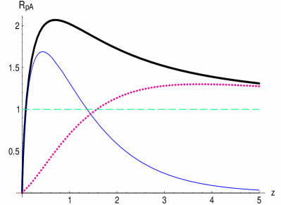
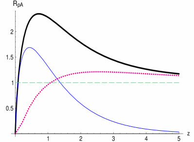
Figure 7: The ratio $\mathcal{R}_{pA}(z)$ as a function of the scaled momentum variable $z=k^{2}/Q_{s}^{2}(A)$ in the fixed (left) and running (right) coupling McLerran-Venugopalan model for $\rho_{A}=6$. The thick line corresponds the ratio $\mathcal{R}_{pA}(z)$; the solid line shows the saturation contribution $\mathcal{R}^{\rm sat}_{pA}(z)$; the dotted line shows the twist contribution $\mathcal{R}^{\rm twist}_{pA}(z)$. (From Ref. IIT04 .)

To conclude this discussion, let me comment on the physical origin of the Cronin enhancement in this classical model for saturation. As already mentioned in the Introduction, the Cronin peak is generally associated with multiple scattering within the nucleus (cf. Fig.  2). This is also the case in the present context, except for the fact that, since we are looking directly at the wavefunction (rather than at a scattering process), the multiple scattering is replaced by non–linear effects in the production of virtual gluons from the valence quarks. (One can say that, after one gluon is produced by some quark, it scatters off the color fields produced by the other quarks.) Since the gluon mutual interactions are repulsive, and are stronger at low momenta, their net effect is to rearrange the gluon distribution in transverse momentum space KKT ; IIT04 : Whereas in the bremsstrahlung spectrum $\propto 1/k_{\perp}^{2}$ most quanta are located at low momenta, in the presence of non–linear effects, the would–be low–$k_{\perp}$ gluons are pushed towards higher momenta, in such a way to minimize their repulsion. Some of these ‘displaced’ gluons are responsible for the ‘higher–twist’ contributions to the tail of the distribution at $k_{\perp}\gg Q_{s}(A)$ (cf. Eq. (12)). But most of them are quasi–uniformly redistributed at lower momenta $\mathrel{\hbox to0.0pt{\raise 2.20013pt\hbox{$<$}\hss}{\lower 2.20013pt\hbox{$\sim$}}}Q_{s}(A)$, thus giving a saturation plateau at $k_{\perp}\leq Q_{s}(A)$ (cf. Eq. (13)) IIT04 .

4 IV. Non–linear gluon evolution in the CGC

The non–linear evolution of the gluon distribution with increasing $y=\ln 1/x$ is described by the renormalization group equation for the CGC, also known as the JIMWLK equation CGC ; JKLW97 ; W , which is a functional (or operator) equation, that is, it generates an infinite hierarchy of ordinary integro–differential equations which couple the evolution of various $n$–point functions. These equations resum those radiative corrections which are enhanced by either the large rapidity gap (namely, the terms of order $(\alpha_{s}y)^{n}$ for any $n\geq 1$), or the high gluon density (since, e.g., the gluon occupation factor being of $\mathcal{O}\big{(}1/\alpha_{s})$ at saturation, it interferes with the perturbative expansion). This complicated evolution is illustrated in Fig. 6 which shows a typical gluon cascade which develops in the nuclear wavefunction at small $x$. The horizontal rungs in this cascade are radiated gluons which are strongly ordered in rapidity, while the mergings between various vertical branches, as well as the multiple scattering of the produced gluon, are representative for the non–linear effects in this high–energy environment. The general solution to the JIMWLK equation is not known, but approximate solutions have been constructed which separately cover the non–linear regime deeply at saturation, $k_{\perp}\ll Q_{s}(A,y)$, (where remarkable simplifications occur in the evolution equations, due to saturation SAT ), and the linear regime at $k_{\perp}\gg Q_{s}(A,y)$, where the gluon occupation factor $\varphi_{A}(k_{\perp},y)$ obeys a closed, linear, equation: the BFKL equation BFKL .

Remarkably, it turns out that the gluon occupation factor deeply at saturation ($k_{\perp}\ll Q_{s}(A,y)$) has the same simple form as in the classical MV model (cf. Eq. (13)), namely,

$$\varphi_{A}(k_{\perp},y)\,\approx\,\frac{1}{\alpha_{s}N_{c}}\,\left\{\ln\frac{Q_{s}^{2}(A,y)}{k_{\perp}^{2}}\,+\,\mathcal{O}\big{(}1\big{)}\right\}\,,\qquad{\rm for\quad}k_{\perp}\ll Q_{s}(y,A)\,,$$ (17)

where the saturation momentum is exponentially increasing with $y$ GLR :

$$Q_{s}^{2}(A,y)\,\simeq\,Q_{s}^{2}(A)\,{\rm e}^{c\bar{\alpha}_{s}y}\,,\qquad{\rm(fixed\,\,coupling)},$$ (18)

where $c\simeq\,4.88$ and $\bar{\alpha}_{s}\equiv\alpha_{s}N_{c}/\pi$. In this and the subsequent formulae, the variable $y$ denotes the difference from the rapidity $y_{0}$ corresponding to $\eta=0$; that is, from now on, $y$ is numerically the same as the pseudo–rapidity $\eta$.

Note the special way how Eq. (17) depends upon $A$, $y$ and $k_{\perp}$ : $\varphi_{A}(k_{\perp},y)$ is solely a function of the dimensionless ratio $z\equiv k_{\perp}^{2}/Q_{s}^{2}(A,y)$. This property, known as geometric scaling geometric , reflects the fact that $Q_{s}(A,y)$ is the only intrinsic scale at saturation.

Another remarkable feature is that geometric scaling is approximately preserved within a wide range of momenta above $Q_{s}$, where the evolution is linear SCALING . One finds indeed that, within the range

$$Q_{s}(A,y)\,\ll\,k_{\perp}\,\ll\,Q_{s}^{2}(A,y)/Q_{s}(A)\qquad{\rm(`extended\,\,scaling\,\,window^{\prime})},$$ (19)

the solution to the BFKL equation with saturation boundary conditions at $k_{\perp}\sim Q_{s}$ is well approximated by the scaling form SCALING ; MT02 ; MP03 :

$$\varphi_{A}(k_{\perp},y)\approx\frac{1}{\alpha_{s}N_{c}}\,\left\{\ln\frac{k_{\perp}^{2}}{Q_{s}^{2}(A,y)}\,+\,\mathcal{O}\big{(}1\big{)}\right\}\left(\frac{Q_{s}^{2}(A,y)}{k_{\perp}^{2}}\right)^{\gamma},\qquad\gamma\approx 0.63.$$ (20)

The difference $1-\gamma\approx 0.37$ is sometimes referred to as an ‘anomalous dimension’. Indeed, the fact that $\gamma$ is strictly smaller than one makes the function in Eq. (20) to show weaker dependencies upon $A$ and $1/k_{\perp}^{2}$ than the leading twist approximation (that one could naively expect to apply at momenta above $Q_{s}$). Below, I shall succinctly refer to the window (19) as the ‘BFKL regime’.

The standard leading twist (or DGLAP) approximation is recovered only at even higher momenta $k_{\perp}\gg Q_{s}^{2}(A,y)/Q_{s}(A)$, where the gluon occupation factor is extremely small, and the only trace of saturation is visible in the fact that it is the original saturation momentum at $y=0$, i.e., $Q_{s}(A)$, which acts as the infrared cutoff for the transverse phase–space available for evolution. Namely, because of the collinear singularity of QCD (see, e.g., Eq. (8)), the phase–space for the emission of a single (high–$k_{\perp}$) gluon is ${\rm d}k_{\perp}^{2}/k_{\perp}^{2}$, and therefore the total phase–space available for the evolution from $Q_{s}(A)$ up to $k_{\perp}$ is $\rho(A,k_{\perp})\equiv\ln k_{\perp}^{2}/Q_{s}^{2}(A)$. Within the present approximations, the solution to the linear equation which resums such small–$x$ and collinear gluon emissions is given by

$$\varphi_{A}(k_{\perp},y)\,\simeq\,\frac{\mu_{A}}{k_{\perp}^{2}}\,\,{\rm exp}\left\{\sqrt{4\bar{\alpha}_{s}y\rho(A,k_{\perp})}\right\}\,,$$ (21)

which is recognized as the evolution of the leading–twist term in the classical distribution (the first term in the r.h.s. of Eq. (12)). Eq. (21) is known as the “double–logarithmic accuracy”, or DLA, approximation, and is strictly valid so long as $\bar{\alpha}_{s}y\rho\gg 1$.

By using the previous formulae, together with similar formulae for the proton, it is possible to compute the ratio $\mathcal{R}_{pA}(k_{\perp},y)$ and follow its evolution with $y$. The corresponding formulae for the case of a running coupling $\alpha_{s}\equiv\alpha_{s}(k_{\perp}^{2})$ are quite similar (at least, within the kinematical ranges in which Eqs. (17) and (20) apply, i.e., at saturation and in the BFKL regime), with one crucial difference though: the functional form of the saturation momentum, which for running coupling reads SCALING ; MT02 ; AM03

$$Q_{s}^{2}(A,y)\,\simeq\,\Lambda^{2}_{\rm QCD}\,\,{\rm exp}\left\{\sqrt{2cby+\rho_{A}^{2}}\right\}\,,$$ (22)

where $b\equiv{12N_{c}}/{(11N_{c}-2N_{f})}$ and $c\simeq\,4.88$ is the same number as in Eq. (18). As compared to the corresponding formula for a fixed coupling, Eq. (18), the expression (22) shows a less rapid increase with $y$ at high energies, and also a weaker dependence upon the atomic number $A$, which becomes less important with increasing $y$ AM03 :

$$\frac{Q_{s}^{2}(A,y)}{Q_{s}^{2}(p,y)}\,\simeq\,\,\exp\left\{\frac{\rho_{A}^{2}-\rho_{p}^{2}}{2\sqrt{2cby}}\right\}\,\qquad{\rm for}\qquad 2cby\,\gg\,\rho_{A}^{2}\,>\,\rho_{p}^{2}\,,$$ (23)

and eventually disappears:

$$Q_{s}^{2}(A,y)\,\simeq\,\Lambda^{2}_{\rm QCD}\,{\rm e}^{\sqrt{2cby}}\,\qquad{\rm for}\qquad 2cby\,\gg\,\rho_{A}^{4}\,.$$ (24)

For sufficiently large energies, quantum evolution with running coupling washes out completely the difference between a nucleus and a proton !

5 V.  Forward rapidities: High–$p_{\perp}$ suppression

We are now prepared for a study of the evolution of the ratio $\mathcal{R}_{pA}(k_{\perp},y)$ with increasing $y$, starting with the initial condition provided by the MV model (which exhibits Cronin enhancement at intermediate momenta, as discussed in Sect. III).

5.1 V.1.  Quantum evolution of $\mathcal{R}_{pA}$ : General features

Let me first summarize the main features of the evolution, and then develop some of them in the next subsections:

a) The main effect of the evolution is a rapid suppression of the ratio $\mathcal{R}_{pA}$, due to the different evolution rates for the gluon distributions in the nucleus (the numerator in Eq. (7)) and in the proton (the denominator there). The proton distribution grows faster because, for the same values of $k_{\perp}$ and $y$, the transverse phase–space available for its evolution is larger than that for the nucleus. Indeed, as noticed in Sect. IV, the transverse phase–space $\int^{k_{\perp}}\big{(}{\rm d}^{2}p_{\perp}/p_{\perp}^{2}\big{)}$ is limited by the infrared cutoff introduced by the initial conditions at $y=0$. For the nucleus, this cutoff is the relatively hard scale $Q_{s}(A)$ associated with saturation ; thus, the nuclear phase–space $\rho(A,k_{\perp})\equiv\ln k_{\perp}^{2}/Q_{s}^{2}(A)$ is considerably smaller than the proton one, $\rho(p,k_{\perp})\equiv\ln k_{\perp}^{2}/Q_{p}^{2}$ with $Q_{p}\sim\Lambda_{\rm QCD}$. Specifically,

$$\rho(p,k_{\perp})\,\equiv\,\ln\frac{k_{\perp}^{2}}{Q_{p}^{2}}\,=\,\ln\frac{k_{\perp}^{2}}{Q_{s}^{2}(A)}+\ln\frac{Q_{s}^{2}(A)}{Q_{p}^{2}}\,\simeq\,\rho(A,k_{\perp})+\rho_{A},$$ (25)

where $\rho_{A}\gg 1$ has been generated according to Eq. (15). Correspondingly, ${\mathcal{R}}_{pA}(k_{\perp},y)$ decreases very fast with $y$, and already after a short evolution $y\sim 1/(\bar{\alpha}_{s}\rho_{A})\,\sim 1$ it becomes smaller than one at all but the asymptotic momenta.

b) By the same argument, the suppression goes away at extremely large momenta, where the difference between $Q_{s}(A)$ and $Q_{p}$ becomes unimportant in computing the phase–space. In fact, when $k_{\perp}\gg Q_{s}(A,y)$, one can use the DLA formula (21) for both the proton and the nucleus, and thus deduce (for fixed coupling) :

$${\mathcal{R}}_{pA}(k_{\perp},y)\,\simeq\,{\rm e}^{-\rho_{A}\sqrt{Y/\rho(A,k_{\perp})}}\qquad{\rm for}\qquad k_{\perp}\gg Q_{s}(A,y)\,,$$ (26)

which approaches one from below when $k_{\perp}\to\infty$.

c) The suppression rate $\,{\rm d}\ln{\mathcal{R}}_{pA}/{\rm d}y\,$ is largest at small $y\,$ and for not so large transverse momenta [say, for $\,k_{\perp}\mathrel{\hbox to0.0pt{\raise 2.20013pt\hbox{$<$}\hss}{\lower 2.20013pt\hbox{$\sim$}}}Q_{s}^{2}(A,y)/Q_{s}(A)\,$], since in this regime the dissymmetry between the evolution of the proton and that of the nucleus is most pronounced: The proton is in the DLA regime, and thus evolves very fast (because of the large transverse phase–space available to it), whereas the nucleus shows geometric scaling, and evolves only slowly (because, so long as $\bar{\alpha}_{s}y<1$, the nuclear saturation momentum rises very little; see Eq. (18)).

This explains, in particular, the rapid suppression in ${\mathcal{R}}_{pA}$ observed in the early stages of the evolution in the numerical study in Ref. Nestor03 .

d) For larger $y$ such that $\bar{\alpha}_{s}y\mathrel{\hbox to0.0pt{\raise 2.20013pt\hbox{$>$}\hss}{\lower 2.20013pt\hbox{$\sim$}}}1$, the ratio ${\mathcal{R}}_{pA}(k_{\perp},y)$ is monotonously increasing with $k_{\perp}$. That is, the Cronin peak has flattened out during the first $1/\bar{\alpha}_{s}$ units of rapidity.

e) The flattening of the Cronin peak cannot be attributed to the proton evolution alone — the latter produces a quasi–uniform suppression in ${\mathcal{R}}_{pA}$ at momenta around $Q_{s}(A,y)$, so, by itself, it would preserve a local structure like a peak—, rather this must be related to the evolution of the nucleus. As we shall see, it is indeed the nuclear evolution which washes out that distinguished feature of the initial distribution which was responsible for the existence of a well–pronounced peak at $y=0$ : the exponential fall off of the gluon occupation factor at momenta just above the saturation plateau (cf. Sect. III).

f) Whereas the generic features of the evolution, as described above, are qualitatively similar for both fixed and running coupling, important differences persist between these two scenarios as far as the details of the evolution, and also the precise structure of the final results, are concerned. Specifically, after including running coupling effects, the evolution appears to be slower (one needs a larger increase in rapidity to achieve a given suppression in $\mathcal{R}_{pA}$), but eventually stronger (the final value for $\mathcal{R}_{pA}$ which is obtained after a very large evolution in $y$ is significantly smaller with running coupling than with fixed coupling). Let me be more specific on these two points:

To appreciate how fast is the evolution, let me introduce the rapidity $y_{0}$ after which the ratio ${\mathcal{R}}_{pA}(k_{\perp},y)$ at $k_{\perp}\sim Q_{s}(A,y)$ decreases from its initial value of ${\mathcal{O}}(\rho_{A})$ (cf. Eq. (14)) to a value of ${\mathcal{O}}(1)$. In the next subsection, we shall see that

$$y_{0}\,\simeq\,\frac{1}{4\bar{\alpha}_{s}}\,\frac{\ln^{2}\rho_{A}}{\rho_{A}}\,\sim\,\frac{\big{(}\ln\ln A^{1/3}\big{)}^{2}}{\ln A^{1/3}}\,\qquad{\rm(fixed\,\,coupling)}\,,$$ (27)

(which incidentally is a very small rapidity interval: $\bar{\alpha}_{s}y_{0}\ll 1$), and, respectively,

$$y_{0}\,\simeq\,\frac{1}{4b}\,\ln\rho_{A}\,\sim\,\ln A^{1/3}\qquad{\rm(running\,\,coupling)},$$ (28)

which for large $A$ is parametrically larger than the fixed coupling estimate in Eq. (27); thus, the running of the coupling slows down the evolution.

Furthermore, to characterize the strength of the suppression after a very large rapidity evolution, consider the limit of ${\mathcal{R}}_{pA}$ when $y\to\infty$ with fixed $z\equiv k_{\perp}^{2}/Q_{s}^{2}(A,y)$. (This is the meaningful way to take the large–$y$ limit, since the interesting physics is located around the nuclear saturation momentum.) For $z={\mathcal{O}}(1)$, one finds:

$${\mathcal{R}}_{pA}(z\sim 1,y\to\infty)\,\sim\,\frac{1}{(A^{1/3}\rho_{A})^{1-\gamma}}\,\qquad{\rm(fixed\,\,coupling)}\,,$$ (29)

and, respectively,

$${\mathcal{R}}_{pA}(z\sim 1,y\to\infty)\,=\,\frac{1}{A^{1/{3}}}\,\,\qquad{\rm(running\,\,coupling)}\,.$$ (30)

As anticipated, for large $A$, the running coupling result (30) is much smaller than the corresponding one for fixed coupling, Eq. (29) (recall that $1-\gamma\simeq 0.37$).

In fact, the power of $A^{1/3}$ in the r.h.s. of Eq. (30) is simply the factor introduced by hand in the definition (7) of ${\mathcal{R}}_{pA}$. That is, the result (30) arises directly from the observation that, with a running coupling and for sufficiently large $y$, the nuclear and proton saturation scales coincide with each other, cf. Eq. (24), so the corresponding occupation factors will coincide as well, in the whole kinematic range for geometric scaling (which includes the saturation domain at $z\leq 1$ and the BFKL regime (19)).

g) The dependence of the ratio ${\mathcal{R}}_{pA}$ upon $A$ is also interesting, since this corresponds to the centrality dependence of the ratio $R_{\rm dAu}$ measured at RHIC Brahms-data ; QM04 . Consider the $A$–dependence for momenta around the Cronin peak: Whereas at $y=0$, the ratio ${\mathcal{R}}_{pA}(k_{\perp}\sim Q_{s}(A))$ is logarithmically increasing with $A$ (recall Eq. (14)), this tendency is rapidly reversed by the evolution (see the next subsection) : After only a small rapidity increase $y\sim 1/(\bar{\alpha}_{s}\rho_{A})\,\sim 1$, ${\mathcal{R}}_{pA}(k_{\perp},y)$ becomes a decreasing function of $A$ for any $k_{\perp}$, in qualitative agreement with the corresponding change in the centrality dependence observed in the data, cf. Fig. 5.

5.2 V.2. The suppression of the Cronin peak

I shall now use some simple calculations to illustrate the prominent role played by the proton evolution for the suppression of ${\mathcal{R}}_{pA}$ (especially at small $y$). For definiteness, I shall consider the fixed coupling case and focus on transverse momenta of the order of the nuclear saturation momentum, since this is the region where the Cronin peak is located at $y=0$. (The generalization of the discussion below to a running coupling and to arbitrary transverse momenta can be found in Ref. IIT04 .) So, let’s consider the evolution with $y$ of the following quantity (the ratio (7) along the nuclear saturation line) :

$${\mathcal{R}}_{\rm sat}(A,y)\equiv{\mathcal{R}}_{pA}(k_{\perp}=Q_{s}(A,y),y)\,.$$ (31)

Along this line, the nuclear gluon distribution reduces to a constant, due to geometric scaling (cf. Eq. (17)) :

$$\varphi_{A}(k_{\perp}=Q_{s}(A,y),y)\sim 1/{\alpha_{s}N_{c}}\,.$$ (32)

As for the corresponding distribution in the proton, this is given by the linear (BFKL) evolution, since $k_{\perp}=Q_{s}(A,y)\gg Q_{s}(p,y)$. Specifically, for relatively small $y$, such that $\bar{\alpha}_{s}y\ll\rho_{A}$, the evolution is dominated by the large transverse logarithm $\rho(p,k_{\perp})\sim\rho_{A}$ (cf. Eq. (25)), and the proton is described by the DLA formula (21), while for $\bar{\alpha}_{s}y\mathrel{\hbox to0.0pt{\raise 2.20013pt\hbox{$>$}\hss}{\lower 2.20013pt\hbox{$\sim$}}}\rho_{A}$ the proton enters the BFKL regime, where Eq. (20) applies. The ‘critical’ rapidity $\bar{\alpha}_{s}y_{c}\sim\rho_{A}$ at which the proton changes from DLA to BFKL is the upper limit for the geometric scaling window (19), now applied to the proton.

I) $\bar{\alpha}_{s}y\ll\rho_{A}$ : The early stages of the evolution (proton at DLA)

Using Eq. (21) with $A\to p$ and $k_{\perp}=Q_{s}(A,y)$, together with $\rho(p,Q_{s}(A,y))\simeq\rho_{A}$ (cf. Eq. (25)) and the definition (15), one immediately finds:

$${\mathcal{R}}_{\rm sat}(A,y)\,\,\sim\,\rho_{A}\,\,{\rm exp}\Big{\{}c\bar{\alpha}_{s}y-\sqrt{4\bar{\alpha}_{s}y\rho_{A}}\,\Big{\}}.$$ (33)

For $y=0$, this is parametrically large, ${\mathcal{R}}_{\rm sat}(A,y=0)\sim\rho_{A}$, as expected (cf. Eq. (14)). But when increasing $y$ (with $\bar{\alpha}_{s}y\ll\rho_{A}$ though), the ratio decreases very fast — the DGLAP increase of the proton distribution being faster than the BFKL increase of the nuclear saturation momentum, cf. Eq. (18) —, and becomes parametrically of $\mathcal{O}(1)$ already after the very short rapidity evolution

$$\bar{\alpha}_{s}y_{0}\,\sim\,\frac{\ln^{2}\rho_{A}}{4\rho_{A}}\,\,\ll\,1\,,$$ (34)

which is Eq. (27). This value $y_{0}$ is so small that one can in fact ignore the corresponding evolution of the nucleus: The rapid decrease in the height of the peak in the very early stages of the evolution is entirely due to the DGLAP evolution of the proton.

In fact, Eq. (33) shows that, larger is $\rho_{A}$ (i.e., higher was the original peak at $y=0$), faster is the suppression seen when increasing $y$ (i.e., smaller is $y_{0}$). This is so since $\rho_{A}$ also fixes the transverse phase–space for the DGLAP evolution of the proton, and as such it enters the exponential factor in Eq. (33). For the same reason, the ratio (33) turns rapidly into a decreasing function of $\rho_{A}$ (and thus of $A$), as anticipated in Sect. V.1.

I) $\bar{\alpha}_{s}y\mathrel{\hbox to0.0pt{\raise 2.20013pt\hbox{$>$}\hss}{\lower 2.20013pt\hbox{$\sim$}}}\rho_{A}$ : Proton in the BFKL regime

For $y>y_{c}$, the proton enters the scaling window (19), where Eq. (20) becomes appropriate. I shall shortly argue that, when this happens, the Cronin peak has already disappeared; but it is still interesting to follow the ratio ${\mathcal{R}}_{pA}(k_{\perp},y)$ further up along the nuclear saturation line. By using Eq. (20) with $Q_{s}(A,y)\rightarrow Q_{s}(p,y)$, together with Eq. (32) and the relations (which follow from Eqs. (11), (15) and $\mu_{A}=A^{1/3}\mu_{p}$)

$$\frac{Q_{s}^{2}(A,y)}{Q_{s}^{2}(p,y)}\,=\,\frac{Q_{s}^{2}(A)}{Q_{p}^{2}}\,\simeq\,A^{1/3}\,{\rho_{A}}\,,\qquad\ln\frac{Q_{s}^{2}(A)}{Q_{p}^{2}}\,\simeq\,\rho_{A},$$ (35)

one easily finds

$${\mathcal{R}}_{\rm sat}(A,y)\,\sim\,\frac{1}{(A^{1/3}\rho_{A})^{1-\gamma}}\,\,\ll\,1\,,$$ (36)

as anticipated in Eq. (29). Note the power of $A$ in the denominator: this provides a strong suppression factor which is independent of $y$. This power was missing in DLA (compare to Eq. (33)), but appears here as a consequence of the ‘anomalous dimension’ $1-\gamma>0$ characteristic of the BFKL solution in the vicinity of the saturation line SCALING ; MT02 .

Note furthermore that the result in Eq. (36) is independent of $y$ : the $y$ dependencies have cancelled in the ratio (35) between the nuclear and the proton saturation momenta. Thus, as compared to the (proton) DLA regime at $y<y_{c}$, where ${\mathcal{R}}_{\rm sat}(A,y)$ is rapidly decreasing with $y$, in the BFKL regime at $y>y_{c}$ this ratio stabilizes at a very small value, proportional to an inverse power of $A$.

At this level, one can easily anticipate that the behaviour at large $y$ should be quite different with a running coupling: Indeed, in that case, the $y$–dependencies do not compensate in the ratio ${Q_{s}^{2}(A,y)}/{Q_{s}^{2}(p,y)}$ (cf. Eqs. (22)–(23)), so the function ${\mathcal{R}}_{\rm sat}(A,y)$ keeps decreasing also in the (proton) BFKL regime, down to the limiting value ${\mathcal{R}}_{\rm sat}=1/A^{1/3}$, cf. Eq. (30). In practice, this value is reached for $2cby\,>\rho_{A}^{4}$ (cf. Eq. (24)).

5.3 V.3. The flattening of the Cronin peak

To study the fate of the Cronin peak with increasing $y$, one needs to extend the previous analysis to momenta outside (but near to) the saturation line $k_{\perp}=Q_{s}(A,y)$. In this region, the rapid evolution of the proton provides a strong suppression, as already discussed, but by itself this evolution is quite uniform in $k_{\perp}$ and it could preserve a local peak (whose height would be rapidly decreasing though). From Fig. 4, we note that the current data are not accurate enough to tell us whether the peak actually persists with increasing $y$, or not. But from a theoretical perspective we expect this peak to rapidly flatten out and disappear after only a short evolution, for reasons to be explained shortly IIT04 . Such a behaviour has been first seen numerically, in Ref. Nestor03 , where the BK equation B ; K has been solved with initial conditions of the MV type (cf. Sect. III). This scenario is further supported by the analytic estimates in Sect. IV, which show that, when extrapolated down to $k_{\perp}\sim Q_{s}(A,y)$, the BFKL solution (20) becomes parametrically large, of $\mathcal{O}(1/\bar{\alpha}_{s})$, and thus can be directly matched onto the corresponding extrapolation of the solution at saturation, Eq. (17). This property suggests that there is no room left for a (parametrically enhanced) peak around $Q_{s}(A,y)$.

To better appreciate why this matching issue is relevant for the problem of the flattening of the Cronin peak, one should recall from Sect. III that the existence of a well pronounced peak at $y=0$ is precisely related to the large mismatch, around $k_{\perp}=Q_{s}(A)$, between the ‘saturating’ distribution $\varphi_{A}^{\rm sat}$ and the ‘twist’ distribution $\varphi_{A}^{\rm twist}$ (the sum of the power–law tails at high momenta) : For $k_{\perp}\sim Q_{s}(A)$, $\varphi_{A}^{\rm sat}\sim 1/\bar{\alpha}_{s}$ is parametrically larger than $\varphi_{A}^{\rm twist}\sim 1/(\bar{\alpha}_{s}\rho_{A})\sim 1$ (cf. Eqs. (12) and (13)). Because of this mismatch, there is a sudden drop (actually, an exponential fall–off) in the nuclear gluon distribution from the saturation plateau at low $k_{\perp}$ to the power–law tail at high $k_{\perp}$. This rapid fall–off is responsible for the well pronounced peak in the ratio $\mathcal{R}_{pA}$ visible in Fig. 7.

One can now understand why the quantum evolution leads to the flattening of the Cronin peak: Since non–local in $k_{\perp}$, the evolution replaces any exponential profile in the initial conditions (here, the one at momenta just above $Q_{s}$) by a power–law profile. Thus, with increasing $y$, the ‘exponential gap’ between the saturation plateau and the power–law tail is rapidly filled up, predominantly due to radiation from those gluons which were originally at saturation. Correspondingly, the peak flattens out, and completely disappears after a (rather short) rapidity evolution $\bar{\alpha}_{s}y\sim 1$ IIT04 .

To explicitly follow the flattening of the peak, one cannot rely on the approximate solutions presented in Sect. IV — the latter apply only for larger $y$ with $\bar{\alpha}_{s}y>1$, and merely show that the Cronin peak has already disappeared by then —, but rather one needs more accurate solutions. In the analysis in Ref. IIT04 , the BK equation has been iterated exactly (analytically) to follow the first few steps in the evolution of the nucleus. By using this evolution together with the DLA approximation for the proton distribution, one obtains the results displayed in Fig. 8 for $\rho_{A}=6$ (the length of a step in rapidity is taken to be $\Delta Y=1/(2\rho_{A})$ with $Y\equiv\bar{\alpha}_{s}y$). For comparison, Fig. 8 also shows the ratio which is obtained when the non–evolved, MV model, distribution is used for the nucleus. The rapid suppression of the peak, due to the fast rise in the proton distribution, is clearly seen in both cases. But in the absence of nuclear evolution the peak is always there; just its amplitude gets smaller and smaller. By contrast, when using the properly evolved nucleus distribution, the flattening of the peak is manifest, and in fact the maximum has almost disappeared already after an evolution $\Delta Y=2/\rho_{A}\approx 0.3$.

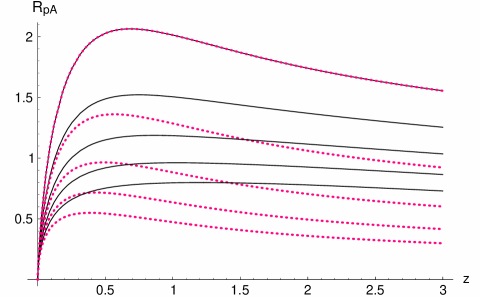
Figure 8: The Cronin ratio $\mathcal{R}_{pA}(z)$ (with $z\equiv k_{\perp}^{2}/Q_{s}^{2}(A)$) below and near the saturation scale for $\rho_{A}=6$. The solid lines correspond to an evolved nuclear wavefunction by $\Delta Y\ll 1$. The dotted lines correspond to an unevolved one (MV). The proton wavefunction is always given by the DLA solution. The curves, from top to bottom, correspond to $\Delta Y=n/(2\rho_{A})$ with $n=0,1,...,4$.

References

- (1) L. McLerran, R. Venugopalan, Phys. Rev. D49 (1994) 2233; ibid. 3352; ibid. 50 (1994) 2225.
- (2) E. Iancu, A. Leonidov and L. McLerran, Nucl. Phys. A692 (2001) 583; Phys. Lett. B510 (2001) 133; E. Ferreiro, E. Iancu, A. Leonidov and L. McLerran, Nucl. Phys. A703 (2002) 489.
-
(3)
E. Iancu, A. Leonidov and L. McLerran, The Colour Glass
Condensate: An Introduction, hep-ph/0202270.
Published in QCD Perspectives on Hot and Dense Matter, Eds. J.-P. Blaizot and E. Iancu,
NATO Science Series, Kluwer, 2002;
E. Iancu, R. Venugopalan, The Color Glass Condensate and High Energy Scattering in QCD, hep-ph/0303204. In Quark-Gluon Plasma 3, Eds. R. C. Hwa and X.-N. Wang, World Scientific, 2003. - (4) L.V. Gribov, E.M. Levin, and M.G. Ryskin, Phys. Rept. 100 (1983) 1; A.H. Mueller and J. Qiu, Nucl. Phys. B268 (1986) 427; J.-P. Blaizot and A. H. Mueller, Nucl. Phys. B289 (1987) 847.
- (5) M. Gyulassy, L. McLerran, New Forms of QCD Matter Discovered at RHIC, nucl-th/0405013.
- (6) “Quark Matter 2002”, Proceedings of the 16th International Conference on Ultra-Relativistic Nucleus-Nucleus Collisions, (Nantes, France 18-24 July, 2002), Nucl. Phys. A 715 (2003).
- (7) “Quark Matter 2004”, Proceedings of the 17th International Conference on Ultra-Relativistic Nucleus-Nucleus Collisions, (Oakland, USA, 11-17 January 2004), J. Phys. G30 (2004) S633-S1429.
- (8) A. Krasnitz, Y. Nara and R. Venugopalan, Phys. Rev. Lett. 87 (2001) 192302; Nucl. Phys. A 727 (2003) 427.
- (9) D. Kharzeev, M. Nardi, Phys. Lett. B507 (2001) 121; D. E. Kharzeev, E. Levin, Phys. Lett. B523 (2001) 79.
- (10) Yu.V. Kovchegov, Phys. Rev. D54 (1996) 5463; Phys. Rev. D55 (1997) 5445.
- (11) J. Jalilian-Marian, A. Kovner, L. McLerran, H. Weigert, Phys. Rev. D55 (1997) 5414.
- (12) Yu.V. Kovchegov and A.H. Mueller, Nucl. Phys. B529 (1998) 451.
- (13) E. Iancu, K. Itakura, and L. McLerran, Nucl. Phys. A708 (2002) 327; Nucl. Phys. A724 (2003) 181.
- (14) A. H. Mueller and D.N. Triantafyllopoulos, Nucl. Phys. B640 (2002) 331.
- (15) D.N. Triantafyllopoulos, Nucl. Phys. B648 (2003) 293.
- (16) A. H. Mueller, Nucl. Phys. A724 (2003) 223.
- (17) F. Gelis and J. Jalilian-Marian, Phys. Rev. D67 (2003) 074019.
- (18) J. Jalilian-Marian, Y. Nara and R. Venugopalan, Phys. Lett. B577 (2003) 54.
- (19) D. E. Kharzeev, E. Levin, and L. McLerran, Phys. Lett. B561 (2003) 93.
- (20) D. Kharzeev, Yu. V. Kovchegov, and K. Tuchin, Phys. Rev. D66 (2003) 094013; hep-ph/0405045.
- (21) R. Baier, A. Kovner and U. A. Wiedemann, Phys. Rev. D 68 (2003) 054009.
- (22) J. L. Albacete, N. Armesto, A. Kovner, C. A. Salgado and U. A. Wiedemann, Phys. Rev. Lett. 92 (2004) 082001.
- (23) See for example, D. d’Enterria, Hard scattering at RHIC: Experimental review, nucl-ex/0309015 and references therein.
- (24) S. Munier and R. Peschanski, Phys. Rev. Lett. 91 (2003) 232001; Phys. Rev. D69 (2004) 034008; hep-ph/0401215.
- (25) A.M. Staśto, K. Golec-Biernat, and J. Kwieciński, Phys. Rev. Lett. 86 (2001) 596.
- (26) For a review, see M. Gyulassy, I. Vitev, X. N. Wang and B. W. Zhang, Jet quenching and radiative energy loss in dense nuclear matter, arXiv:nucl-th/0302077. Published in Quark Gluon Plasma 3, editors: R.C. Hwa and X.N. Wang, World Scientific, Singapore, 2003.
- (27) B. B. Back et al. [PHOBOS Collaboration], Phys. Rev. Lett. 91 (2003) 072302 [arXiv:nucl-ex/0306025]; S. S. Adler et al. [PHENIX Collaboration], Phys. Rev. Lett. 91 (2003) 072303 [arXiv:nucl-ex/0306021]; J. Adams et al. [STAR Collaboration], Phys. Rev. Lett. 91 (2003) 072304 [arXiv:nucl-ex/0306024]; I. Arsene et al. [BRAHMS Collaboration], Phys. Rev. Lett. 91 (2003) 072305 [arXiv:nucl-ex/0307003].
- (28) I. Arsene [BRAHMS Collaboration], On the evolution of the nuclear modification factors with rapidity and centrality in d+Au collisions at = 200 GeV, nucl-ex/0403005.
- (29) I. Balitsky, Nucl. Phys. B463 (1996) 99; Phys. Rev. Lett. 81 (1998) 2024; Phys. Lett. B518 (2001) 235; High-energy QCD and Wilson lines, hep-ph/0101042.
- (30) Yu. V. Kovchegov, Phys. Rev. D60 (1999), 034008; ibid. D61 (2000) 074018.
- (31) E. Iancu, K. Itakura, and D.N. Triantafyllopoulos, Nucl. Phys. A742 (2004) 182.
- (32) J.R. Forshaw and D.A. Ross, Quantum Chromodynamics and the Pomeron, Cambridge University Press, Cambridge, 1997.
- (33) A. Dumitru and L. McLerran, Nucl. Phys. A700 (2002) 492.
- (34) Yu. V. Kovchegov and K. Tuchin, Phys. Rev. D65 (2002) 074026.
- (35) J.P. Blaizot, F. Gelis, R. Venugopalan, hep-ph/0402256; hep-ph/0402257, Nucl. Phys. A, to appear.
- (36) M. Braun, Eur. Phys. J. C16 (2000) 337; Phys. Lett. B483 (2000) 105.
- (37) L.N. Lipatov, Sov. J. Nucl. Phys. 23 (1976) 338; E.A. Kuraev, L.N. Lipatov and V.S. Fadin, Zh. Eksp. Teor. Fiz 72, 3 (1977) (Sov. Phys. JETP 45 (1977) 199); Ya.Ya. Balitsky and L.N. Lipatov, Sov. J. Nucl. Phys. 28 (1978) 822.
- (38) J. Jalilian-Marian, A. Kovner, A. Leonidov and H. Weigert, Nucl. Phys. B504 (1997) 415; Phys. Rev. D59 (1999) 014014.
- (39) H. Weigert, Nucl. Phys. A703 (2002) 823.
- (40) E. Iancu and L. McLerran, Phys. Lett. B510 (2001) 145.
- (41) A. H. Mueller, Phys. Lett. B523 (2001) 243.
- (42) E. Iancu, K. Itakura and S. Munier, Phys. Lett. B590 (2004) 199.
- (43) D. Boer and A. Dumitru, Phys. Lett. B556 (2003) 33 [arXiv:hep-ph/0212260].