We consider the Yukawa couplings for quarks and leptons in the context of Pati-Salam model using intersecting D-brane models where the Yukawa coupling matrices are rank one in a simple choice of family replication. The CKM mixings can be explained by perturbing the rank 1 matrix using higher order terms involving new Higgs fields available in the model. We show that the near bi-large neutrino mixing angles can be naturally explained, choosing the light neutrino mass matrix to be type II seesaw dominant. The predicted value of $U_{e3}$ is in the range $\simeq 0.05-0.15$. In the quark sector, $V_{cb}$ is naturally close to the strange/bottom quark mass ratio and we obtain an approximate relation $V_{ub}V_{cb}\simeq({m_{s}}/{m_{b}})^{2}V_{us}\,$. The geometrical interpretations of the neutrino mixings are also discussed.

1 Introduction

Understanding the masses and the mixings of quarks and leptons is one of the most important issues in particle physics. In the quark sector, there are 6 quark masses, $(m_{u},m_{c},m_{t})$ for up-type quarks and $(m_{d},m_{s},m_{b})$ for down-type quarks. For the quark mixing, there are 3 mixing angles in the CKM (Cabibbo-Kobayashi-Maskawa) matrix, and 1 phase. The masses are hierarchical and none of the mixing angles is large. Although those 10 parameters are completely free in the standard model, there may exist certain relations among the mass ratios and the mixing angles [1].

On the other hand, in the leptonic sector, there are 3 charged-lepton masses $(m_{e},m_{\mu},m_{\tau})$, whose hierarchical pattern is similar to the down-type quark ones, though it is not completely same [2]. Recent neutrino experiments show that neutrinos also have masses and it was revealed [3, 4] that the two neutrino mixing angles to explain the atmospheric and solar neutrino data are large (especially, the best fit for atmospheric mixing is maximal), while another mixing angle $\theta_{13}$ is small as required to satisfy the long baseline neutrino data [5]. In fact, these hierarchical mass patterns and this combination of small and large mixing angles may be a key issue to select models beyond the standard model and to explain the origin of flavors. In the framework of the standard model, there is no relation between the quark sector and the leptonic sector. It is discussed whether the quark and lepton masses and mixings can be related in an unification pictures [6].

Even if the unified gauge models are considered, the Yukawa couplings are fundamental parameters in four-dimensional field theory. In that case, the existence of more fundamental theories are expected to describe the variety of quark and lepton masses and mixings. String theory is a most promising candidate to describe particle field theories as an effective theory, as well as quantum gravity. String theory is attractive because all the parameters can be calculated from a few fundamental parameters. But there has been no clear answer on how to derive the standard model in string theory since the selection of vacua may be a non-perturbative phenomena. However, the non-perturbative aspects of string theories can be discussed, once the D-branes were formulated [7]. Indeed, the intersecting D-branes [8, 9] are interesting approaches to construct the standard model. The $N$ stack of D-branes can form $U(N)$ gauge fields, and at the intersection between the $N$ stack and $M$ stack of D-branes, a massless chiral fermion belonging to $(N,\bar{M})$ bi-fundamental representation can appear. Such a situation is very attractive to obtain quark and lepton fields not only in the standard model but also in the models where the gauge group is given as direct group such as Pati-Salam model [10]. In addition to the realization of the particle representation and the gauge groups of the standard-like models, the Yukawa couplings are calculable in the intersecting D-brane models [11, 12, 13]. The couplings are described as $e^{-kA}$ naively by the triangle area $A$ formed by the three intersecting points. The presence of the exponential factors can be utilized to achieve the hierarchical pattern of fermion masses.

Since the intersecting D-brane models have potentials to explain the pattern of fermion masses and mixings, many people have constructed various intersecting D-brane models [14, 15, 16, 17]. One interesting issue is that in the simple models, Yukawa matrices are written as factorized form $y_{ij}=x^{L}_{i}x^{R}_{j}$ [11, 18]. This originates from a geometrical reason that the left- and right-handed fermions are replicated at the intersecting points on the different tori, and the Yukawa couplings are given as an exponential form of sum of the triangle areas. As a result of the factorized form of Yukawa coupling, the Yukawa matrices are rank 1, and thus only the 3rd generation fermions are massive. In order to construct a realistic model, this issue for Yukawa matrices needs to be resolved and several possibilities have been considered in the literature [18, 19, 20].

In this paper, we emphasize the possibility that the rank 1 Yukawa matrices are crucial to understand the properties of fermion mixings. The Pati-Salam model can be constructed using intersecting D-branes with several attractive features [16]. This model has left-right gauge symmetry $SU(2)_{L}\times SU(2)_{R}$ and an up-down symmetry is exhibited if there is only one Higgs bidoublets. This up-down symmetry must be broken since the up- and the down-type quark masses have different hierarchical pattern and the CKM matrix is not an identity matrix. Consequently, new Higgs fields must be introduced to break up-down symmetry. The extra Higgs fields are also needed to raise the rank of the Yukawa matrices. In fact, there are extra Higgs fields at the intersection between visible branes and hidden branes, which is needed to satisfy the RR tadpole cancellation condition. Such extra Higgs fields can contribute to produce the Yukawa matrices through higher order terms, and hierarchies of the fermion masses can be realized. We also study the consequences that the Yukawa couplings are given as rank 1 matrices plus small corrections. We will show that the observed small mixings in quark sector can be easily realized, and in the lepton sector, the solar and the atmospheric mixings for neutrino oscillation, are generically large while one other mixing is small. We will also study the geometrical interpretation of the neutrino mixings.

This paper is organized as follows: In section 2, we construct intersecting D-brane models with the Pati-Salam gauge symmetry. In section 3, the Yukawa matrices in the intersecting D-brane models are studied and we discuss how the almost rank 1 Yukawa matrices are realized. In section 4, we show the consequences of the fact that Yukawa matrices are almost rank 1 matrix. In section 5, we will see that the observed properties of neutrino mixings can be interpreted in geometrical way. The section 6 is devoted to conclusions and discussions.

2 Pati-Salam like model from intersecting D-branes

In this section, we will briefly discuss the construction of a model, in the type IIA orientifolds on $T^{6}/Z_{2}\times Z_{2}$ with intersecting D6-branes [21]. The supersymmetric Pati-Salam models with gauge symmetry $U(4)_{c}\times U(2)_{L}\times U(2)_{R}\times G_{h}$ are constructed in the Ref. [16]. There are D6_a-brane for $U(4)_{c}$, D6_b-brane for $U(2)_{L}$, D6_c-brane for $U(2)_{R}$. Extra branes are needed to cancel RR tadpole. We call such extra branes D6_1,2-branes which provide hidden $USp$ gauge groups.

At the intersection between the D6_a-brane and the D6_b-brane, for example, open strings can stretch and chiral fermions belonging to bi-fundamental representation $(\bf{4,{\bar{2}},1})$ can appear as a zero mode which corresponds to the left-handed matter fields. The right-handed matter fields $(\bf{{\bar{4}},1,2})$ can be located at the intersection between the D6_a-brane and the D6_c-brane. The Higgs bidoublet $({\bf 1,2,{\bar{2}}})$ is at the intersection between the D6_b-brane and the D6_c-brane. The family is replicated when the six dimensions are compactified to the torus $T^{6}=T^{2}\times T^{2}\times T^{2}$. The family number is given by the intersecting number

$$I_{\alpha\beta}=\prod_{i=1}^{3}(n_{\alpha}^{i}m_{\beta}^{i}-m_{\alpha}^{i}n_{\beta}^{i}),$$ (1)

using wrapping numbers $(n_{\alpha}^{i},m_{\alpha}^{i})$ for each torus $(i=1,2,3)$, which specifies that the D6_α-branes are stretching over our three-dimensional space. An orientifold, which is needed to have negative contribution to the vacuum energy, can be constructed by discrete transformation with world sheet parity. The orientifold image of $\alpha$ brane is denoted as $\alpha^{\prime}$. The wrapping numbers of the $\alpha^{\prime}$ are given as $(n_{\alpha}^{i},-m_{\alpha}^{i})$. In order to obtain odd numbers of chiral families in this model, we need one tilted torus, and for the tilted torus we have $\tilde{m}_{\alpha}^{i}=m_{\alpha}^{i}+\frac{1}{2}n_{\alpha}^{i}$ and the wrapping number of the orientifold image is $(n_{\alpha}^{i},-\tilde{m}_{\alpha}^{i})$. The wrapping numbers are constrained by the RR tadpole cancellation and the supersymmetry preserving conditions. The wrapping numbers for the supersymmetric Pati-Salam models with three chiral families are systematically searched in Ref.[16]. An example of wrapping numbers from one of the models in Ref.[16] is given in Table 1.

	$N_{\alpha}$	$(n^{1}_{\alpha},m^{1}_{\alpha})$	$(n^{2}_{\alpha},m^{2}_{\alpha})$	$(n^{3}_{\alpha},\tilde{m}^{3}_{\alpha})$
$a$	$8$	$(0,-1)$	$(1,1)$	$(1,1/2)$
$b$	$4$	$(3,1)$	$(1,0)$	$(1,-1/2)$
$c$	$4$	$(1,0)$	$(1,4)$	$(1,-1/2)$
$1$	$4$	$(0,-1)$	$(0,1)$	$(2,0)$
$2$	$2$	$(0,-1)$	$(1,0)$	$(0,1)$

Table 1: An example of wrapping numbers to obtain supersymmetric Pati-Salam model with three chiral families.

The number $N_{\alpha}$ in Table 1 denotes the stack number of the $\alpha$ brane. In the $T^{6}/Z_{2}\times Z_{2}$ orbifold model, $N_{\alpha}$ stack of branes generates gauge symmetry $U(N_{\alpha}/2)$. For the branes which parallel to the orientifolds, $USp(N_{\alpha})$ gauge symmetry is generated. So the gauge symmetry for the wrapping numbers shown in Table 1 is $U(4)_{c}\times U(2)_{L}\times U(2)_{R}\times USp(4)_{1}\times USp(2)_{2}$.

sector	rep.	$Q_{4}$	$Q_{2L}$	$Q_{2R}$	$Q^{\prime}$	field
$ab$	$(\bf{4,\bar{2},1})$	1	$-1$	0	0	$\psi$
$ac$	$({\bar{\bf{4}},\bf 1,2})$	$-1$	0	1	0	$\psi^{c}$
$bc$	$(\bf{1,2,{\bar{2}}})$	0	1	$-1$	0	$H$
$a1$	$(\bf{4,1,1})$	1	0	$0$	$\pm 1$	$X$
$b1$	$(\bf{1,{2},1})$	0	$1$	$0$	$\pm 1$	$h$
$c1$	$(\bf{1,1,{\bar{2}}})$	0	0	$-1$	$\pm 1$	$h^{c}$

Table 2: The relevant fields to construct a semi-realistic model. The conjugate representations are denoted as $\bar{X}$, for example.

We list relevant fields to construct our model in Table 2. The $Q_{4}$, $Q_{2L}$, and $Q_{2R}$ are the charges for $U(1)$’s which are subgroups of $U(4)_{c}$, $U(2)_{2L}$, $U(2)_{2R}$. Those three $U(1)$ symmetries are anomalous and their gauge bosons become massive by generalized Green-Schwarz mechanism [22]. The $Q^{\prime}$ denotes the $U(1)$ charge embedded in $USp(4)$. The $USp(4)$ symmetry is broken to $U(1)$ by splitting away the branes from the orientifolds on all three tori, which is equivalent to Higgsing of $USp(4)$ by three antisymmetric chiral multiplets which are massless modes [23]. The fundamental representation of $USp(4)$ group has $\pm 1$ charges under the $U(1)$ subgroup. The hypercharge of the fields can be defined as

$$Y=T_{2R}^{3}+\frac{B-L}{2}+\frac{Q^{\prime}}{2}\,.$$ (2)

The $B-L$ is a $U(1)$ generator, diag.($1/3,1/3,1/3,-1$), in the $SU(4)_{c}\rightarrow SU(3)_{c}\times U(1)_{B-L}$. The $SU(4)_{c}\times SU(2)_{R}$ symmetry can be broken to $SU(3)_{c}\times U(1)_{B-L}\times U(1)_{R}$ by the brane splitting. The vacuum expectation value of $h^{c}$ breaks $U(1)_{R}\times U(1)_{USp}$ symmetry to $U(1)_{R}^{\prime}$. The brane splitting is equivalent to the Higgsing by adjoint fields for $SU(4)_{c}$ and $SU(2)_{R}$ in the effective field theory, thus Yukawa couplings for top, bottom and tau may be almost unified since the breaking terms are higher order.

We note that the model is consistent when we consider the confining phase of $USp(4)$ where $hh^{c}$ is confined to be the bidoublet Higgs fields. Also, $Xh$ (and $X\bar{h}$) can be confined to form the matter representation, and hence, $X$ should be vector-like to maintain chiral three generations. When the confining field $\bar{X}h^{c}$ acquires vacuum expectation values, $SU(4)_{c}\times SU(2)_{R}$ is broken down to $SU(3)_{c}\times U(1)_{Y}$. The beta functions for the $USp$ groups are negative for the model shown in the Table 2. The confining $USp$ gauge groups may be interesting since it may break the supersymmetry by gaugino condensation mechanism [24].

Furthermore, both left- and right-handed neutrino Majorana mass terms can be generated by the non-renormalizable interaction in the superpotential,

$$\frac{1}{M_{s}^{3}}f_{ij}\psi_{i}\psi_{j}\,[\bar{X}h\bar{X}h]+\frac{1}{M_{s}^{3}}f_{ij}^{c}\psi^{c}_{i}\psi^{c}_{j}\,[Xh^{c}Xh^{c}]\,.$$ (3)

The $USp$ confinement can produce $SU(2)_{L,R}$ triplets with proper hypercharges, $[\bar{X}h\bar{X}h]\sim\Lambda^{3}\bar{\Delta}_{L}$ and $[Xh^{c}Xh^{c}]\sim\Lambda^{3}\Delta_{R}$, where $\Lambda$ is a confining scale of $USp$ group. Once $SU(2)_{L}$ triplet acquires a small vacuum expectation value around sub-eV range and $SU(2)_{R}$ triplet acquires a vacuum expectation value around the confining scale, the seesaw neutrino masses [25],

$$m_{\nu}^{\rm light}=M_{L}-M_{\nu}^{D}M_{R}^{-1}(M_{\nu}^{D})^{T},$$ (4)

are generated, where $M_{\nu}^{D}$ is a neutrino Dirac mass matrix and $M_{L}$ and $M_{R}$ are left- and right-handed neutrino Majorana mass matrices which are proportional to $f$ and $f^{c}$.

3 Yukawa couplings

The Yukawa couplings,

$$W=y_{ij}\psi_{i}\psi^{c}_{j}H,$$ (5)

are generated from world sheet instanton corrections and is written by using Jacobi theta function in the form [11],

$$y_{ij}\propto\prod_{r=1}^{3}\vartheta\left[\begin{array}[]{c}\delta^{(r)}\\ \phi^{(r)}\end{array}\right](\kappa^{(r)})\,,\quad\vartheta\left[\begin{array}[]{c}\delta\\ \phi\end{array}\right](\kappa)=\sum_{\ell\in{\bf Z}}e^{-\pi\kappa(\delta+\ell)^{2}}e^{2\pi i(\delta+\ell)\phi},$$ (6)

where $\delta^{(r)}$ characterizes intersections and shifts of the D-branes in each torus, $\kappa^{(r)}$ represents a Kähler structure, and $\phi$ is for a possible Wilson-line phase.

It is important that the Yukawa couplings are given in a factorized form. As a result, when the family of left- and right-handed matters are replicated in different tori as in the example given in Table 1, the Yukawa matrices of quarks and leptons are given as $y_{ij}\propto x_{i}^{L}x_{j}^{R}$. Then, the Yukawa matrix $y_{ij}$ is rank 1, and thus, only the third generation fermions can acquire masses by Higgs mechanism. When the family is replicated in the same torus, the Yukawa matrix turns out to be diagonal and no mixing arises when there is only one Higgs field. Several discussions exist describing this property [18, 19, 20].

The rank 1 property is an interesting feature of the intersecting D-brane models as we will see in the subsequent sections. In this section, we will suggest a possibility of raising the rank.

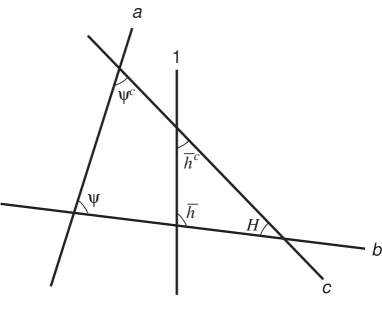
Figure 1: A sketch of intersections.

Let us suppose that the $USp$ brane passes across the triangle formed by the $abc$ branes as shown in Figure 1. Then the Higgs coupling $H\bar{h}\bar{h}^{c}$ arises in the superpotential along with the Yukawa coupling $y\,\psi\psi^{c}H$. As was calculated in [12], from the quadrangle $ab1c$, a four-fermi interaction $y^{\prime}\psi\psi^{c}\tilde{\bar{h}}\tilde{\bar{h^{c}}}/M_{s}^{2}$ can arise which corresponds to a higher order term in the Kähler potential. In non-supersymmetric models, the four-fermi interaction can produce a Yukawa coupling by a loop diagram [19]. In supersymmetric models, such a loop effect is cancelled by a bosonic loop through the interaction $y^{\prime}\psi\psi^{c}F_{\bar{h}}^{*}\bar{h}^{c}{}^{\dagger}$, where $F_{\bar{h}}^{*}\sim H\bar{h}^{c}$. However, in our model construction, $\bar{h}^{c}$ can acquire a vacuum expectation value, and thus a new Yukawa coupling, $\displaystyle y^{\prime}\frac{\langle\bar{h}^{c}\rangle^{2}}{M_{s}^{2}}\psi\psi^{c}H$, can be produced from a Kähler potential term directly. Contrary to a three-point function, the coupling $y^{\prime}$ does not factorize in general since it involves a four-point function [12, 19]. This is due to the fact that there are more parameters in the four point function and only in certain limiting cases one obtains the factorizable result. Therefore, due to the existence of the $USp$ branes, which may be needed to cancel the RR tadpole, the fermions of 1st and 2nd generations can acquire masses both in supersymmetric and non-supersymmetric scenarios. When the massless chiral Higgs fields are $h$ and $h^{c}$ instead of $\bar{h}$ and $\bar{h}^{c}$, the superpotential term $\psi\psi^{c}hh^{c}$ will be produced and will contribute to fermion masses. We note that the structure is consistent when we consider the confining phase of $USp$ gauge group. In that case, the second generation masses are suppressed by the ratio of the confining scale and the string scale. When the beta function of $USp$ group is negative, the mass hierarchy can be naturally explained.

We note that the Higgs bidoublet may acquire a large mass through the $H\bar{h}\bar{h}^{c}$ coupling when $\bar{h}^{c}$ gets a vacuum expectation value around the string scale. However, since there exists $SU(2)_{L}$ singlets in the $bb^{\prime}$ sector, one can obtain bilinear masses of $H$ and $\bar{h}$ and thus a linear combination can be made to be light. In any case, such mixings may be needed to break the up-down quark mass symmetry arising from the existence of an $SU(2)_{R}$ symmetry.

4 Properties of “almost rank 1” Yukawa matrix

In the previous section, we discussed the construction of the Pati-Salam model. In the model, the Yukawa coupling can be a rank 1 matrix plus small contributions from higher order terms. We will call such a Yukawa matrix as “almost rank 1 matrix”. One may think that there is no prediction once the higher order terms are added. However, such an almost rank 1 matrix gives us several qualitative features for the fermion masses and mixings. For example, the masses of 1st and 2nd generations can be hierarchically smaller than the masses of the 3rd generation. For the mixings, there are interesting qualitative properties as well. In this section, we will see the properties of fermion mixings in a general framework which does not depend very much on the details of the model.

The Yukawa matrices for quarks and leptons are approximately given as rank 1 matrices $y_{ij}=x_{i}^{L}x_{j}^{R}$. For simplicity, let us consider the symmetric matrix $x^{L}=x^{R}$. It can be easily extended to the case of non-symmetric matrices. The rank 1 matrix is written as

$$Y_{0}=\left(\begin{array}[]{c}c\\ b\\ a\end{array}\right)\left(\begin{array}[]{ccc}c&b&a\end{array}\right)=\left(\begin{array}[]{ccc}c^{2}&bc&ac\\ bc&b^{2}&ab\\ ac&ab&a^{2}\end{array}\right).$$ (7)

The parameters $a,b,c$ can be made real, and are generically $O(1)$ parameters. We obtain a useful unitary matrix to diagonalize the rank 1 matrix :

$$U_{0}Y_{0}U_{0}^{T}={\rm diag}(0,\ 0,\ a^{2}+b^{2}+c^{2}),$$ (8)

$$U_{0}=\left(\begin{array}[]{ccc}\frac{b}{\sqrt{b^{2}+c^{2}}}&-\frac{c}{\sqrt{b^{2}+c^{2}}}&0\\ \frac{ac}{\sqrt{b^{2}+c^{2}}\sqrt{a^{2}+b^{2}+c^{2}}}&\frac{ab}{\sqrt{b^{2}+c^{2}}\sqrt{a^{2}+b^{2}+c^{2}}}&-\frac{\sqrt{b^{2}+c^{2}}}{\sqrt{a^{2}+b^{2}+c^{2}}}\\ \frac{c}{\sqrt{a^{2}+b^{2}+c^{2}}}&\frac{b}{\sqrt{a^{2}+b^{2}+c^{2}}}&\frac{a}{\sqrt{a^{2}+b^{2}+c^{2}}}\end{array}\right).$$ (9)

It is useful to parameterize as

$$a=\sqrt{y}\cos\theta_{a},\quad b=\sqrt{y}\sin\theta_{a}\cos\theta_{s},\quad c=\sqrt{y}\sin\theta_{a}\sin\theta_{s}\,.$$ (10)

It is important to note here that there are only two independent angles in the unitary matrix. Since two of the eigenvalues are zero, the corresponding eigenvectors can be rotated to a linear combinations of the 1st and 2nd row vectors in the unitary matrix. However, when the rank 1 matrix is perturbed to raise the rank, it can be easily checked that this basis is useful to perturb in the limit where the 1st generation is massless.

Let us consider “almost rank 1” Yukawa matrices for quarks as

$$Y_{u}=Y_{0}+\tilde{Y}_{u},\qquad Y_{d}=Y_{0}+\tilde{Y}_{d}\,.$$ (11)

The $\tilde{Y}_{u,d}$ are perturbation matrices. Let us start on a basis where $\tilde{Y}_{d}$ is diagonal,

$$\tilde{Y}_{d}={\rm diag}(\epsilon_{1},\epsilon_{2},\epsilon_{3}).$$ (12)

To obtain the hierarchical quark masses, we need to assume $\epsilon_{1},\epsilon_{2}\ll\epsilon_{3}\ll a,b,c$. The eigenvalues of the down-type Yukawa matrix are approximately

$$y_{b}\simeq y,\quad y_{s}\simeq\sin^{2}\theta_{a}^{q}\epsilon_{3},\quad y_{d}\simeq\cos^{2}\theta_{s}^{q}\epsilon_{1}+\sin^{2}\theta_{s}^{q}\epsilon_{2}+\cot^{2}\theta_{a}^{q}\epsilon_{1}\epsilon_{2}/\epsilon_{3}.$$ (13)

To make the basis clear, we have attached the superscript $q$ to $\theta_{a}$ and $\theta_{s}$. In this basis, $\tilde{Y}_{u}$ is not necessarily diagonal, but it is reasonable to assume that $\tilde{Y}_{u}$ is almost aligned to $\tilde{Y}_{d}$.

Defining the unitary matrix $V_{u},V_{d}$ such that $V_{u}Y_{u}V_{u}^{T}$ and $V_{d}Y_{d}V_{d}^{T}$ are diagonal, we obtain the CKM matrix as $V_{\rm CKM}=V_{u}V_{d}^{\dagger}$. Although $V_{u}$ and $V_{d}$ include large mixing angles in $U_{0}$, such large mixings are canceled out in the CKM matrix because the left-handed rotation $U_{0}$ is common in $Y_{u}$ and $Y_{d}$. We note that even if we do not have the left-right symmetry, the left-handed rotation is common in the formulation of the model, $Y_{0}^{(u,d)}{}_{ij}=x^{L}_{i}x_{j}^{R(u,d)}$. One can define unitary matrices $\tilde{V}_{u,d}$ such that $V_{u,d}=\tilde{V}_{u,d}U_{0}$ and $V_{\rm CKM}=\tilde{V}_{u}\tilde{V}_{d}^{\dagger}$. The $\tilde{V}_{d}$ is the diagonalizing matrix of $U_{0}Y_{d}U_{0}^{T}$:

$$U_{0}Y_{d}U_{0}^{T}\simeq\left(\begin{array}[]{ccc}\cos^{2}\theta_{s}^{q}\epsilon_{1}+\sin^{2}\theta_{s}^{q}\epsilon_{2}&\frac{1}{2}(\epsilon_{1}-\epsilon_{2})\cos\theta_{a}^{q}\sin 2\theta_{s}^{q}&\frac{1}{2}(\epsilon_{1}-\epsilon_{2})\sin\theta_{a}^{q}\sin 2\theta_{s}^{q}\\ \frac{1}{2}(\epsilon_{1}-\epsilon_{2})\cos\theta_{a}^{q}\sin 2\theta_{s}^{q}&\sin^{2}\theta_{a}^{q}\epsilon_{3}&-\frac{1}{2}\sin 2\theta_{a}^{q}\epsilon_{3}\\ \frac{1}{2}(\epsilon_{1}-\epsilon_{2})\sin\theta_{a}^{q}\sin 2\theta_{s}^{q}&-\frac{1}{2}\sin 2\theta_{a}^{q}\epsilon_{3}&y+\cos^{2}\theta_{a}^{q}\epsilon_{3}\end{array}\right).$$ (14)

Since the up-type quarks are more hierarchical than the down-type ones, one can expect that $V_{\rm CKM}\simeq\tilde{V}_{d}^{\dagger}$. We then obtain $V_{cb}\simeq\frac{1}{2}\sin 2\theta_{a}^{q}\epsilon_{3}/y$, or,

$$V_{cb}\simeq\cot\theta_{a}^{q}\ \frac{m_{s}}{m_{b}}\,.$$ (15)

Since $a,b,c$ are expected to be $O(0.1)$ parameters, we obtain $V_{cb}\sim m_{s}/m_{b}$ as a string scale relation which is in agreement with experiments [26]. We have little more flexibility to fit the other two angles. Now we set the famous empirical relation $V_{us}\simeq\sqrt{m_{d}/m_{s}}$ as input. In order to do so we assume $(U_{0}Y_{d}U_{0}^{T})_{11}\simeq 0$, which leads to $\epsilon_{1}\simeq-\tan^{2}\theta_{s}^{q}\epsilon_{2}$. Using this relation we obtain $V_{us}\simeq\cos\theta_{a}^{q}/\sin^{2}\theta_{a}^{q}\tan\theta_{s}^{q}\epsilon_{2}/\epsilon_{3}$, $V_{ub}\simeq\sin\theta_{a}^{q}\tan\theta_{s}^{q}\epsilon_{2}/y$. We finally obtain the following relation

$$V_{ub}V_{cb}\simeq\left(\frac{m_{s}}{m_{b}}\right)^{2}V_{us}\,,$$ (16)

which is again in good agreement with experiments. The Kobayashi-Maskawa phase can be derived from a phase of $\epsilon_{3}$.

Next, let us go on to the leptonic sector. If type I seesaw contribution (i.e. $M_{\nu}^{D}M_{R}^{-1}(M_{\nu}^{D})^{T}$) is dominant, the large mixings in $Y_{0}$ are canceled between the charged-lepton and the neutrino Dirac Yukawa couplings, in the same way as it happens in the CKM matrix. However, if the type I contributions are suppressed due to a large right-handed Majorana mass scale, the large mixings can directly appear in general. We therefore consider the case where $M_{L}$ dominates in the light neutrino mass formula, Eq.(4). We start in the basis where the light neutrino mass matrix is diagonal. The charged-lepton Yukawa matrix is given as

$$Y_{e}=Y_{0}^{l}+\tilde{Y}_{e}.$$ (17)

We note that $Y_{0}^{l}$, given in the above basis, may be different from the $Y_{0}$ where $\tilde{Y}_{d}$ is diagonal even if the $SU(4)_{c}$ unification is exact. However, $a^{l},b^{l},c^{l}$ in $Y_{0}^{l}$ are all $O(1)$ parameters in general in this basis. (We have attached the superscript $l$ to avoid any confusion). The $\tilde{Y}_{e}$ is not necessarily diagonal in this basis, but it may be reasonable that the $\tilde{Y}_{e}$ is close to diagonal since it is hierarchical.

The Maki-Nakagawa-Sakata-Pontecorvo (MNSP) matrix for neutrino oscillation is given in the basis as $U_{\rm MNSP}=V_{e}^{*}$ where $V_{e}Y_{e}V_{e}^{T}$ is diagonal. The unitary matrix $\tilde{V}_{e}$ is defined as $V_{e}=\tilde{V}_{e}U_{0}^{l}$ and it is the diagonalization matrix of $U_{0}^{l}Y_{e}U_{0}^{l}{}^{T}$. The matrix $\tilde{V}_{e}$ can be parameterized as

$$\tilde{V}_{e}=\left(\begin{array}[]{ccc}c^{e}_{12}c^{e}_{13}&s^{e}_{12}c^{e}_{13}&s^{e}_{13}e^{i\delta}\\ -s^{e}_{12}c^{e}_{23}-c^{e}_{12}s^{e}_{23}s^{e}_{13}e^{-i\delta}&c^{e}_{12}c^{e}_{23}-s^{e}_{12}s^{e}_{13}s^{e}_{23}e^{-i\delta}&c^{e}_{13}s^{e}_{23}\\ s^{e}_{12}s^{e}_{23}-c^{e}_{12}c^{e}_{23}s^{e}_{13}e^{-i\delta}&-c^{e}_{12}s^{e}_{23}-s^{e}_{12}s^{e}_{13}c^{e}_{23}e^{-i\delta}&c^{e}_{13}c^{e}_{23}\end{array}\right)\left(\begin{array}[]{ccc}1&&\\ &e^{-i\alpha}&\\ &&e^{-i\beta}\end{array}\right).$$ (18)

Then 13 element of MNSP matrix, $U_{e3}$, can be calculated as

$$U_{e3}=\cos\theta_{a}^{l}e^{i(\beta-\delta)}s_{13}^{e}-\sin\theta_{a}^{l}e^{i\alpha}s_{12}^{e}c_{13}^{e}\,.$$ (19)

The charged-lepton masses are hierarchical, and thus we expect that all three mixing angles in $\tilde{V}_{e}$ are small in the same way as $\tilde{V}_{d}$. Since the up-type Yukawa is more hierarchical rather than the down-type one, we expect the relation $V_{\rm CKM}\simeq\tilde{V}_{d}^{\dagger}$ approximately. When we consider a quark-lepton unification, we can expect that $\tilde{V}_{e}\sim\tilde{V}_{d}\sim V_{CKM}^{\dagger}$. So, we neglect $s_{13}^{e}$, $s_{23}^{e}$, which are much smaller than $s_{12}^{e}$. Then we obtain three mixing angles, $\sin\theta_{13}\equiv|U_{e3}|$, $\tan\theta_{\rm sol}\equiv|U_{e2}/U_{e1}|$, and $\tan\theta_{\rm atm}\equiv|U_{\mu 3}/U_{\tau 3}|$, for the neutrino oscillation approximately,

$$\sin\theta_{13}\simeq\sin\theta_{a}^{l}s_{12}^{e}\,,$$ (20)

$$\tan\theta_{\rm atm}\simeq\tan\theta_{a}^{l}c_{12}^{e}\,,$$ (21)

$$\sin^{2}\theta_{\rm sol}\simeq\sin^{2}\theta_{s}^{l}\left(1-2\cot\theta_{s}^{l}\cos\theta_{a}^{l}t_{12}^{e}\cos\alpha+\frac{\cos 2\theta_{s}^{l}}{\sin^{2}\theta_{s}^{l}}\cos^{2}\theta_{a}^{l}t_{12}^{e2}\right),$$ (22)

where $t_{12}^{e}=s_{12}^{e}/c_{12}^{e}$. We note that an interesting approximate relation,

$$\theta_{\rm sol}\sim\theta_{s}^{l}\pm\theta_{13}\cot\theta_{\rm atm}\cos\alpha\,,$$ (23)

is satisfied. The Jarskog invariant of the MNSP matrix can be calculated as

$$J_{\rm MNSP}\simeq\frac{1}{8}\sin 2\theta_{12}^{e}\sin 2\theta_{a}^{l}\sin 2\theta_{s}^{l}\sin\theta_{a}^{l}\sin\alpha\,.$$ (24)

Neglecting a small $s_{12}^{e}(=\sin\theta_{12}^{e})$, we find that the phase $\alpha$ corresponds to the MNSP phase approximately up to a quadrant. Therefore, when CP violation in neutrino oscillation is maximal (which corresponds to $\sin\alpha=\pm 1$), the solar mixing angle is almost same as $\theta_{s}^{l}$.

Let us assume, for example, that $\theta_{a}$ and $\theta_{s}$ are maximal (45 degree), $\alpha=0$, $t_{12}^{e}>0$, and $s_{12}^{e}$ is the same as the Cabibbo angle ($s_{12}^{e}=0.22$). Then we find $\sin^{2}2\theta_{\rm atm}\simeq 1$, $\tan^{2}\theta_{\rm sol}\simeq 0.52$, $U_{e3}\simeq 0.15$ which are consistent with current experimental data.

The 12 mixing $s_{12}^{e}$ may be smaller than the Cabibbo angle by a factor 1/3 because the muon mass is a factor of 3 larger than the strange quark mass. So, $U_{e3}$ is expected to be in the range $0.05-0.15$.

Note that the bi-large mixing angles and a small $U_{e3}$ can be naturally obtained from the almost rank 1 charged-lepton Yukawa matrix. The two angles $\theta_{a}^{l}$ and $\theta_{s}^{l}$ are due to the rank 1 matrix and thus those are generically large mixings. On the other hand, $\theta_{13}$ is generated from perturbation matrix, and thus, it is naturally small. This qualitative feature does not depend on the details of the model.

5 Geometrical interpretation of neutrino mixings

In the previous section, we have seen that patterns of the observed quark and lepton mixings can be easily reproduced using the almost rank 1 Yukawa matrices. Although there are no rigid quantitative predictions, the qualitative feature is interesting especially for the neutrino mixings. The solar and atmospheric mixings are generically large and $\theta_{13}$ is small. The reason for $\theta_{13}$ mixing being small only can be explained geometrically i.e. the left- and the right-handed families are replicated on different tori. Further, we have seen that the solar and atmospheric mixings are almost same as the two angles in a rank 1 Yukawa matrix. So, these two mixings can be expressed by the Jacobi theta function as a function of moduli parameters, assuming that the mixings originating from left-handed Majorana mass matrix are small.

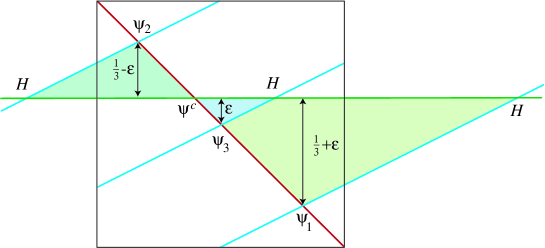
Figure 2: A sketch of brane intersections on a torus.

As we have supposed to obtain an almost rank 1 Yukawa matrix, $U(4)_{c}$ and $U(2)_{R}$ branes are intersecting once on the torus where the left-handed matter is replicated. So, let us assume that the intersecting numbers on a torus to be $|I_{ab}^{(r)}|=3$, $|I_{ac}^{(r)}|=1$ and $|I_{bc}^{(r)}|=1$ as shown in Figure 2. The ratio of the left-handed part $x^{L}_{i}=(c,b,a)$ of the rank 1 matrix, $y_{ij}=x^{L}_{i}x^{R}_{j}$, is written as

$$a:b:c=\vartheta\left[\begin{array}[]{c}\varepsilon\\ 0\end{array}\right](t):\vartheta\left[\begin{array}[]{c}-\frac{1}{3}+\varepsilon\\ 0\end{array}\right](t):\vartheta\left[\begin{array}[]{c}\frac{1}{3}+\varepsilon\\ 0\end{array}\right](t)\,.$$ (25)

The moduli parameter $\varepsilon$ represents a shift of the D-brane as shown in Figure 2, and $t=3A/\alpha^{\prime}$ where $A$ represents the Kähler structure of the torus. We neglect Wilson line phase for simplicity. When $t$ is large, which corresponds to a weak coupling limit, the ratio is determined by the area of each triangle forming by $\psi_{i}\psi^{c}H$. On the other hand, when $t$ is small, which corresponds to the strong coupling limit, the contributions from the triangles of larger sizes are not negligible. The shift parameter $\varepsilon$ corresponds to the vertical distance to the branes from the intersections where the left-handed matter fields replicate. The $\vartheta$ function is periodic for $\varepsilon$ which can be in the range $[0,1)$ in general. But we assume that $-\frac{1}{6}\leq\varepsilon\leq\frac{1}{6}$ to identify the closest intersection to be the third generation. Further, turning on the 1st and 2nd generations for $\varepsilon<0$, we get $0\leq\varepsilon\leq\frac{1}{6}$. In this range of $\varepsilon$, we obtain $a\geq b\geq c$. The angles $\theta_{s}$ and $\theta_{a}$ are calculated as functions of $\varepsilon$ and $t$, and they are plotted in the Figure 3 for different values of $\varepsilon$. As one can see in the figure that both mixings can be maximal.

Let us see the geometrical meaning of the behaviors of two mixings. At first, consider the case $\varepsilon=0$ which means that three branes are intersecting at one point in a torus. In this case, $b=c$ for any $t$, and then $\tan\theta_{s}=c/b=1$. When $\varepsilon\neq 0$, the triangle $\psi_{1}\psi^{c}H$ becomes larger than $\psi_{2}\psi^{c}H$ and thus $b>c$. Therefore, when $\varepsilon$ increases, $\theta_{s}$ is getting smaller. Another typical case for the shift parameter is $\varepsilon=\frac{1}{6}$. In this case, the triangle areas for $\psi_{3}$ and $\psi_{2}$ are same and thus $a=b$. Since $\tan\theta_{a}=\sqrt{b^{2}+c^{2}}/a$, the $\theta_{a}$ angle becomes maximal when $c$ (and therefore $\tan\theta_{s}$) gets exponentially damped for large $t$.

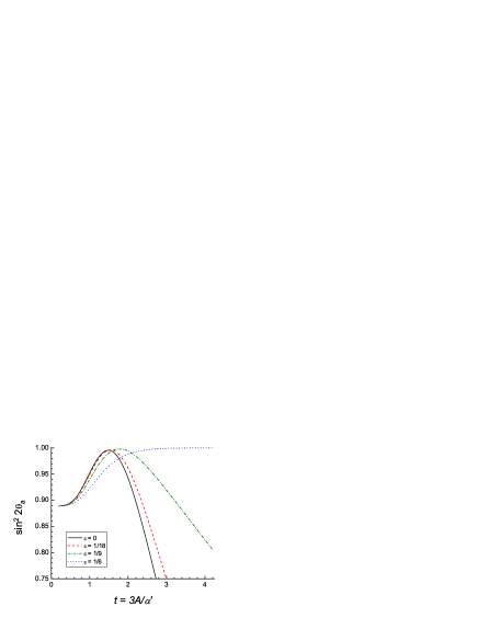
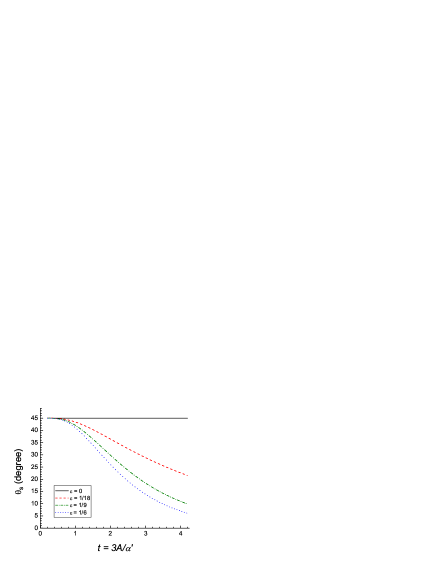
Figure 3: Plots for $\sin^{2}2\theta_{a}$ and $\theta_{s}$ as functions of $\varepsilon$ and $t$. The experimental data for atmospheric and solar mixings are $\sin^{2}2\theta_{\rm atm}>0.92$ at 90% CL and $\theta_{\rm sol}=(32\pm 3)^{\rm o}$.

Since in the weak coupling limit (large $t$), the couplings are given as $e^{-k{\rm Area}}$. One can easily see that the ratios $c/b$ and $b/a$ are exponentially damped in the weak coupling direction except for the two cases $\varepsilon=0$ (for $c/b$), $\frac{1}{6}$ (for $b/a$). In the strong coupling limit, all the triangles shrink and thus $a=b=c$. Thus, in the strong coupling limit, we have $\tan\theta_{a}=\sqrt{2}$ and $\tan\theta_{s}=1$ independent of $\varepsilon$. In this limit, however, due to the instanton corrections, the Yukawa couplings are blowing up and the effective theory is not reliable. When $t$ increases to $t\mathrel{\mathchoice{\lower 2.58334pt\vbox{\halign{$\m@th\displaystyle\hfil#\hfil$\cr>\crcr\sim\crcr}}}{\lower 2.58334pt\vbox{\halign{$\m@th\textstyle\hfil#\hfil$\cr>\crcr\sim\crcr}}}{\lower 2.58334pt\vbox{\halign{$\m@th\scriptstyle\hfil#\hfil$\cr>\crcr\sim\crcr}}}{\lower 2.58334pt\vbox{\halign{$\m@th\scriptscriptstyle\hfil#\hfil$\cr>\crcr\sim\crcr}}}}1$, the Yukawa couplings become $O(1)$ and the field theory can be in a perturbative region. In this region, $\theta_{a}$ always has the maximal mixing solution and $\theta_{s}$ starts to descent from the maximal value except for $\varepsilon=0$.

The mixing angles $\theta_{a,s}$ can be modified to $\theta_{a,s}^{l}$ due to the mixing angles in the light neutrino Majorana mass matrix. But, one can expect that the contribution from the Majorana matrix is small $\theta_{a,s}^{l}\simeq\theta_{a,s}$. We see that the solar and the atmospheric mixings can then be given by the moduli parameters. The observed qualitative features for neutrino oscillations, where the atmospheric mixing is almost maximal and the solar mixing is not maximal but large, can be interpreted geometrically when $t\sim 2$. This feature holds even for different intersection numbers.

We have shown in the previous section that the atmospheric mixing is almost the same as $\theta_{a}^{l}$ while the solar mixing can be modified as in Eq.(22) by $\theta_{13}$ and the MNSP phase. The calculated value of $\theta_{s}$ ($\varepsilon\neq 0$) is consistent with the observed solar mixing even if CP violation is maximal or small $\theta_{13}$ mixing. As shown in section 4, the observed data (for $\theta_{\rm sol}$ and $\theta_{\rm atm}$) are consistent with bi-maximal mixing $\theta_{a}=\theta_{s}=45^{\rm o}$ (which corresponds to $\varepsilon=0$ and $t=1.5$) when $U_{e3}$ is close to current experimental bound ($\theta_{13}<10^{\rm o}$ at 99% CL) and no CP violating phase in neutrino oscillation. We can distinguish two situations $\varepsilon=0$ or $\varepsilon\neq 0$ in the future long baseline experiments to measure $U_{e3}$ and the MNSP phase [27].

6 Conclusion

In this paper, we have studied Yukawa coupling structures in the intersecting D-brane models with the Pati-Salam gauge symmetry with extra $U(1)$ symmetries. The Yukawa matrices are almost rank 1 when the left- and right-handed matters are replicated on different tori. Because of the existence of $USp$ branes, four-point interaction can appear and the rank of the Yukawa matrices goes up due to the perturbation effects to the rank 1 matrices. With the almost rank 1 matrices, the observed quark and lepton mixings can be naturally reproduced. Especially, for the neutrino mixings, the bi-large and a small $\theta_{13}$ mixings can be naturally realized. Further, in the quark sector, $V_{cb}$ is naturally close to the strange/bottom quark mass ratio, and there exists a simple relation among the CKM mixing angles and a quark mass ratio. In the neutrino sector, the important prediction is that $U_{e3}$ is related to the 12 mixing in charged-lepton sector. Consequently, if the quark-lepton unification is realized simply, we predict $U_{e3}\simeq 0.05-0.15$ and almost the entire range of this prediction can be tested at future long baseline experiments [27]. We have also studied the geometrical meaning of the fact that the atmospheric mixing is almost maximal and the solar mixing is large but not maximal. This feature can arise when the Yukawa coupling is in the perturbative region. The results of the future long baseline experiments will be useful to shed light on geometrical interpretations.

We emphasize that the properties of fermion mixings which is reproduced from “almost rank 1” Yukawa matrices are model independent. These properties do not depend on how the rank of Yukawa matrices is raised. The crucial assumption is that the Yukawa coupling matrices are rank 1 plus small perturbations and the seesaw neutrino masses are type II dominant.

The “almost rank 1” matrices may be constructed in usual particle field theories, for example, by using Froggatt-Nielsen mechanism [28] with an appropriate flavor symmetry. Discrete flavor symmetry can also construct the rank 1 matrices. However, the rank 1 Yukawa matrices in the intersecting D-brane are not originating from symmetrical reason but from the geometrical configuration of the matter representation on tori. It is interesting that such patterns of fermion mixings in nature are naturally derived from a simple assumption in the context of string theory. The results can encourage us to understand the variety of quark and lepton masses and mixings in fundamental theories.

References

- [1] H. Fritzsch, Phys. Lett. B 70, 436 (1977); Phys. Lett. B 73, 317 (1978); Nucl. Phys. B 155, 189 (1979).
- [2] H. Georgi and C. Jarlskog, Phys. Lett. B 86, 297 (1979).
- [3] Y. Fukuda et al. [Super-Kamiokande Collaboration], Phys. Lett. B 433, 9 (1998) [hep-ex/9803006]; Phys. Lett. B 436, 33 (1998) [hep-ex/9805006]; Phys. Rev. Lett. 82, 2644 (1999) [hep-ex/9812014].
- [4] Q. R. Ahmad et al. [SNO Collaboration], Phys. Rev. Lett. 87, 071301 (2001) [nucl-ex/0106015]; Phys. Rev. Lett. 89, 011301 (2002) [nucl-ex/0204008]; K. Eguchi et al. [KamLAND Collaboration], Phys. Rev. Lett. 90, 021802 (2003) [hep-ex/0212021]; T. Araki et al. [KamLAND Collaboration], Phys. Rev. Lett. 94, 081801 (2005) [hep-ex/0406035].
- [5] M. Apollonio et al. [CHOOZ Collaboration], Phys. Lett. B 420, 397 (1998) [hep-ex/9711002]; Eur. Phys. J. C 27, 331 (2003) [hep-ex/0301017].
- [6] For minimal SO(10) models, T. Fukuyama and N. Okada, JHEP 0211, 011 (2002) [hep-ph/0205066]; B. Bajc, G. Senjanovic and F. Vissani, Phys. Rev. Lett. 90, 051802 (2003) [hep-ph/0210207]; H. S. Goh, R. N. Mohapatra and S. P. Ng, Phys. Lett. B 570, 215 (2003) [hep-ph/0303055]; B. Dutta, Y. Mimura and R. N. Mohapatra, Phys. Rev. Lett. 94, 091804 (2005) [hep-ph/0412105]; Phys. Rev. D 72, 075009 (2005) [hep-ph/0507319].
- [7] J. Polchinski, Phys. Rev. Lett. 75, 4724 (1995) [hep-th/9510017].
- [8] M. Berkooz, M. R. Douglas and R. G. Leigh, Nucl. Phys. B 480, 265 (1996) [hep-th/9606139]. H. Arfaei and M. M. Sheikh Jabbari, Phys. Lett. B 394, 288 (1997) [hep-th/9608167].
- [9] R. Blumenhagen, L. Goerlich, B. Kors and D. Lust, JHEP 0010, 006 (2000) [hep-th/0007024]; R. Blumenhagen, B. Kors and D. Lust, JHEP 0102, 030 (2001) [hep-th/0012156]; G. Aldazabal, S. Franco, L. E. Ibanez, R. Rabadan and A. M. Uranga, JHEP 0102, 047 (2001) [hep-ph/0011132].
- [10] J. C. Pati and A. Salam, Phys. Rev. D 10, 275 (1974).
- [11] D. Cremades, L. E. Ibanez and F. Marchesano, JHEP 0307, 038 (2003) [hep-th/0302105]; JHEP 0405, 079 (2004) [hep-th/0404229].
- [12] M. Cvetic and I. Papadimitriou, Phys. Rev. D 68, 046001 (2003) [hep-th/0303083]; S. A. Abel and A. W. Owen, Nucl. Phys. B 663, 197 (2003) [hep-th/0303124]; Nucl. Phys. B 682, 183 (2004) [hep-th/0310257]; D. Lust, P. Mayr, R. Richter and S. Stieberger, Nucl. Phys. B 696, 205 (2004) [hep-th/0404134]; S. A. Abel and B. W. Schofield, JHEP 0506, 072 (2005) [hep-th/0412206].
- [13] T. Higaki, N. Kitazawa, T. Kobayashi and K. j. Takahashi, Phys. Rev. D 72, 086003 (2005) [hep-th/0504019].
- [14] M. Cvetic, G. Shiu and A. M. Uranga, Phys. Rev. Lett. 87, 201801 (2001) [hep-th/0107143]; Nucl. Phys. B 615, 3 (2001) [hep-th/0107166]; D. Cremades, L. E. Ibanez and F. Marchesano, JHEP 0207, 022 (2002) [hep-th/0203160]; M. Cvetic, P. Langacker and G. Shiu, Nucl. Phys. B 642, 139 (2002) [hep-th/0206115]; G. Honecker and T. Ott, Phys. Rev. D 70, 126010 (2004) [hep-th/0404055]; C. Kokorelis, hep-th/0410134; C. M. Chen, T. Li and D. V. Nanopoulos, hep-th/0509059; G. K. Leontaris and J. Rizos, hep-ph/0510230.
- [15] C. Kokorelis, JHEP 0208, 018 (2002) [hep-th/0203187]; J. R. Ellis, P. Kanti and D. V. Nanopoulos, Nucl. Phys. B 647, 235 (2002) [hep-th/0206087]; C. M. Chen, G. V. Kraniotis, V. E. Mayes, D. V. Nanopoulos and J. W. Walker, Phys. Lett. B 611, 156 (2005) [hep-th/0501182]; Phys. Lett. B 625, 96 (2005) [hep-th/0507232].
- [16] M. Cvetic, T. Li and T. Liu, Nucl. Phys. B 698, 163 (2004) [hep-th/0403061].
- [17] F. Marchesano and G. Shiu, Phys. Rev. D 71, 011701 (2005) [hep-th/0408059]; JHEP 0411, 041 (2004) [hep-th/0409132]. Phys. Rev. D 71, 106008 (2005) [hep-th/0501041].
- [18] N. Chamoun, S. Khalil and E. Lashin, Phys. Rev. D 69, 095011 (2004) [hep-ph/0309169].
- [19] S. A. Abel, O. Lebedev and J. Santiago, Nucl. Phys. B 696, 141 (2004) [hep-ph/0312157].
- [20] N. Kitazawa, Nucl. Phys. B 699, 124 (2004) [hep-th/0401096]; N. Kitazawa, T. Kobayashi, N. Maru and N. Okada, Eur. Phys. J. C 40, 579 (2005) [hep-th/0406115]; T. Noguchi, hep-ph/0410302.
- [21] For a reivew, R. Blumenhagen, M. Cvetic, P. Langacker and G. Shiu, hep-th/0502005.
- [22] G. Aldazabal, S. Franco, L. E. Ibanez, R. Rabadan and A. M. Uranga, J. Math. Phys. 42, 3103 (2001) [hep-th/0011073].
- [23] M. Cvetic, P. Langacker, T. j. Li and T. Liu, Nucl. Phys. B 709, 241 (2005) [hep-th/0407178].
- [24] M. Cvetic, P. Langacker and J. Wang, Phys. Rev. D 68, 046002 (2003) [hep-th/0303208].
- [25] P. Minkowski, Phys. Lett. B 67, 421 (1977); T. Yanagida, in proc. of KEK workshop, eds. O. Sawada and S. Sugamoto (Tsukuba, 1979); M. Gell-Mann, P. Ramond and R. Slansky, in Supergravity, eds. P. van Nieuwenhuizen and D. Z. Freedman (North-Holland, Amsterdam, 1979); R. N. Mohapatra and G. Senjanović, Phys. Rev. Lett. 44, 912 (1980).
- [26] S. Eidelman et al. [Particle Data Group], Phys. Lett. B 592, 1 (2004).
- [27] K. Anderson et al., hep-ex/0402041; Y. Itow et al., hep-ex/0106019; Y. Hayato [T2K Collaboration], Nucl. Phys. Proc. Suppl. 147, 9 (2005); F. Dalnoki-Veress [Double-Chooz Project Collaboration], hep-ex/0406070; D. S. Ayres et al. [NOvA Collaboration], hep-ex/0503053; M. Kuze [KASKA Collaboration], Nucl. Phys. Proc. Suppl. 149, 160 (2005) [hep-ex/0502002].
- [28] C. D. Froggatt and H. B. Nielsen, Nucl. Phys. B 147, 277 (1979).