We study the single spin asymmetry (SSA) for the pion production with large transverse momentum $p_{T}$ in semi-inclusive deep inelastic scattering $ep^{\uparrow}\to e\pi X$. We derive the twist-3 cross section formula for SSA, focussing on the soft-gluon-pole contributions associated with the twist-3 distribution for the nucleon and with the twist-3 fragmentation function for the pion. We present a simple estimate of the asymmetries due to each twist-3 effect from nucleon and pion, respectively, by fixing the overall strength of the relevant nonperturbative quantities by the data on the SSA $A_{N}$ in $p^{\uparrow}p\to\pi X$ collision.

1 Introduction

Single transverse spin asymmetries (SSAs) in the strong interaction have a long history since 70s and 80s when the large asymmetries were observed in $pp\to\Lambda^{\uparrow}X$ [1] and $p^{\uparrow}p\to\pi X$ [2] in the forward direction. These data triggered lots of theoretical activities to clarify the mechanism of the asymmetries [3]. Experimentally measurements of SSA at higher energies in $pp$ collisions have been performed at RHIC [4, 5, 6], and SSAs in semi-inclusive deep inelastic scattering (SIDIS) have been also reported [7, 8]. The SSA is a so-called “naively T-odd” observable proportional to $(\vec{p}\times\vec{q})\cdot\vec{S}_{\perp}$, and time-reversal invariance in QCD implies that it only occurs from the interference between the amplitudes which have different phases. In the literature, two QCD mechanisms have been used for describing the observed large SSAs. One is based on the use of so-called “T-odd” distribution and fragmentation functions which have explicit intrinsic transverse momentum $\vec{k}_{\perp}$ of partons inside hadrons [9, 10]. This mechanism describes the SSA as a leading twist effect in the region of small transverse momentum $p_{T}$ of the produced hadron. Factorization formula with the use of $k_{\perp}$ dependent parton distribution functions and fragmentation functions has been extended to SIDIS [11], applying the method used for $e^{+}e^{-}$ annihilation [12] and the Drell-Yan process [13], and the universality property of those $k_{\perp}$-dependent functions have been examined in great details  [14, 15, 16, 17, 18]. Phenomenological applications of the “T-odd” functions have been also performed to interprete the existing data for SSAs [19].

The other mechanism describes the SSA as a twist-3 effect in the collinear factorization, and is suited for describing SSA in the large $p_{T}$ region [20, 21, 22, 23, 24, 25, 26]. In this framework, SSA is connected to particular quark-gluon correlation functions on the lightcone. This method has been extensively applied to SSA in $pp$ collisions, such as direct photon production $p^{\uparrow}p\to\gamma X$ [21], pion production $p^{\uparrow}p\to\pi X$ [22, 23, 26], and the hyperon polarization $pp\to\Lambda^{\uparrow}X$ [24] etc. Although the above two mechanisms describe SSA in different kinematic regions, it has been known that a soft-gluon pole function appearing in the twist-3 mechanism is connected to a $\vec{k}_{\perp}$ moment of a “T-odd” function [16]. More recently, the authors of ref. [27] showed that the two mechanisms give the identical SSA for the Drell-Yan process in the intermediate $p_{T}$ region, unifying the two mechanisms.

In this paper, we study the SSA for large-$p_{T}$ pion production in SIDIS, $ep^{\uparrow}\to e\pi X$.  The QCD factorization tells us that the cross section for this process is generically expressed as convolution of three quantities, a distribution function for the transversely polarized nucleon, a fragmentation function for the pion, and a partonic hard cross section. In the framework of the collinear factorization, the SSAs at the leading order in QCD perturbation theory require participation of an additional, coherent gluon into the partonic subprocess [20], and the corresponding gluon field can be generated from either the nucleon or the pion, as shown in (a) and (b) of Fig. 1, respectively. These two contributions give rise to the following twist-3 cross section, denoting respectively as the (A) and (B) terms:

$$({\rm A}) G_{F}(x_{1},x_{2})\otimes D(z)\otimes\widehat{\sigma}_{\rm A},$$

$$({\rm B}) \delta q(x)\otimes\widehat{E}_{F}(z_{1},z_{2})\otimes\widehat{\sigma}_{\rm B},$$ (1)

where $G_{F}(x_{1},x_{2})$ and $\widehat{E}_{F}(z_{1},z_{2})$ are, respectively, the twist-3 distribution function for the transversely polarized nucleon and the twist-3 fragmentation function for the pion; the definition of these twist-3 functions is given in (2) and (8) below. In (1) there also appear the familiar twist-2 functions: $\delta q(x)$ is the quark transversity distribution of the nucleon, and $D(z)$ is the usual quark/gluon fragmentation function for the pion. $\widehat{\sigma}_{\rm A,B}$ are the partonic hard cross sections, and we present their explicit formula in QCD perturbation theory. We note that both distribution and fragmentation functions in the (A) term of (1) are chiral-even, while both of those functions in the (B) term are chiral-odd. Accordingly, we have only one diagram in Fig. 1(b) relevant to the (B) term. We also note that there exist purely gluonic twist-3 distributions for the transversely polarized nucleon which can contribute to the (A) term in (1) [29]. The study of this term is beyond the scope of the present work, and we shall restrict ourselves to the kinematic region where the contribution from the quark-gluon correlation is expected to be dominant compared with that from the three-gluon correlation.

It has been already shown that the twist-3 functions $G_{F}$ and $\widehat{E}_{F}$ appearing in (1) can potentially be important sources for the large asymmetry $A_{N}$ observed at large $x_{F}$ for $p^{\uparrow}p\to\pi X$ [22, 26]. Therefore, our interest here is to study how the above effects (A) and (B) contribute to the SSA in SIDIS, if the overall strengths of the relevant twist-3 nonperturbative quantities $G_{F}(x_{1},x_{2})$, $\widehat{E}_{F}(z_{1},z_{2})$, as well as the transversity $\delta q(x)$, are determined so as to reproduce $A_{N}$ in $pp$ collisions [2, 4].

The remainder of this paper is organized as follows: In section 2, we present definition of the twist-3 distribution and fragmentation functions necessary in our analysis. In section 3, after a brief description of the kinematics for SIDIS, we present the polarized cross section formula for the two contributions in (1), focussing on the soft-gluon-pole contributions. Azimuthal asymmetries from each contribution are discussed in detail and their numerical estimate is also presented. A brief summary is given in section 5. Appendix provides an explicit relation between the different definitions for the twist-3 distribution functions.

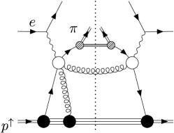
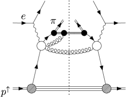
(a)                                                                      (b)

Figure 1: (a) Contribution to $ep^{\uparrow}\to e\pi X$ from the twist-3 distribution $G_{F}$; in the left (right) diagram, a quark (gluon) fragments into $\pi+$anything. (b) Contribution to $ep^{\uparrow}\to e\pi X$ from the twist-3 fragmentation function $\widehat{E}_{F}$. The white circles represent partonic hard scatterings. Mirror diagrams obtained by the interchange between left and right of the cut also contribute.

2 Twist-3 quark-gluon correlation functions

We first discuss the definition and basic properties of the twist-3 distributions for the transversely polarized nucleon, which are relevant to $ep^{\uparrow}\to e\pi X$. As shown in (a) of Fig. 1, these distributions actually represent the quark-gluon correlation inside the nucleon. For the transversely polarized nucleon with momentum $p^{\mu}$ and spin $S_{\perp}^{\mu}$, there are two independent twist-3 quark-gluon correlation functions which are defined as nucleon matrix element of nonlocal lightcone operator  [21, 22, 30]

$$\int{d\lambda\over 2\pi}\int{d\mu\over 2\pi}e^{i\lambda x_{1}}e^{i\mu(x_{2}-x_{1})}\langle p\ S_{\perp}|\bar{\psi}_{j}(0)[0,\mu n]{gF^{\alpha\beta}(\mu n)n_{\beta}}[\mu n,\lambda n]\psi_{i}(\lambda n)|p\ S_{\perp}\rangle$$

$$\qquad={M_{N}\over 4}\left(\hbox to0.0pt{/\hss}{\mkern-1.0mup}\right)_{ij}\epsilon^{\alpha pnS_{\perp}}{G_{F}(x_{1},x_{2})}+i{M_{N}\over 4}\left(\gamma_{5}\hbox to0.0pt{/\hss}{\mkern-1.0mup}\right)_{ij}S_{\perp}^{\alpha}{\widetilde{G}_{F}(x_{1},x_{2})}+\cdots,$$ (2)

where $\psi$ is the quark field, $F^{\alpha\beta}$ is the gluon field strength tensor, $n^{\mu}$ is the light-like vector ($n^{2}=0$) with $p\cdot n=1$, $\epsilon^{\alpha pnS_{\perp}}=\epsilon^{\alpha\lambda\mu\nu}p_{\lambda}n_{\mu}S_{\perp\nu}$ with $\epsilon_{0123}=1$, and the spin vector satisfies $S_{\perp}^{2}=-1$, $S_{\perp}\cdot p=S_{\perp}\cdot n=0$. $[\mu n,\lambda n]={\rm P}\exp\left[ig\int_{\lambda}^{\mu}dtn\cdot A(tn)\right]$ represents the gauge-link which guarantees gauge invariance of the nonlocal lightcone operator, and “$\cdots$” denotes twist-4 or higher-twist distributions. The correlation functions $G_{F}(x_{1},x_{2})$, $\widetilde{G}_{F}(x_{1},x_{2})$ are defined as dimensionless, and the nucleon mass $M_{N}$ in the RHS of (2) represents a natural scale for chiral-symmetry breaking. Each correlation function depends on the two variables $x_{1}$ and $x_{2}$, where $x_{1}$ and $x_{2}-x_{1}$ are the fractions of the lightcone momentum carried by the quark and the gluon, respectively, which are outgoing from the nucleon. From P- and T-invariance in QCD, one can show the symmetry properties

$$G_{F}(x_{1},x_{2})=G_{F}(x_{2},x_{1}),\qquad\widetilde{G}_{F}(x_{1},x_{2})=-\widetilde{G}_{F}(x_{2},x_{1}),$$ (3)

and from hermiticity both $G_{F}(x_{1},x_{2})$ and $\widetilde{G}_{F}(x_{1},x_{2})$ are real functions. These two correlation functions $G_{F}(x_{1},x_{2})$ and $\widetilde{G}_{F}(x_{1},x_{2})$ constitute a complete set of the twist-3 quark-gluon correlation functions for the transversely polarized nucleon (see e.g. ref. [30] for a concise discussion).

In the literature, however, another set of twist-3 quark-gluon correlation functions are also used [21, 22]: Replacing the field strength $gF^{\alpha\beta}(\mu n)n_{\beta}$ in the LHS in (2) by the transverse components of the covariant derivative, $D_{\perp}^{\alpha}(\mu n)=\partial_{\perp}^{\alpha}-igA_{\perp}^{\alpha}(\mu n)$, the same Lorentz decomposition in the RHS defines the two twist-3 distributions $G_{D}(x_{1},x_{2})$ and $\widetilde{G}_{D}(x_{1},x_{2})$, in place of $G_{F}(x_{1},x_{2})$ and $\widetilde{G}_{F}(x_{1},x_{2})$, respectively. Physical meaning as well as the basic properties of $G_{D}(x_{1},x_{2})$ and $\widetilde{G}_{D}(x_{1},x_{2})$ are similar to $G_{F}(x_{1},x_{2})$ and $\widetilde{G}_{F}(x_{1},x_{2})$, except that P- and T-invariance implies $G_{D}(x_{1},x_{2})=-G_{D}(x_{2},x_{1})$, $\widetilde{G}_{D}(x_{1},x_{2})=\widetilde{G}_{D}(x_{2},x_{1})$.

Overcomplete set of four twist-3 correlation functions $G_{F}(x_{1},x_{2})$, $\widetilde{G}_{F}(x_{1},x_{2})$, $G_{D}(x_{1},x_{2})$, and $\widetilde{G}_{D}(x_{1},x_{2})$ for transversely polarized nucleon has been conveniently used on a case-by-case basis to express the cross section formula in the literature. Here we present an explicit relation between the “$F$-type” distributions ($G_{F}(x_{1},x_{2}),\widetilde{G}_{F}(x_{1},x_{2})$) and the “$D$-type” functions ($G_{D}(x_{1},x_{2}),\widetilde{G}_{D}(x_{1},x_{2})$). For this purpose, we refer to the operator identity with manifest gauge invariance,

$$D^{\alpha}(\mu n)[\mu n,\lambda n]=i\int_{\lambda}^{\mu}dt[\mu n,tn]gF^{\alpha\beta}(tn)n_{\beta}[tn,\lambda n]+[\mu n,\lambda n]D^{\alpha}(\lambda n),$$ (4)

which relates (2) with the corresponding matrix element for the $D$-type distributions. One then obtains

$$G_{D}(x_{1},x_{2}) = P{1\over x_{1}-x_{2}}G_{F}(x_{1},x_{2}),$$ (5)

$$\widetilde{G}_{D}(x_{1},x_{2}) = \delta(x_{1}-x_{2})\widetilde{g}(x_{1})+P{1\over x_{1}-x_{2}}\widetilde{G}_{F}(x_{1},x_{2}),$$ (6)

where $P$ denotes the principal value, and

$$\widetilde{g}(x)=\frac{-i}{M_{N}}\int{d\lambda\over 2\pi}e^{i\lambda x}\langle p\ S_{\perp}|\bar{\psi}(0)[0,\lambda n]\gamma_{5}{\mathchoice{\c@ncel\displaystyle{\mkern-1.0mun}}{\c@ncel\textstyle{\mkern-1.0mun}}{\c@ncel\scriptstyle{\mkern-1.0mun}}{\c@ncel\scriptscriptstyle{\mkern-1.0mun}}}S_{\perp}\cdot D(\lambda n)\psi(\lambda n)|p\ S_{\perp}\rangle$$

$$+ \!\!\!\!{1\over 2M_{N}}\int{d\lambda\over 2\pi}e^{i\lambda x}\int_{-\infty}^{\infty}d\mu\,\epsilon(\mu-\lambda)\,\langle p\ S_{\perp}|\bar{\psi}(0)[0,\lambda n]\gamma_{5}{\mathchoice{\c@ncel\displaystyle{\mkern-1.0mun}}{\c@ncel\textstyle{\mkern-1.0mun}}{\c@ncel\scriptstyle{\mkern-1.0mun}}{\c@ncel\scriptscriptstyle{\mkern-1.0mun}}}gF^{S_{\perp}n}(\mu n)[\mu n,\lambda n]\psi(\lambda n)|p\ S_{\perp}\rangle,$$

with $\epsilon(\mu-\lambda)=2\theta(\mu-\lambda)-1$. In the RHS of (5), the term proportional to $\delta(x_{1}-x_{2})$ vanishes due to the anti-symmetry of $G_{D}(x_{1},x_{2})$ as stated above. In Appendix, we demonstrate that $\widetilde{g}(x)$ can be reexpressed in terms of the $F$-type distributions $G_{F}(x_{1},x_{2})$ and $\widetilde{G}_{F}(x_{1},x_{2})$, and the twist-2 quark helicity distribution $\Delta q(x)$ of the nucleon. The relations (5) and (6) show that the $D$-type functions are more singular than the $F$-type functions at the soft gluon point $x_{1}=x_{2}$, while they are proportional to each other for $x_{1}\neq x_{2}$. In our analysis for $ep^{\uparrow}\to e\pi X$ below, we assume that there is no singularity in the $F$-type functions, in particular, that $G_{F}(x_{1},x_{2})$ is finite at $x_{1}=x_{2}$ ($\widetilde{G}_{F}(x_{1},x_{1})=0$, due to (3)).

Similarly to the distributions, one can also construct the twist-3 fragmentation function for the pion with momentum $\ell$ as [25, 16, 26]

$${1\over N_{c}}\sum_{X}\int{d\lambda\over 2\pi}\int{d\mu\over 2\pi}e^{-i{\lambda\over z_{1}}}e^{-i\mu({1\over z_{2}}-{1\over z_{1}})}\langle 0|[-\infty w,0]\psi_{i}(0)|\pi(\ell)X\rangle$$

$$\qquad\qquad\qquad\times\langle\pi(\ell)X|\bar{\psi}_{j}(\lambda w)[\lambda w,\mu w]{gF^{\alpha\beta}(\mu w)w_{\beta}}[\mu w,-\infty w]|0\rangle$$

$$\qquad={{M_{N}}\over 2z_{2}}\left(\gamma_{5}\hbox to0.0pt{/\hss}{\mkern-1.0mu\ell}\gamma_{\nu}\right)_{ij}\epsilon^{\nu\alpha w\ell}{\widehat{E}_{F}(z_{1},z_{2})}+\cdots,$$ (8)

where we introduced the light-like vector $w$ by the relation $\ell\cdot w=1$, and “$\cdots$” denotes twist-4 or higher, and we again use the nucleon mass $M_{N}$ as a generic QCD mass scale in order to define $\widehat{E}_{F}(z_{1},z_{2})$ as dimensionless. A fragmentation function obtained by shifting the field strength ${gF^{\alpha\beta}(\mu n)w_{\beta}}$ from the matrix element $\langle\pi(\ell)X|\cdots|0\rangle$ to $\langle 0|\cdots|\pi(\ell)X\rangle$ is expressed in terms of $\widehat{E}_{F}^{*}(z_{2},z_{1})$. Unlike (3) for the twist-3 distributions, time reversal invariance does not bring any constraint on the symmetry properties of the twist-3 fragmentation functions. As in the case for the twist-3 distribution, we can also define another twist-3 quark-gluon fragmentation function $\widehat{E}_{D}(z_{1},z_{2})$, replacing ${gF^{\alpha\beta}(\mu w)w_{\beta}}$ by the covariant derivative $\overleftarrow{D}_{\perp}^{\alpha}(\mu w)$ in (8) [31]. The relation between $\widehat{E}_{D}(z_{1},z_{2})$ and $\widehat{E}_{F}(z_{1},z_{2})$ can be easily obtained by using the identity (4) as

$$\widehat{E}_{D}(z_{1},z_{2})=\delta\left({1\over z_{1}}-{1\over z_{2}}\right)\widetilde{e}(z_{1})+P{1\over(1/z_{1})-(1/z_{2})}\widehat{E}_{F}(z_{1},z_{2}),$$ (9)

where

$$\widetilde{e}(z) = {z\over 4M_{N}}{1\over N_{c}}\sum_{X}\int{d\lambda\over 2\pi}\,e^{-i\lambda/z}\langle 0|[-\infty w,0]\gamma^{\nu}\hbox to0.0pt{/\hss}{\mkern-1.0muw}\gamma_{5}\psi(0)|\pi(\ell)X\rangle$$ (10)

$$\qquad\times\langle\pi(\ell)X|\bar{\psi}(\lambda w)\overleftarrow{D}^{\alpha}(\lambda w)[\lambda w,-\infty w]|0\rangle\epsilon_{\nu\alpha}^{\ \ \,w\ell}$$

$$-{iz\over 8M_{N}}{1\over N_{c}}\sum_{X}\int{d\lambda\over 2\pi}\,e^{-i\lambda/z}\int_{-\infty}^{\infty}d\mu\,\epsilon(\mu-\lambda)\langle 0|[-\infty w,0]\gamma^{\nu}\hbox to0.0pt{/\hss}{\mkern-1.0muw}\gamma_{5}\psi(0)|\pi(\ell)X\rangle$$

$$\qquad\times\langle\pi(\ell)X|\bar{\psi}(\lambda w)[\lambda w,\mu w]g{F}^{\alpha w}(\mu w)[\mu w,-\infty w]|0\rangle\epsilon_{\nu\alpha}^{\ \ \,w\ell}.$$

Here we emphasize again that $\widehat{E}_{D}(z_{1},z_{2})$ is more singular compared to $\widehat{E}_{F}(z_{1},z_{2})$ at $z_{1}=z_{2}$, while they are proportional to each other for $z_{1}\neq z_{2}$. As will be discussed in the next section, the cross section for $ep^{\uparrow}\to e\pi X$ receives important contribution from the “soft gluon point”, $x_{1}=x_{2}$ or $z_{1}=z_{2}$, of the twist-3 functions defined above. We thus use the corresponding $F$-type functions to express those contributions in the cross section. Other terms which receive contributions with $x_{1}\neq x_{2}$, $z_{1}\neq z_{2}$ are expressed in terms of either $D$-type or $F$-type functions without any subtlety.

3 Single spin asymmetry for $ep^{\uparrow}\to e\pi X$

3.1 Kinematics

Here we present a brief description of the kinematics for the SIDIS, $e(k)+p(p,S_{\perp})\to e(k^{\prime})+\pi(\ell)+X$. (See refs. [32, 33] for the detail.) We have five independent Lorentz invariants, $S_{ep},x_{bj},Q^{2},z_{f}$, and $q_{T}^{2}$. The center of mass energy squared, $S_{ep}$, for the initial electron and the proton is

$$S_{ep}=(p+k)^{2}\simeq 2p\cdot k\;,$$ (11)

ignoring masses. The conventional DIS variables are defined in terms of the virtual photon momentum $q=k-k^{\prime}$ as

$$x_{bj}={Q^{2}\over 2p\cdot q}\;,\qquad Q^{2}=-q^{2}=-(k-k^{\prime})^{2}.$$ (12)

For the final-state pion, we introduce the scaling variable

$$z_{f}={p\cdot\ell\over p\cdot q}\;.$$ (13)

Finally, we define the “transverse” component of $q$, which is orthogonal to both $p$ and $\ell$:

$$q_{t}^{\mu}=q^{\mu}-{\ell\cdot q\over p\cdot\ell}p^{\mu}-{p\cdot q\over p\cdot\ell}\ell^{\mu}\;.$$ (14)

$q_{t}$ is a space-like vector, and we denote its magnitude by

$$q_{T}=\sqrt{-q_{t}^{2}}\;.$$ (15)

To completely specify the kinematics, we need to choose a reference frame. We shall work in the so-called hadron frame [32], which is the Breit frame of the virtual photon and the initial proton:

$$q^{\mu} = (0,0,0,-Q)\;,$$ (16)

$$p^{\mu} = \left({Q\over 2x_{bj}},0,0,{Q\over 2x_{bj}}\right)\;.$$ (17)

Further, in this frame the outgoing pion is taken to be in the $xz$ plane:

$$\ell^{\mu}={z_{f}Q\over 2}\left(1+{q_{T}^{2}\over Q^{2}},{2q_{T}\over Q},0,{q_{T}^{2}\over Q^{2}}-1\right)\;.$$ (18)

As one can see, the transverse momentum of the pion is in this frame given by $\ell_{T}=z_{f}q_{T}$. This is true for any frame in which the 3-momenta of the virtual photon and the initial proton are collinear. By introducing the angle $\phi$ between the hadron plane and the lepton plane, the lepton momentum can be parameterized as

$$k^{\mu}={Q\over 2}\left(\cosh\psi,\sinh\psi\cos\phi,\sinh\psi\sin\phi,-1\right)\;,$$ (19)

and one finds

$$\cosh\psi={2x_{bj}S_{ep}\over Q^{2}}-1\;.$$ (20)

We parameterize the transverse spin vector of the initial proton $S_{\perp}^{\mu}$ as

$$S^{\mu}_{\perp}=(0,\cos\Phi_{S},\sin\Phi_{S},0),$$ (21)

where $\Phi_{S}$ represents the azimuthal angle of $\vec{S}_{\perp}$ measured from the hadron plane. With the above definition, the cross section for $ep^{\uparrow}\to e\pi X$ can be expressed in terms of $S_{ep}$, $x_{bj}$, $Q^{2}$, $z_{f}$, $q_{T}^{2}$, $\phi$ and $\Phi_{S}$ in the hadron frame. Note that $\phi$ and $\Phi_{S}$ are invariant under boosts in the $\vec{q}$-direction, so that the cross section presented below is the same in any frame where $\vec{q}$ and $\vec{p}$ are collinear.

3.2 Twist-3 polarized cross section

We now proceed to derive the cross section for $ep^{\uparrow}\to e\pi X$, applying the method developed in [21, 22]. We use Feynman gauge in the actual calculation. In this framework, the phase necessary for SSAs is provided from the partonic hard cross section. To illustrate, consider the diagrams in the first line of Fig. 2(a), which are some of the leading order contributions in perturbation theory corresponding to Fig. 1(a). These diagrams involve the coherent gluon from the nucleon, participating in the partonic hard scattering. After the collinear expansion in the transverse momenta $k_{\perp}$ of the partons inside nucleon to $O(k_{\perp})$, the “external” partons for the partonic hard cross section are collinear to their parent hadron. Denoting the momenta of the external quark lines on the LHS of the cut as $x_{1}p$ and $\ell/z$, and the momentum of the coherent gluon as $(x_{2}-x_{1})p$, where $x_{1},x_{2}$, and $z$ are the corresponding momentum fractions to be integrated over, the parton propagator coupled to the coherent gluon gives a factor $1/(x_{1}-x_{2}+i\varepsilon)$. Then the integration for the parton momentum fraction produces the phase from the pole contribution at the soft gluon point $x_{1}=x_{2}$ (soft-gluon-pole (SGP)) [21], which may be evaluated through the distribution identity

$${1\over x_{1}-x_{2}+i\varepsilon}=P{1\over x_{1}-x_{2}}-i\pi\delta(x_{1}-x_{2}).$$ (22)

It is straightforward to see that another propagator in the LHS of the cut in the first and third diagrams in the first line in Fig. 2(a) is proportional to $1/(x_{1}-i\varepsilon)=P(1/x_{1})+i\pi\delta(x_{1})$, which produces the soft-fermion-pole (SFP) contribution at $x_{1}=0$ [21]. Similarly another propagator in the LHS of the cut in the second and fourth diagrams in the first line in Fig. 2(a) is proportional to $1/(x_{1}-x_{bj}+i\varepsilon)=P\{1/(x_{1}-x_{bj})\}-i\pi\delta(x_{1}-x_{bj})$, which produces the hard-pole (HP) contribution at $x_{1}=x_{bj}$ [34]. There are other leading order diagrams of the type of Fig. 1(a), which receive the SFP and HP contributions. As anticipated, the SGP contributions, as well as the SFP and HP contributions, are eventually associated with the quark-gluon correlation beyond twist-2, and are expressed by a complete set of the twist-3 quark-gluon correlation functions, $G_{F}(x_{1},x_{2})$ and $\widetilde{G}_{F}(x_{1},x_{2})$ of (2). From the symmetry (3) under $x_{1}\leftrightarrow x_{2}$, $\widetilde{G}_{F}(x_{1},x_{2})$ does not contribute to the SGP at $x_{1}=x_{2}$. On the other hand, as a result of the collinear expansion, some of the SGP contributions appear with the derivative like ${d\over dx}G_{F}(x,x)$, while SFP and HP contributions do not appear with such derivative. In the large $x$ region, one has $|x{d\over dx}G_{F}(x,x)|\gg|G_{F}(x,x)|$, since $G_{F}(x,x)$ is expected to behave as $G_{F}(x,x)\sim(1-x)^{\beta}$ ($\beta>0$). Accordingly, it is justified to keep only the derivative terms with ${d\over dx}G_{F}(x,x)$ in the SGP contributions for the case where only large $x$ region is relevant.

Similarly, the diagrams in Fig. 2(b), which are some of the leading order contributions in perturbation theory corresponding to Fig. 1(b), also receive the pole contributions. After the collinear expansion, the quark momenta entering and leaving the pion fragmentation function can be parameterized as $\ell/z_{1}$ and $\ell/z_{2}$, respectively. In this case, the pole contributions, which give the phase for SSA, come from the SGP contribution at $z_{1}=z_{2}$ and the HP contribution at $z_{1}=z_{f}(1-q_{T}^{2}/Q^{2})$. But there appears no SFP contribution, since $1/z_{i}\neq 0$ ($i=1,\ 2$). Again, some of the SGP contributions appear with the derivative of $\widehat{E}_{F}$, while no derivative appears for the HP contributions. 

In our present study, we shall focus on the derivative terms of the SGP contributions following the previous studies [22, 23, 24, 26]. This approximation should be valid if either $x_{bj}$ or $z_{f}$ is large, where the main contribution is from large-$x$ and large-$z$ regions (see the cross section formula derived below). Also, physically, one expects that the SFP and HP contributions are suppressed compared to the SGP contributions, because there may be lots of soft gluons in the hadrons; in particular, for the SFP contributions, not much soft fermions are expected to exist in a hadron.

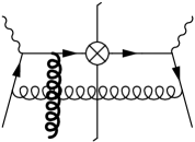
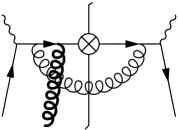
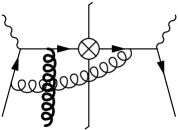
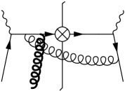
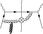
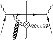
(a)

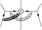
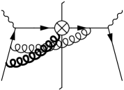
(b)

Figure 2: (a) and (b) represent Feynman diagrams which give rise to SGP contributions for $G_{F}$ and $\widehat{E}_{F}$, respectively. $\otimes$ denotes fragmentation insertions. In both cases, mirror diagrams also contribute.

The diagrams which receive the SGP contributions of the type (A) in (1) are shown in Fig. 2(a). By including only the derivative terms of the SGP contribution, one obtains the spin-dependent differential cross section as

$${d^{5}\sigma^{({\rm A})}\over dx_{bj}dQ^{2}dz_{f}dq_{T}^{2}d\phi} = {\alpha_{em}^{2}\alpha_{s}\over 8\pi x_{bj}^{2}S_{ep}^{2}Q^{2}}\left({M_{N}q_{T}\pi\over Q^{2}}\right)x_{bj}^{2}\sin\Phi_{S}\sum_{a}e_{a}^{2}\int_{x_{min}}^{1}\,{dx\over x}\int_{z_{min}}^{1}\,{dz\over z}\,$$

$$\times \left({d\over dx}{G}_{F}^{a}(x,x)\right)\left(D_{a}(z)C_{a}\widehat{\sigma}_{qq}^{\rm A}+D_{g}(z)C_{g}\widehat{\sigma}_{gq}^{\rm A}\right){\widehat{z}\over(1-\widehat{z})^{2}}\delta(x-x_{0}),$$

(23)

where $\alpha_{em}=e^{2}/4\pi$ is the QED coupling constant, and we have introduced the variables

$$\widehat{x}={x_{bj}\over x}\;,\qquad\widehat{z}={z_{f}\over z}\;,$$ (24)

$$x_{min}=x_{bj}\left(1+{z_{f}\over 1-z_{f}}{q_{T}^{2}\over Q^{2}}\right)\;,\qquad z_{min}=z_{f}\left(1+{x_{bj}\over 1-x_{bj}}{q_{T}^{2}\over Q^{2}}\right)\;,$$ (25)

$$x_{0}=x_{bj}\left(1+{\widehat{z}\over 1-\widehat{z}}{q_{T}^{2}\over Q^{2}}\right).$$ (26)

In (23), $G_{F}^{a}$ denotes the twist-3 distribution for the quark flavor $a$ defined in (2), $D_{a}(z)/D_{g}(z)$ is the unpolarized quark (flavor $a$)/gluon fragmentation function for the pion, and $e_{a}$ is the electric charge for the quark flavor $a$. The color factor $C_{a,g}$ is defined as $C_{q}=C_{F}-N_{c}/2=-1/(2N_{c})$ for quark and $C_{\bar{q}}=1/(2N_{c})$ for anti-quark, and $C_{g}=N_{c}/2$ for gluon. The partonic hard cross section $\widehat{\sigma}_{jq}^{\rm A}$ ($j=q,\ g$) in (23) is written as

$$\widehat{\sigma}_{jq}^{\rm A}=\left(1+\cosh^{2}\psi\right)\,\widehat{\sigma}^{1}_{jq}-2\widehat{\sigma}_{jq}^{2}-\sinh 2\psi\cos\phi\,\widehat{\sigma}^{3}_{jq}+\sinh^{2}\psi\cos 2\phi\,\widehat{\sigma}^{4}_{jq},\qquad(j=q,g)$$ (27)

where

$$\widehat{\sigma}^{1}_{qq} = 2\widehat{x}\widehat{z}\left\{{1\over Q^{2}q_{T}^{2}}\left({Q^{4}\over\widehat{x}^{2}\widehat{z}^{2}}+\left(Q^{2}-q_{T}^{2}\right)^{2}\right)+6\right\}\;,$$

$$\widehat{\sigma}^{2}_{qq} = 2\widehat{\sigma}^{4}_{qq}=8\widehat{x}\widehat{z}\;,$$

$$\widehat{\sigma}^{3}_{qq} = 4\widehat{x}\widehat{z}{1\over Qq_{T}}(Q^{2}+q_{T}^{2})\;,$$ (28)

and

$$\widehat{\sigma}^{1}_{gq} = 2\widehat{x}(1-\widehat{z})\left\{{1\over Q^{2}q_{T}^{2}}\left({Q^{4}\over\widehat{x}^{2}\widehat{z}^{2}}+{(1-\widehat{z})^{2}\over\widehat{z}^{2}}\left(Q^{2}-{\widehat{z}^{2}q_{T}^{2}\over(1-\widehat{z})^{2}}\right)^{2}\right)+6\right\}\;,$$

$$\widehat{\sigma}^{2}_{gq} = 2\widehat{\sigma}^{4}_{gq}=8\widehat{x}(1-\widehat{z})\;,$$

$$\widehat{\sigma}^{3}_{gq} = -4\widehat{x}(1-\widehat{z})^{2}{1\over\widehat{z}Qq_{T}}\left\{Q^{2}+{\widehat{z}^{2}q_{T}^{2}\over(1-\widehat{z})^{2}}\right\}\;.$$ (29)

We note that the above $\widehat{\sigma}_{jq}^{k}$ ($j=q,\,g;\ k=1,\cdots,4$) for the twist-3 cross section (23) are the same as the corresponding unpolarized hard cross sections [35, 33]. The suppression factor $(M_{N}q_{T}/Q^{2})$ in (23) characterizes twist-3 nature of the cross section. We also note that, in the present case where either $x_{bj}$ or $z_{f}$ is large, the main contribution to (23) is from regions with large $x$ and $z$, and this allows us to include only the contributions from the valence component of the distribution functions and the favored component for the fragmentation functions.

Likewise we focus on the SGP contributions for the (B) term in (1), which come from the diagrams shown in Fig. 2(b). We keep only the corresponding derivative terms of $\widehat{E}_{F}$, following  [22, 23, 24, 26]. The spin-dependent cross section is obtained to be

$${d^{5}\sigma^{({\rm B})}\over dx_{bj}dQ^{2}dz_{f}dq_{T}^{2}d\phi} = {\alpha_{em}^{2}\alpha_{s}\over 8\pi x_{bj}^{2}S_{ep}^{2}Q^{2}}\left({M_{N}\pi\over Q}\right)\sum_{a}e_{a}^{2}\int_{x_{min}}^{1}\,{dx\over x}\int_{z_{min}}^{1}\,{dz\over z}\,\delta q_{a}(x)$$ (30)

$$\times\left\{2\left[-z^{2}{\partial\over\partial z_{1}}\widehat{E}_{F}^{a}(z_{1},z)\right]_{z_{1}=z}+{(1-2\widehat{x})Q^{2}\over\widehat{x}q_{T}^{2}+(1-\widehat{x})Q^{2}}\left(-z^{2}{d\over dz}\widehat{E}_{F}^{a}(z,z)\right)\right\}$$

$$\times C_{a}\widehat{\sigma}^{\rm B}{\widehat{x}^{2}\over 1-\widehat{x}}\delta(z-z_{0}),$$

where $\widehat{E}_{F}^{a}$ is the twist-3 fragmentation function for the quark flavor $a$ defined in (8), the color factor $C_{a}$ is defined as $C_{q}=-1/(2N_{c})$ and $C_{\bar{q}}=1/(2N_{c})$ for quark and anti-quark, respectively, the variable $z_{0}$ is given by

$$z_{0}=z_{f}\left(1+{\widehat{x}\over 1-\widehat{x}}{q_{T}^{2}\over Q^{2}}\right)\;,$$ (31)

and the partonic hard cross section $\widehat{\sigma}^{\rm B}$ is defined as

$$\widehat{\sigma}^{\rm B} = (1+\cosh^{2}\psi)\sin\Phi_{S}\left({-4Qq_{T}\over\widehat{x}(Q^{2}+q_{T}^{2})}\right)+\sinh 2\psi\sin(\Phi_{S}-\phi)\left({4Q^{2}\over\widehat{x}(Q^{2}+q_{T}^{2})}\right)$$ (32)

$$\qquad+\sinh^{2}\psi\sin(\Phi_{S}-2\phi)\left({-4Q^{3}\over\widehat{x}q_{T}(Q^{2}+q_{T}^{2})}\right).$$

Here again we note the presence of the suppression factor $M_{N}/Q$ in (30) which characterizes the twist-3 cross section. Similarly to (23), with either $x_{bj}$ or $z_{f}$ being large, we can restrict the sum over $a$ to the contributions from the valence component of the distribution functions and the favored component for the fragmentation functions in (30). Note that, in (30), there are two terms with $\left[(\partial/\partial z_{1})\widehat{E}_{F}(z_{1},z)\right]_{z_{1}=z}$ and $(d/dz)\widehat{E}_{F}(z,z)$, since $\widehat{E}_{F}(z_{1},z_{2})$ does not have definite symmetry property under $z_{1}\leftrightarrow z_{2}$.

3.3 Azimuthal asymmetry

A remarkable feature of the polarized cross section for $ep^{\uparrow}\to e\pi X$ is its characteristic azimuthal dependence. From (23) and (30), one finds the cross sections can be decomposed as

$${d^{5}\sigma^{({\rm A})}\over dx_{bj}dQ^{2}dz_{f}dq_{T}^{2}d\phi}=\sin\Phi_{S}\left(\sigma_{0}^{\rm A}+\sigma_{1}^{\rm A}\cos(\phi)+\sigma_{2}^{\rm A}\cos(2\phi)\right),$$ (33)

and

$${d^{5}\sigma^{({\rm B})}\over dx_{bj}dQ^{2}dz_{f}dq_{T}^{2}d\phi}=\sigma_{0}^{\rm B}\sin(\Phi_{S})+\sigma_{1}^{\rm B}\sin(\Phi_{S}-\phi)+\sigma_{2}^{\rm B}\sin(\Phi_{S}-2\phi).$$ (34)

These should be compared with the similar decomposition of the twist-2 unpolarized cross section [35, 32]:

$${d^{5}\sigma^{\rm unpol}\over dx_{bj}dQ^{2}dz_{f}dq_{T}^{2}d\phi}=\sigma_{0}^{O}+\sigma_{1}^{O}\cos(\phi)+\sigma_{2}^{O}\cos(2\phi).$$ (35)

As in (19) and (21), our azimuthal angles $\phi$ and $\Phi_{S}$ are defined in terms of the hadron plane. If one uses the lepton plane as a reference plane to define the azimuthal angle of the spin vector of the initial proton as $\phi_{S}$, and that of the hadron plane as $\phi_{h}$, as employed in [7], one has the relation $\Phi_{S}=\phi_{h}-\phi_{S}$ and $\phi=\phi_{h}$. From this relation, one sees that azimuthal dependence of the $\sigma_{0}^{\rm A}$ term in (33) is the same as the Sivers effect ($\propto\sin(\phi_{h}-\phi_{S})$), and that of $\sigma_{2}^{\rm B}$ term in (34) is the same as the Collins effect ($\propto\sin(\phi_{h}+\phi_{S})$). Our cross sections (33), (34) have additional azimuthal components which are absent in the leading order cross section formula obtained with Sivers and Collins functions.

We now proceed to estimate the SSA in SIDIS by using the obtained formulae (23) and (30). So far we don’t have definite information on the nonperturbative functions, the twist-3 correlations $G_{F}^{a}$, $\widehat{E}_{F}^{a}$ and the transversity distribution $\delta q_{a}$. In order to see the qualitative behavior of the SIDIS cross sections, we fix those nonperturbative functions so that the similar twist-3 mechanism associated with those functions can reproduce the observed $A_{N}$ for $p^{\uparrow}p\to\pi X$ [2, 4]; the twist-3 cross section for $p^{\uparrow}p\to\pi X$ also receive the SGP contributions analogous to the (A) and (B) terms of (1), although the additional parton distribution associated with the unpolarized nucleon participates. For simplicity, we require that each of (A)- and (B)-type contributions can reproduce $A_{N}$ for $p^{\uparrow}p\to\pi X$: The authors of ref. [22] used the ansatz $G_{F}^{a}(x,x)=K_{a}q_{a}(x)$ with a flavor-dependent constant $K_{a}$ to model the valence component of $G_{F}^{a}(x,x)$ using the unpolarized quark distribution $q_{a}(x)$, and found that the SGP contributions associated with the derivative ${d\over dx}G_{F}^{a}(x,x)$ approximately reproduce $A_{N}$ observed in [2, 4] with the value $K_{u}=-K_{d}=0.07$.

As was stated below (8), $\widehat{E}_{F}^{a}(z_{1},z_{2})$ does not have definite symmetry property. Here we assume $2[(\partial/\partial z_{1})\widehat{E}_{F}^{a}(z_{1},z)]_{z_{1}=z}=(d/dz)\widehat{E}_{F}^{a}(z,z)$ for simplicity. With this assumption, the SGP contributions associated with the derivative of $\widehat{E}_{F}^{a}$ also reproduce $A_{N}$ in [2, 4], using the ansatz $\widehat{E}_{F}^{a}(z,z)=\widehat{K}_{a}D_{a}(z)$ with $\widehat{K}_{u}^{\pi^{+}}=\widehat{K}_{d}^{\pi^{-}}=-\widehat{K}_{\bar{d}}^{\pi^{+}}=-\widehat{K}_{\bar{u}}^{\pi^{-}}=-0.19$ and combining with the assumption for the transversity, $\delta q_{d}(x)=\Delta q_{d}(x)$ and $\delta q_{u}(x)=0.58\Delta q_{u}(x)$ [26].  In our estimate, we use GRV unpolarized parton distribution $q_{a}(x)$ [36], GRSV polarized parton distribution $\Delta q_{a}(x)$ [37], and KKP pion fragmentation function $D_{a,g}(z)$ [38].

To see the magnitude of each component in (33) and (34), we calculate the azimuthal asymmetries normalized by the unpolarized cross section. We define $\phi$-integrated azimuthal asymmetries as, setting $\Phi_{S}=\pi/2$,

$$\langle 1\rangle_{N}\equiv{\sigma_{0}^{\rm A}\over\sigma_{0}^{O}},\qquad\langle\cos\phi\rangle_{N}\equiv{\sigma_{1}^{\rm A}\over 2\sigma_{0}^{O}},\qquad\langle\cos 2\phi\rangle_{N}\equiv{\sigma^{\rm A}_{2}\over 2\sigma_{0}^{O}},$$ (36)

for the (A) contribution, and

$$\langle 1\rangle_{N}\equiv{\sigma_{0}^{\rm B}\over\sigma_{0}^{O}},\qquad\langle\sin(\Phi_{S}-\phi)\rangle_{N}\equiv{\sigma_{1}^{\rm B}\over 2\sigma_{0}^{O}},\qquad\langle\sin(\Phi_{S}-2\phi)\rangle_{N}\equiv{\sigma^{\rm B}_{2}\over 2\sigma_{0}^{O}},$$ (37)

for the (B) contribution. For the purpose of illustration, we choose two sets of kinematic variables in the region where our formula is valid. The first one is $S_{ep}=300$ GeV², $Q^{2}=100$ GeV², $x_{bj}=0.4$, which is close to the COMPASS kinematics. Another one is $S_{ep}=1000$ GeV², $Q^{2}=100$ GeV² and $x_{bj}=0.12$, which is in the region of planned eRHIC experiment [39]. Both sets give the same $\cosh\psi$ in (20).

Fig. 3 shows the SSAs (36) for $ep^{\uparrow}\to e\pi^{0}X$ from the (A) contribution. One sees that $\langle 1\rangle_{N}$ can be as large as 5% at $x_{bj}=0.4$, while $\langle\cos\phi\rangle_{N}$ and $\langle\cos 2\phi\rangle_{N}$ are much less than 1%. For comparison we also showed the azimuthal asymmetries for the unpolarized cross section (35), $\langle\cos n\phi\rangle_{O}=\sigma^{O}_{n}/(2\sigma^{O}_{0})$ ($n=1,\ 2$), in the same figure. $\langle 1\rangle_{N}$ is comparable to $\langle\cos\phi\rangle_{O}$. Here the derivative $(d/dx)G_{F}^{a}(x,x)$ together with $G_{F}(x,x)=K_{a}q_{a}(x)$, which explains rising $A_{N}$ for $p^{\uparrow}p\to\pi X$ at large $x_{F}$, causes similar rising $\langle 1\rangle_{N}$ toward $z_{f}\to 1$. We also note the SSA has smooth $q_{T}$-dependence. (Recall that the transverse momentum of the pion, $\ell_{T}$, is given by $\ell_{T}=z_{f}q_{T}$ as (18).)

Fig. 4 shows the azimuthal asymmetries (37) from the (B) contribution. At both energies $S_{ep}=300$ and 1000 GeV², these asymmetries are much smaller than the (A) contribution of Fig. 3, although the derivative $(d/dz)\widehat{E}_{F}^{a}(z,z)$ with $\widehat{E}_{F}^{a}(z,z)=\widehat{K}_{a}D_{a}(z)$ causes rising behavior of SSA at large $z_{f}$. From these calculations, the effect of the (B) contribution is negligible in $ep^{\uparrow}\to e\pi X$, even if one fixes the strength of the nonperturbative functions so that the corresponding (B)-type contribution solely reproduces $A_{N}$ for $p^{\uparrow}p\to\pi X$.

4 Summary

In this paper, we have studied the SSA for the large-$p_{T}$ pion production in SIDIS $ep^{\uparrow}\to e\pi X$. We derived the twist-3 cross section formula, focussing on the the SGP contributions associated with the derivative of the twist-3 distribution $G_{F}$ for the nucleon, and with the derivative of the twist-3 fragmentation function $\widehat{E}_{F}$ for the pion. This approximation should be valid in the region where $x_{bj}$ or $z_{f}$ is large. In estimating the impact of each contribution, we fixed the overall strengths of $G_{F}$ and $\widehat{E}_{F}$ so that each of them independently reproduces $A_{N}$ in $p^{\uparrow}p\to\pi X$, and found that the $\widehat{E}_{F}$ contribution is negligible compared to the $G_{F}$ contribution. A full calculation including the nonderivative terms of the SGP contributions as well as the SFP and HP contributions will be reported elsewhere.

Note added:

After the submission of this work, the preprint [43] appeared. The authors of this reference have performed the twist-3 calculation for the $qq$-contribution (left figure of Fig. 1(a)) to $\sigma_{0}^{\rm A}$ term in (33), including all the SGP (both derivative and nonderivative terms) and HP contributions, and demonstrated its equivalence with the Sivers effect in the small $p_{T}$ region. Their result for the derivative term of the SGP contribution agrees with ours.

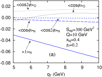
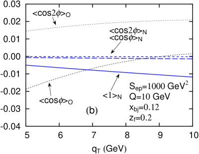
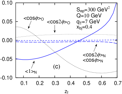
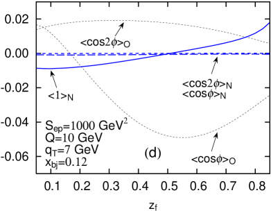
Figure 3: The azimuthal asymmetries for the $G_{F}$ contribution to $ep^{\uparrow}\to e\pi^{0}X$ at two energies. (a) and (b) show the $q_{T}$-dependence, while (c) and (d) show the $z_{f}$ dependence.

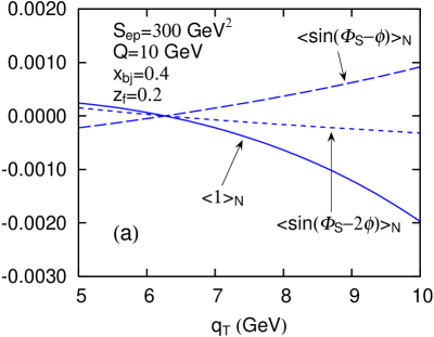
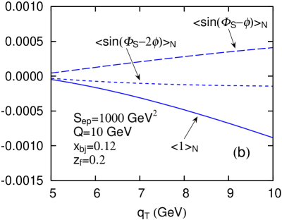
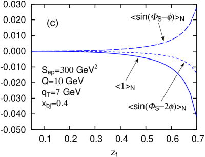
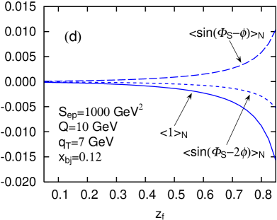
Figure 4: The azimuthal asymmetries for the $\widehat{E}_{F}$ contribution to $ep^{\uparrow}\to e\pi^{0}X$ at two energies. (a) and (b) show the $q_{T}$-dependence, while (c) and (d) show the $z_{f}$ dependence.

Appendix: Relation between twist-3 distributions

In the main text, we have discussed the relations (5)-(LABEL:gt) between the $D$-type and $F$-type twist-3 correlation functions for the transversely polarized nucleon. This appendix is devoted to demonstrate that $\widetilde{g}(x)$ of (LABEL:gt) can be expressed in terms of the $F$-type twist-3 correlation functions and the twist-2 quark helicity distibution $\Delta q(x)$ for the nucleon. Such relation involves the components with different number of partons, and can be obtained as a consequense of constraints from the equations of motion and Lorentz invariance.

We start with the well-known definition of the spin-dependent quark distributions of the nucleon [40, 30],

$$\int{d\lambda\over 2\pi}e^{i\lambda x}\langle pS|\bar{\psi}(0)[0,\lambda n]\gamma^{\mu}\gamma_{5}\psi(\lambda n)|pS\rangle=2M_{N}\left[\Delta q(x)p^{\mu}(S\cdot n)+g_{T}(x)S_{\perp}^{\mu}\right]+\cdots,$$ (38)

where $\Delta q(x)$ and $g_{T}(x)$ are the twist-2 and -3 quark distributions for the longitudinally and transversely polarized nucleon, respectively, and “$\cdots$” denotes Lorentz structure of twist higher than three. Using the QCD equations of motion, it can be shown [41] that $g_{T}(x)$ can be expressed in terms of the $D$-type functions as

$$g_{T}(x)=-\frac{1}{4x}\int dx^{\prime}\left[\widetilde{G}_{D}(x,x^{\prime})+\widetilde{G}_{D}(x^{\prime},x)+G_{D}(x,x^{\prime})-G_{D}(x^{\prime},x)\right].$$ (39)

Substituting the relations (5) and (6) into (39) and using the symmetrty properties (3), we get

$$g_{T}(x)=-\frac{1}{2x}\left(\widetilde{g}(x)+P\int_{-1}^{1}dx^{\prime}\frac{G_{F}(x,x^{\prime})+\widetilde{G}_{F}(x,x^{\prime})}{x-x^{\prime}}\right).$$ (40)

We note that this result has been obtained restricting the quark and gluon fields strictly on the lightcone. As is well-known, however, similar result can be obtained using the operator product expansion, where the fields are not restricted on the lightcone and thus the constraints from Lorentz invariance are fully taken into account. Here it is convenient to empoy the nonlocal version of the operator product expansion using the operator dentity [42, 30]

$$z_{\mu}\left(\frac{\partial}{\partial z_{\mu}}\bar{\psi}(0)\gamma^{\sigma}\gamma_{5}[0,z]\psi(z)-\frac{\partial}{\partial z_{\sigma}}\bar{\psi}(0)\gamma^{\mu}\gamma_{5}[0,z]\psi(z)\right)$$ (41)

$$= \int^{1}_{0}dt\bar{\psi}(0)[0,tz]\not{\!z}\left\{i\gamma_{5}\left(t-\frac{1}{2}\right)gF^{\sigma\rho}(tz)z_{\rho}-\frac{1}{2}g\tilde{F}^{\sigma\rho}(tz)z_{\rho}\right\}[tz,z]\psi(z)$$

$$+\,\left[\bar{\psi}(0)\gamma_{5}\sigma^{\sigma\rho}z_{\rho}[0,z]i\not{\!\!D}\psi(z)-\bar{\psi}(0)i\overleftarrow{\not{\!\!D}}\gamma_{5}\sigma^{\sigma\rho}z_{\rho}[0,z]\psi(z)\right],$$

where $z_{\mu}$ is not restricted on the lightcone. This identity is exact up to the irrelevant terms, i.e., the terms proportional to quark mass, the twist-4 ($O(z^{2})$) contributions, and the total derivatives. In the lightcone limit $z^{2}\rightarrow 0$, the nucleon matrix element of operators on both sides can be expressed in terms of the distribution functions defined in (38):

$$\langle p\ S|\bar{\psi}(0)[0,z]\gamma^{\mu}\gamma_{5}\psi(z)|p\ S\rangle = 2M_{N}\int_{-1}^{1}dxe^{-ixp\cdot z}\left(p^{\mu}\frac{S\cdot z}{p\cdot z}\left[\Delta q(x)-g_{T}(x)+O(z^{2})\right]\right.$$ (42)

$$+ \left.S^{\mu}\left[g_{T}(x)+O(z^{2})\right]\right)+\cdots,$$

and the $F$-type distributions of (2); note that the matrix element of the last line of (41) vanishes using the equations of motion. Thus the matrix element of (41) yields the differential equation

$$x\frac{dg_{T}(x)}{dx}+\Delta q(x)$$ (43)

$$=-\frac{1}{2}P\int_{-1}^{1}dx^{\prime}\frac{1}{x-x^{\prime}}\left\{\left(\frac{\partial}{\partial x}+\frac{\partial}{\partial x^{\prime}}\right)G_{F}(x,x^{\prime})+\left(\frac{\partial}{\partial x}-\frac{\partial}{\partial x^{\prime}}\right)\widetilde{G}_{F}(x,x^{\prime})\right\},$$

where we have used the symmetry relation (3). The solution of this equation with the boundary condition, $g_{T}(x)=0$ for $|x|>1$, reads

$$g_{T}(x) = \int^{\epsilon(x)}_{x}\frac{dx_{1}}{x_{1}}\left[\Delta q(x_{1})+\frac{1}{2}P\int_{-1}^{1}dx_{2}\frac{1}{x_{1}-x_{2}}\left\{\left(\frac{\partial}{\partial x_{1}}+\frac{\partial}{\partial x_{2}}\right)G_{F}(x_{1},x_{2})\right.\right.$$ (44)

$$\left.\left.+\left(\frac{\partial}{\partial x_{1}}-\frac{\partial}{\partial x_{2}}\right)\widetilde{G}_{F}(x_{1},x_{2})\right\}\right],$$

where $-1\leq x\leq 1$, and the first term on the RHS gives the Wandzura-Wilczek part for $g_{T}(x)$ [30]. It is straightforward to see that the moments $\int dxx^{n}g_{T}(x)$ using this solution reproduce the results obtained by the standard local operator expansion. Comparing (40) with (44), we find that $\widetilde{g}(x)$ is expressed in terms of $G_{F}(x_{1},x_{2})$, $\widetilde{G}_{F}(x_{1},x_{2})$, and $\Delta q(x)$, and get

$$\widetilde{g}(x)=-x\int^{\epsilon(x)}_{x}dx_{1}\left[\frac{2\Delta q(x_{1})}{x_{1}}+\frac{1}{x_{1}^{2}}P\int_{-1}^{1}dx_{2}\left\{\frac{G_{F}(x_{1},x_{2})}{x_{1}-x_{2}}+\left(3x_{1}-x_{2}\right)\frac{\widetilde{G}_{F}(x_{1},x_{2})}{(x_{1}-x_{2})^{2}}\right\}\right].$$ (45)

Combined with (6), this result shows that $\widetilde{G}_{D}(x_{1},x_{2})$ contains the contribution from the twist-2 operators corresponding to the Wandzura-Wilczek part, and the genuine twist-3 part of the $D$-type distributions $G_{D}(x_{1},x_{2})$, $\widetilde{G}_{D}(x_{1},x_{2})$ can be completely expressed in terms of the $F$-type distributions $G_{F}(x_{1},x_{2})$ and $\widetilde{G}_{F}(x_{1},x_{2})$.

References

-
[1]
G. Bunce et al., Phys. Rev. Lett. 36 (1976) 1113;
A. M. Smith et al., Phys. Lett. B185 (1987) 209;
B. Lundberg et al., Phys. Rev. D40 (1989) 3557;
E. J. Ramberg et al., Phys. Lett. B338 (1994) 403. - [2] D. L. Adams et al., Phys. Lett. B261 (1991) 201; ibid 264 (1991) 462.
-
[3]
M. Anselmino, A. Efremov and E. Leader, Phys. Rept. 261
(1995) 1 [Erratum-ibid. 281 (1997) 399];
Z. t. Liang and C. Boros, Int. J. Mod. Phys. A15 (2000) 927;
V. Barone, A. Drago and P. G. Ratcliffe, Phys. Rep. 359 (2002) 1. -
[4]
J. Adams et al. [STAR Collaboration],
Phys. Rev. Lett.
92 (2004) 171801;
D. A. Morozov, [STAR collaboration], hep-ex/0505024. - [5] S. S. Adler et al. [PHENIX Collaboration], Phys. Rev. Lett. 95 (2005) 202001.
- [6] F. Videbaek, [BRAHMS Collaboration], AIP Conf. Proc. 792 (2005) 993 [hep-ex/0508015].
-
[7]
A. Airapetian et al. [HERMES Collaboration],
Phys. Rev. Lett. 94 (2005) 012002;
M. Diefenthaler [HERMES Collaboration], AIP Conf. Proc. 792 (2005) 933 [hep-ex/0507013]. - [8] V. Y. Alexakhin et al. [COMPASS Collaboration], Phys. Rev. Lett. 94 (2005) 202002.
- [9] D. W. Sivers, Phys. Rev. D41 (1990) 83; Phys. Rev. D43 (1991) 261.
- [10] J. C. Collins, Nucl. Phys. B396 (1993) 161.
- [11] X. D. Ji, J. P. Ma and F. Yuan, Phys. Rev. D71 (2005) 034005; Phys. Lett. B597 (2004) 299.
- [12] J.C. Collins and D.E. Soper, Nucl. Phys. B193 (1981) 381; B213 (1983) 545(E).
- [13] J.C. Collins, D.E. Soper and G. Sterman, Nucl. Phys. B250 (1985) 199.
- [14] J. C. Collins, Phys. Lett. B536 (2002) 43.
- [15] A. V. Belitsky, X. D. Ji, and F. Yuan, Nucl. Phys. B656 (2003) 165.
- [16] D. Boer, P. Mulders and F. Pijlman, Nucl. Phys. B667 (2003) 201.
- [17] J. C. Collins and A. Metz, Phys. Rev. Lett. 93 (2004) 252001.
-
[18]
C. J. Bomhof, P. J. Mulders and F. Pijlman, Phys. Lett. B596 (2004) 277; hep-ph/0601171;
A. Bacchetta, C. J. Bomhof, P. J. Mulders and F. Pijlman, Phys. Rev. D72 (2005) 034030. - [19] For a review, see M. Anselmino et al., hep-ph/0511017.
- [20] A. V. Efremov and O. V. Teryaev, Sov. J. Nucl. Phys. 36 (1982) 140 [Yad. Phiz. 36 (1982) 242]; Phys. Lett. B150 (1985) 383.
- [21] J. Qiu and G. Sterman, Phys. Rev. Lett. 61 (1991) 381; Nucl. Phys. B378 (1992) 52.
- [22] J. Qiu and G. Sterman, Phys. Rev. D59 (1999) 014004.
- [23] Y. Kanazawa and Y. Koike, Phys. Lett. B1478 (2000) 121; Phys. Lett. B490 (2000) 99.
- [24] Y. Kanazawa and Y. Koike, Phys. Rev. D64 (2001) 034019.
- [25] Y. Koike, in “DIS2001” (Ed. by Baluni et al, World Scientific, 2002) 622. [hep-ph/0106260]
- [26] Y. Koike, AIP Conf. Proc. 675 (2003) 449 [hep-ph/0210396]; Nucl. Phys. A721 (2003) 364.
- [27] X. D. Ji, J. W. Qiu, W. Vogelsang and F. Yuan, hep-ph/0602239.
- [28] Y. Koike, in Proceedings of the RBRC workshop “Single Spin Asymmetries” (BNL, Upton, New York, June 1-3, 2005) Vol. 75 (BNL-74717-2005) 33.
- [29] X. Ji, Phys. Lett. B289 (1992) 137.
- [30] For a review of twist-3 distribution, see J. Kodaira and K. Tanaka, Prog. Theor. Phys. 101 (1999) 191.
- [31] X. D. Ji, Phys. Rev. D49 (1994) 114.
- [32] R. Meng, F. Olness and D. Soper, Nucl. Phys. B 371 (1992) 79.
-
[33]
Y. Koike and J. Nagashima, Nucl. Phys. B660 (2003) 269; B742 (2006) 312 (E);
Y. Koike, J. Nagashima and W. Vogelsang, Nucl. Phys. B744 (2006) 59. -
[34]
M. Luo, J. W. Qiu and G. Sterman, Phys. Rev. D50 (1994) 1951;
X. Guo, Phys. Rev. D58 (1998) 036001. - [35] A. Mendez, Nucl. Phys. B 145 (1978) 199.
- [36] M. Glück, E. Reya and A. Vogt, Eur. Phys. J. C 5 (1998) 461.
- [37] M. Glück, E. Reya, M. Stratmann and W. Vogelsang, Phys. Rev. D 63 (2001) 094005.
- [38] B. P. Kniehl, G. Kramer, B. Pötter, Nucl. Phys. B582 (2000) 514.
- [39] A. Deshpande, R. Milner, R. Venugopalan and W. Vogelsang, Ann. Rev. Nucl. Part. Sci. 55 (2005) 165 [arXiv:hep-ph/0506148].
- [40] R. L. Jaffe and X. D. Ji, Nucl. Phys. B 375 (1992) 527.
- [41] P. G. Ratcliffe, Nucl. Phys. B 264 (1986) 493.
- [42] I. I. Balitsky and V. M. Braun, Nucl. Phys. B 311 (1989) 541.
- [43] X. D. Ji, J. W. Qiu, W. Vogelsang and F. Yuan, hep-ph/0604128.