hep-ph/0604012

IFIC/06-08

Leptonic Charged Higgs Decays in the Zee Model
D. Aristizabal Sierra¹ and Diego Restrepo²

¹ AHEP Group, Instituto de Física Corpuscular – C.S.I.C./Universitat de València
Edificio de Institutos de Paterna, Apartado 22085, E–46071 València, Spain.

²Instituto de Física, Universidad de Antioquia
A.A. 1226  Medellín,  Colombia.

We consider the version of the Zee model where both Higgs doublets couple to leptons. Within this framework we study charged Higgs decays. We focus on a model with minimal number of parameters consistent with experimental neutrino data. Using constraints from neutrino physics we (i) discuss the reconstruction of the parameter space of the model using the leptonic decay patterns of both of the two charged Higgses, $h_{1,2}^{+}\rightarrow\ell_{j}^{+}\nu_{i}$, and the decay of the heavier charged Higgs, $h_{2}^{+}\rightarrow h^{+}_{1}h^{0}$; (ii) show that the decay rate $\Gamma(h_{1}^{+}\rightarrow\mu^{+}\nu_{i})$ in general is enhanced in comparision to the standard two Higgs doublet model while in some regions of parameter space $\Gamma(h_{1}^{+}\rightarrow\mu^{+}\nu_{i})$ even dominates over $\Gamma(h_{1}^{+}\rightarrow\tau^{+}\nu_{i})$.

1 Introduction

Neutrino oscillation experiments, including the results of KamLAND [1] have confirmed the LMA-MSW oscillation solution of the solar neutrino problem. Together with the earlier discoveries in atmospheric neutrinos [2], one can be fairly confident that all neutrino flavours mix and that at least two non-zero neutrino masses exist.

In the standard model neutrinos are massless. Among all the existing models to generate small neutrino Majorana masses the seesaw mechanism [3] is perhaps the most popular. However, this is not the only theoretical approach to neutrino masses. Other possibilities include Higgs triplets [4], supersymmetric models with broken $R$-parity [5, 6], some hybrid mechanisms that combine the triplet and the $R$-parity ideas [7] and radiative mechanisms [8, 9].

Here we consider a particular radiative mechanism, the Zee model [8]. In this model the scalar sector of the standard model is enlarged to include a charged SU(2) gauge singlet scalar and a second Higgs doublet. This particle content allows to write an explicit lepton number ($L$) violating term in the scalar potential and leads to neutrino masses at one loop order. In the Minimal Zee Model (MZM), only one Higgs doublet couples to leptons [10]. As a result, dangerous Flavour Changing Neutral Current (FCNC) processes are forbidden. It has been shown [11] that combining SNO, KamLAND and K2K experimental data this version is ruled out.

However, this does not mean that the Zee model is ruled out. The original version, from now on called the General Zee Model (GZM) [12], in which both of the two Higgs doublets couple to the matter fields has been shown [11, 12, 13] to be consistent with atmospheric and solar neutrino data as well [14].

Once one allows both of the Higgs doublets to couple to leptons the number of model parameters increases. Here instead of working with all the couplings of the model we will consider a scheme, previously discussed in references [12, 13], where the neutrino mass matrix has a two-zero-texture. This particular GZM will be called Next to MZM (NMZM).

In the Higgs sector, after spontaneous breaking of the electroweak symmetry, the charged gauge singlet mixes with the charged components of the two Higgs doublets. The resulting charged Higgs eigenstates ($h_{i}^{\pm}$ with $i=1,2$) decay to states with charged leptons and neutrinos. These decays can be used, in principle, to reconstruct the Majorana neutrino mass matrix.

We will show that due to the constraints imposed by neutrino physics, the $Br(h^{+}_{1}\to\sum_{i}\nu_{i}\mu^{+})$ is enhanced in comparision to the two-Higgs doublet models (2HDM) of type-I and type-II . Moreover, we will show that in large parts of the parameter space $Br(h^{+}_{1}\to\sum_{i}\nu_{i}\mu^{+})\gtrsim Br(h^{+}_{1}\to\sum_{i}\nu_{i}\tau^{+})$. For details see section 6.

The rest of this paper is organized as follows. In section 2 we give the generalities of the GZM and work out the Higgs mass spectrum of the model. In section 3 we study charged Higgs production at a future $e^{+}e^{-}$ collider. In section 4 we discuss the bounds on the parameters of the model coming from FCNC processes constraints. In section 5 we describe the Majorana neutrino mass matrix within the GZM and in the NMZM. In section 6 we discuss the connection between neutrino physics and charged Higgs decays. In section 7 we present our conclusions and summarize our results.

2 The Model

2.1 Generalities

If no new fermions are added to the standard model neutrino masses must be always of Majorana type, i.e. the mass term must violate $L$. In the Zee model an $L=2$ charged scalar, $h^{+}$, is introduced. Since this field carries electric charge its vacumm expectation value (vev) must vanish. Therefore in this model $L$ cannot be spontaneously broken. However, $h^{+}$ can be used to drive the lepton number breaking from the leptonic sector to the scalar sector. In order to accomplish this a new SU(2)_L doublet has to be added, as a result an explicit $L$ violation term can be written. This term is given by

$$\mu\epsilon_{\alpha\beta}H_{1}^{\alpha}H_{2}^{\beta}h^{-}+\mbox{H.c.}$$ (1)

where $\mu$ is a coupling with dimension of mass and $H_{1}$ and $H_{2}$ are doublets with hypercharge $Y_{1}=Y_{2}=1$.

The most general Yukawa couplings of the model can be written as

$$-{\cal L}_{Y}=\bar{L}_{i}(\Pi_{a})_{ij}H_{a}e_{Rj}+\epsilon_{\alpha\beta}\bar{L}^{\alpha}_{i}f_{ij}\,C(\bar{L}^{T})^{\beta}_{j}h^{-}+\text{H.c.}\,,$$ (2)

where $L_{i}$ are lepton doublets, $e_{Rj}$ are lepton singlets, $C$ is the charge conjugation operator, $\Pi_{a}$ ($a=1,2$) and $f$ are $3\times 3$ matrices in flavour space, $\epsilon_{\alpha\beta}$ ($\alpha,\beta=1,2$) is the SU(2)_L antisymmetric tensor and $i,j=1,2,3$ are family indices. $f$ is an antisymmetric matrix due to Fermi statistics.

In general both of the two Higgs doublets can acquire vev’s, $\langle H_{a}\rangle=v_{a}$, with $v=\sqrt{v_{1}^{2}+v_{2}^{2}}\simeq 246$ GeV. As usual, the ratio of these vev’s can be parametrized as $\tan\beta=v_{2}/v_{1}$.

2.2 Higgs potential and scalar mass spectrum

Though in this work we are interested mainly in the charged Higgs sector of the model and its relation with neutrino physics, we will briefly discuss the full scalar mass spectrum.

The Higgs potential is invariant under a global SO(2) transformation

$$\begin{pmatrix}H^{\prime}_{1}\\ H^{\prime}_{2}\end{pmatrix}=\begin{pmatrix}\cos\beta&\sin\beta\\ -\sin\beta&\cos\beta\end{pmatrix}\begin{pmatrix}H_{1}\\ H_{2}\end{pmatrix}.$$ (3)

Moreover, the Yukawa Lagrangian given in Eq. (2) is also invariant under the above transformation if the Yukawa matrices are appropriately rotated, namely

$$\begin{pmatrix}\Pi_{1}^{\prime}\\ \Pi_{2}^{\prime}\end{pmatrix}=\begin{pmatrix}\cos\beta&\sin\beta\\ -\sin\beta&\cos\beta\end{pmatrix}\begin{pmatrix}\Pi_{1}\\ \Pi_{2}\end{pmatrix}.$$ (4)

Therefore the full model is invariant under global SO(2) transformations of the two Higgs doublets. Thus, we are free to redefine our two doublet scalar fields by making an arbitrary SO(2) transformation. A particular choice of fields corresponds to a choice of basis. There is a basis in which only one of the two Higgs doublets acquire a vev. In the context of the 2HDM of type-III it is called the Higgs basis. Notice that in this basis $\tan\beta=0$.

In the Higgs basis the most general gauge invariant scalar potential of the model, consistent with renormalizability reads

$$V = \mu^{2}_{1}H_{1}^{\dagger}H_{1}+\mu^{2}_{2}H_{2}^{\dagger}H_{2}-[\mu^{2}_{3}H_{1}^{\dagger}H_{2}+\mbox{H.c.}]+\frac{1}{2}\lambda_{1}(H_{1}^{\dagger}H_{1})^{2}$$ (5)

$$+\frac{1}{2}\lambda_{2}(H_{2}^{\dagger}H_{2})^{2}+\lambda_{3}(H_{1}^{\dagger}H_{1})(H_{2}^{\dagger}H_{2})+\lambda_{4}(H_{1}^{\dagger}H_{2})(H_{2}^{\dagger}H_{1})$$

$$+\left\{\frac{1}{2}\lambda_{5}(H_{1}^{\dagger}H_{2})^{2}+[\lambda_{6}(H_{1}^{\dagger}H_{1})+\lambda_{7}(H_{2}^{\dagger}H_{2})]H_{1}^{\dagger}H_{2}+\mbox{H.c.}\right\}$$

$$+\mu_{h}^{2}|h^{+}|^{2}+\lambda_{h}|h^{+}|^{4}+\lambda_{8}|h^{+}|^{2}H_{1}^{\dagger}H_{1}+\lambda_{9}|h^{+}|^{2}H_{2}^{\dagger}H_{2}$$

$$+\lambda_{10}|h^{+}|^{2}(H_{1}^{\dagger}H_{2}+\mbox{H.c.})+\mu\epsilon_{\alpha\beta}H_{1}^{\alpha}H_{2}^{\beta}h^{-}.$$

Since we will not deal with CP-violating effects we only consider real coefficients

Minimization of the scalar potential, Eq. (5), leads to the conditions [16]

$$\mu_{1}^{2} = -\frac{1}{2}\lambda_{1}v^{2}$$

$$\mu_{3}^{2} = \frac{1}{2}\lambda_{6}v^{2}.$$ (6)

These conditions can be used to eliminate $\mu_{1}^{2}$ and $\mu_{3}^{2}$ as independent variables from $V$.

Of the original ten scalar degrees of freedom, three Goldstone bosons ($G^{\pm}$ and $G^{0}$) are absorbed by the $W^{\pm}$ and $Z^{0}$. The remaining seven physical Higgs particles are: two CP-even ($h^{0}$ and $H^{0}$ with $m_{h^{0}}\leq m_{H^{0}}$), one CP-odd ($A^{0}$) and two charged Higgs pairs ($h_{1}^{\pm}$ and $h_{2}^{\pm}$).

In the basis $\mathbf{\Phi}^{\dagger}=(G^{-},H^{-},h^{-})$ the squared-mass matrix for the charged Higgs states is given by

$${\cal M}_{C}^{2}=\begin{pmatrix}0&0&0\\ 0&M_{H^{\pm}}^{2}&-\mu v/\sqrt{2}\\ 0&-\mu v/\sqrt{2}&{\cal M}_{33}^{2}\end{pmatrix}\;,$$ (7)

where

$$M_{H^{\pm}}^{2} = \mu_{2}^{2}+\frac{1}{2}v^{2}\lambda_{3}$$

$${\cal M}_{33}^{2} = \mu_{h}^{2}+v^{2}\lambda_{8}.$$ (8)

The matrix element $M_{H^{\pm}}^{2}$ corresponds to the squared-mass of the charged scalars ($H^{\pm}$) that in the absence of the SU(2)_L singlets $h^{\pm}$ would be physical Higgs particles.

The squared-mass matrix ${\cal M}_{C}^{2}$ can be diagonalized by the rotation matrix

$$R=\begin{pmatrix}1&0&0\\ 0&\cos\varphi&\sin\varphi\\ 0&-\sin\varphi&\cos\varphi\end{pmatrix}\,.$$ (9)

where the angle $\varphi$ characterize the size of the $H^{\pm}-h^{\pm}$ mixing.

The mass eigenstate basis in the charged Higgs sector is defined as $\mathbf{H}^{\dagger}=(G^{-},h^{-}_{1},h^{-}_{2})$ and the rotation angle is given by

$$\sin 2\varphi=\frac{\sqrt{2}v\mu}{M_{2}^{2}-M_{1}^{2}}.$$ (10)

Here $M_{1}$ and $M_{2}$ stand for the masses of the scalars $h_{1}^{\pm}$ and $h_{2}^{\pm}$ which are given by

$$M_{1,2}^{2}=\frac{1}{2}\left(M_{H^{\pm}}^{2}+{\cal M}_{33}^{2}\mp\sqrt{(M_{H^{\pm}}^{2}-{\cal M}_{33}^{2})^{2}+2\mu^{2}v^{2}}\right).$$ (11)

In the Higgs basis the squared-masses for the CP-odd and CP-even Higgs states are given by [16]

$$M_{A^{0}}^{2} =M_{H^{\pm}}^{2}-\frac{1}{2}v^{2}(\lambda_{5}-\lambda_{4})$$

$$M_{H^{0},h^{0}}^{2} =\frac{1}{2}\left[M_{A^{0}}^{2}+v^{2}(\lambda_{1}+\lambda_{5})\pm\sqrt{[M_{A^{0}}^{2}+v^{2}(\lambda_{5}-\lambda_{1})]^{2}+4v^{4}\lambda_{6}^{2}}\right]$$ (12)

3 Charged Scalar Phenomenology

3.1 Cross section

In the following we discuss charged scalar $h^{\pm}_{k}$ ($k=1,2$) production at a future $e^{+}e^{-}$ collider. $h^{\pm}_{k}$ are produced in $e^{+}e^{-}$ annihilation via s-channel exchange of a $\gamma$ or $Z^{0}$ . The total cross section for the process $e^{+}e^{-}\to h_{k}^{+}h_{k}^{-}$ will be the sum of three terms

Figure 1: Production cross section for charged scalars $h_{k}^{\pm}$ at an 1 TeV $e^{+}e^{-}$ collider with unpolarized beams.

$$\sigma_{\mbox{\tiny{total}}}=\sigma_{\gamma}+\sigma_{Z}+\sigma_{\gamma Z}$$ (13)

corresponding to the pure photon, pure $Z$ and photon–$Z$ interference contributions respectively. Thus

$$\sigma_{\gamma} = \frac{1}{48\pi}\beta^{3}(g\,s_{w})^{4}\frac{1}{s}$$ (14)

$$\sigma_{Z} = \frac{1}{3072\pi}\beta^{3}\frac{g^{4}}{c^{4}_{w}}(W_{1k}^{2}-2s_{w}^{2})^{2}[(-1+4s_{w}^{2})^{2}+1]$$ (15)

$$\frac{s}{(s-M_{Z}^{2})^{2}+M_{Z}^{2}\Gamma_{Z}^{2}}$$

$$\sigma_{Z\gamma} = -\frac{1}{192\pi}\beta^{3}\frac{g^{4}s_{w}^{2}}{c_{w}^{2}}(W_{1k}^{2}-2s_{w}^{2})(-1+4s_{w}^{2})$$ (16)

$$\frac{s-M^{2}_{Z}}{(s-M_{Z}^{2})^{2}+M_{Z}^{2}\Gamma_{Z}^{2}}.$$

where $s_{w}=\sin\theta_{w}$, $c_{w}=\cos\theta_{w}$,

$$\beta=\sqrt{1-4\frac{M_{k}^{2}}{s}}$$ (17)

and $W_{11}=W_{22}=\cos\varphi$ and $W_{12}=-W_{21}=\sin\varphi$.

From Eqs. (2.2), (11) and (2.2) it can be noted that fixing $M_{1,2}$ does not fix $M_{H^{0},h^{0}}$ and $M_{A^{0}}$. Therefore, it is possible to take $M_{1,2}$ and $W_{1k}$ as free parameters without being in conflict with LEP bounds for the CP-even and CP-odd Higgs masses [17, 18, 19].

In Fig. 1 we show the cross section at an 1 TeV $e^{+}e^{-}$ collider with unpolarized beams. There we have taken $80\,\text{Gev}\leq M_{k}\leq 500\,\text{GeV}$. The spread in the plot is due to the dependence of the cross sections on $\varphi$. It is important to notice that for small (large) values of $\varphi$ the cross section for $h^{+}_{1}$ increases (decreases) while the cross section for $h^{+}_{2}$ decreases (increases). Figure 1 illustrates the situation for the case $\varphi=0$. In that case $h^{+}_{1}$ coincides with the SU(2) doublet $H^{+}$ (solid line) and $h^{+}_{2}$ with the SU(2) singlet $h^{+}$ (dashed line). The dotted-dashed line corresponds to $\cos\varphi\simeq 0.6$.

In Fig. 1 it can be seen that up to a mass of $\sim 350$ GeV the charged scalars have a cross section larger than 10 fb. Assuming an integrated luminosity of 1 ab^-1 this implies that at least 10⁴ charged scalar pairs will be produced.

3.2 Decay Widths

After the spontaneous electroweak symmetry breaking charged leptons acquire mass, namely

$$\widehat{M}_{\ell}=\frac{1}{\sqrt{2}}\sum_{a}v_{a}\Pi_{a}.$$ (18)

In the mass eigenstate basis for the charged scalars we have

$$-{\cal L}_{Y} \supset \bar{\nu}_{Li^{\prime}}O_{i^{\prime}j}e_{Rj}(\cos\varphi h^{+}_{1}-\sin\varphi h^{+}_{2})$$ (19)

$$+(\nu_{Li})^{T}C(2f_{ij})e_{Lj}(\sin\varphi h^{+}_{1}+\cos\varphi h^{+}_{2})+\text{H.c.}$$

where, in general, the couplings $O_{ij}$ are given by

$$O=-\sqrt{2}\frac{\tan\beta}{v}\widehat{M}_{\ell}+\frac{1}{\cos\beta}\Pi_{2}.$$ (20)

Charged scalars $h_{1,2}^{+}$ will decay through the couplings $O_{ij}$ and $f_{ij}$. Possible leptonic final states are $\nu_{i}\ell_{j}^{+}$. Possible final states involving quarks are $\bar{d}_{i}u_{j}$. These decays are determined by the couplings $O^{q}_{ij}$ where, in general

$$O^{q}=-\sqrt{2}\frac{\tan\beta}{v}\widehat{M}_{q}+\frac{1}{\cos\beta}\Pi_{2}^{q}.$$ (21)

Here $q$ refers to up-type and down-type quarks, $\widehat{M}_{q}$ are the diagonal quark mass matrices, and $\Pi_{2}^{q}$ are $3\times 3$ Yukawa coupling matrices of the second Higgs doublet. Notice that in the Higgs basis $\widehat{M}_{\ell}=(v/\sqrt{2})\Pi_{1}$ and $O=\Pi_{2}$.

We are interested in the widths and branching ratios for leptonic final states. The Lagrangian (19) determines the two body decays $h_{1,2}^{+}\to(\sum_{i}\nu_{i})\ell_{j}^{+}$. The decay rate reads

$$\Gamma(h_{k}^{+}\to(\sum_{i}\nu_{i})\ell_{j}^{+})=\frac{M_{k}}{16\pi}\sum_{i}[O_{ij}^{2}W_{1k}^{2}+(2f_{ij})^{2}W_{2k}^{2}]\,.$$ (22)

The couplings $h^{+}_{k}W^{-}Z$ and $h^{+}_{k}W^{-}\gamma$ do not exist in the Zee model. This can be understood as follows: since $h^{+}_{k}$ is a mixture of $H^{+}$ and $h^{+}$ these couplings are determined by the SU(2) doublet component. However, in the 2HDM of type-III these vertices do not exist [20]. Therefore the decays $h_{k}^{+}\rightarrow W^{+}\gamma$, $W^{+}Z^{0}$ in the Zee model are not present at tree level. For this reason we do not consider them.

Process	Constraint
$\mu^{-}\rightarrow e^{+}e^{-}e^{-}$	$|O_{12}O_{11}|<3.6\times 10^{-7}\left(\frac{M_{h}^{0}}{100\text{GeV}}\right)^{2}$
$\tau^{-}\rightarrow e^{+}e^{-}e^{-}$	$|O_{13}O_{11}|<1.3\times 10^{-3}\left(\frac{M_{h}^{0}}{100\text{GeV}}\right)^{2}$
$\tau^{-}\rightarrow\mu^{+}\mu^{-}\mu^{-}$	$|O_{13}O_{12}|<0.9\times 10^{-3}\left(\frac{M_{h}^{0}}{100\text{GeV}}\right)^{2}$
$\tau^{-}\rightarrow\mu^{-}\mu^{-}e^{+}$	$|O_{23}O_{21}|<0.9\times 10^{-3}\left(\frac{M_{h}^{0}}{100\text{GeV}}\right)^{2}$
$\tau^{-}\rightarrow e^{-}\mu^{-}e^{+}$	$|O_{13}O_{21}+O_{23}O_{11}|<1.0\times 10^{-3}\left(\frac{M_{h}^{0}}{100\text{GeV}}\right)^{2}$
$\tau^{-}\rightarrow e^{-}\mu^{-}\mu^{+}$	$|O_{13}O_{22}+O_{23}O_{12}|<1.0\times 10^{-3}\left(\frac{M_{h}^{0}}{100\text{GeV}}\right)^{2}$
$\mu^{-}\rightarrow e^{-}\gamma$	$|O_{12}O_{11}+O_{22}O_{21}+O_{32}O_{31}|<4.1\times 10^{-5}\left(\frac{M_{h}^{0}}{100\text{GeV}}\right)^{2}$
$\tau^{-}\rightarrow e^{-}\gamma$	$|O_{13}O_{11}+O_{23}O_{21}+O_{33}O_{31}|<4.7\times 10^{-2}\left(\frac{M_{h}^{0}}{100\text{GeV}}\right)^{2}$
$\tau^{-}\rightarrow\mu^{-}\gamma$	$|O_{13}O_{12}+O_{23}O_{22}+O_{33}O_{32}|<3.3\times 10^{-2}\left(\frac{M_{h}^{0}}{100\text{GeV}}\right)^{2}$

Table 1: Constraints on the parameters $O_{ij}$ from tree level and radiative FCNC processes induced by the neutral Higgs $h^{0}$.

4 Constraints from FCNC processes

In the GZM FCNC interactions are induced by the charged and neutral Higgses. Bounds on the $O_{ji}O_{km}$ couplings can be obtained from the non-observation of tree-level processes $\ell_{i}^{-}\rightarrow\ell_{j}^{+}\ell_{k}^{-}\ell_{m}^{-}$. Constraints on $O_{ki}O_{kj}$ come from radiative processes $\ell_{i}^{-}\rightarrow\ell_{j}^{-}\gamma$ induced by neutral Higgses. Limits on $f_{ik}f_{kj}$ and on $O_{ki}f_{kj}$ couplings come from radiative processes mediated by charged scalars. An important remark is that once the constraints on the $f_{ik}f_{kj}$ and $O_{ki}O_{kj}$ couplings are satisfied the limits on $O_{ki}f_{kj}$ are no longer important, for this reason we do not list them. Table 1 shows the constraints coming from the processes mediated by neutral scalars. Table 2 summarize the limits on the $f_{ij}$ parameters. Experimental constraints used in both tables were taken from [21]

5 Neutrino Physics

5.1 Neutrino Mass Matrix in the GZM

In this section we will discuss the neutrino mass matrix. The Majorana neutrino mass matrix in the Zee model arises at the one loop level through the exchange of the scalars $h^{\pm}_{1}$ and $h^{\pm}_{2}$ as shown in Fig. 2. Assuming $M_{1},M_{2}\gg m_{e},m_{\mu},m_{\tau}$ we have

$$(M_{\nu})_{ii^{\prime}}=\kappa[f_{ij}(\widehat{M}_{\ell})_{jj}O_{i^{\prime}j}+O_{ij}(\widehat{M}_{\ell})_{jj}f_{i^{\prime}j}]$$ (23)

where

$$\kappa=\frac{\sin 2\varphi}{(4\pi)^{2}}\ln\left(\frac{M^{2}_{2}}{M^{2}_{1}}\right).$$ (24)

Process	Constraint
$\mu^{-}\rightarrow e^{-}\gamma$	$|f_{23}f_{13}|<4.1\times 10^{-5}\left(\frac{M_{1}}{100\text{GeV}}\right)^{2}$
$\tau^{-}\rightarrow e^{-}\gamma$	$|f_{23}f_{12}|<4.7\times 10^{-2}\left(\frac{M_{1}}{100\text{GeV}}\right)^{2}$
$\tau^{-}\rightarrow\mu^{-}\gamma$	$|f_{13}f_{12}|<3.3\times 10^{-2}\left(\frac{M_{1}}{100\text{GeV}}\right)^{2}$

Table 2: Constraints on the parameters $f_{ij}$ coming from radiative FCNC processes induced by the charged Higgs $h_{1}^{\pm}$.

5.2 Neutrino Mass Matrix in the NMZM

In this section we discuss the neutrino mass matrix in the context of the NMZM. In our scheme the neutrino mass matrix is assumed to be

$$M_{\nu}=\kappa\begin{pmatrix}M_{ee}&M_{e\mu}&M_{e\tau}\\ M_{e\mu}&0&M_{\mu\tau}\\ M_{e\tau}&M_{\mu\tau}&0\end{pmatrix}.$$ (25)

The neutrino mass matrix, can be diagonalized by a matrix $U$, which can be parametrized as

$$U=\begin{pmatrix}1&0&0\\ 0&c_{23}&s_{23}\\ 0&-s_{23}&c_{23}\end{pmatrix}\times\begin{pmatrix}c_{13}&0&s_{13}\\ 0&1&0\\ -s_{13}&0&c_{13}\end{pmatrix}\times\begin{pmatrix}c_{12}&s_{12}&0\\ -s_{12}&c_{12}&0\\ 0&0&1\end{pmatrix},$$ (26)

where $s_{ij}=\sin\theta_{ij}$ and $c_{ij}=\cos\theta_{ij}$. Phases are zero since only real parameters are considered.

From

$$U^{T}M_{\nu}U=\widehat{M_{\nu}},$$ (27)

and taking the limit $\sin^{2}\theta_{13}=0$, since experimental neutrino data require $\sin^{2}\theta_{13}$ to be small [14], we can find approximate analytical expressions for the atmospheric and solar mixing angle as well as for $\Delta m_{23}^{2}$:

$$\tan^{2}\theta_{23} \simeq \left(\frac{M_{e\tau}}{M_{e\mu}}\right)^{2},$$

$$\tan 2\theta_{12} \simeq \sqrt{2}\frac{M_{e\mu}-M_{e\tau}}{M_{ee}+M_{\mu\tau}},$$ (28)

$$\sqrt{\Delta m_{23}^{2}} \simeq \frac{\kappa}{\sqrt{2}}(M_{e\mu}-M_{e\tau}).$$

Due to our two-zero-texture mass matrix (Eq. (25)) we have an inverted hierarchy neutrino mass spectrum [22] and therefore $M_{ee}\simeq M_{\mu\tau}$. Thus the neutrino mass matrix, Eq. (25), has only three independent entries which, from Eqs. (5.2), can be written in terms of $\tan^{2}\theta_{23}$, $\tan 2\theta_{12}$ and $\Delta m_{23}^{2}$, namely

$$M_{ee} \simeq M_{\mu\tau}\simeq\frac{\sqrt{\Delta m^{2}_{23}}}{\kappa\tan 2\theta_{12}}\,,$$

$$M_{e\mu} \simeq \frac{\sqrt{2\Delta m^{2}_{23}}}{\kappa(1+\tan\theta_{23})}\,,$$ (29)

$$M_{e\tau} \simeq -\frac{\tan\theta_{23}\sqrt{2\Delta m^{2}_{23}}}{\kappa(1+\tan\theta_{23})}\,.$$

Figure 2: Loop diagrams for Majorana neutrino mass. Here $i=1,2$

Assuming that there are no large hierarchies among the couplings $O_{i1}$ and $O_{ij}$, terms proportional to $m_{e}$, in the neutrino mass matrix, (see Eq. (23)) can be neglected. Thus we obtain Eq. (25) with $O_{23}=O_{32}=0$. Under this constraint the mass matrix depends on $\kappa$ and on the seven parameters

$$f_{12},f_{13},f_{23},O_{12},O_{13},O_{22},O_{33},$$ (30)

as can be seen from Eqs. (23) and (25). By using equations in (5.2) we can write four of these parameters in terms of the other three. Equations (56), (57), (58) and (59), in the appendix, give the expressions for $f_{12}$, $f_{13}$, $f_{23}$, $O_{13}$, in terms of $O_{12}$, $O_{22}$, and $O_{33}$. Note that both $f_{23}$ and $O_{33}$ must be different from zero.

Next we will consider the cases for which Eqs. (56), (57), (58) and (59) can be expressed in terms of a single parameter. We will call these cases the one-parameter solutions. Since $O_{33}$ cannot be zero (see Eq. (57)) we will parametrize all our one-parameter solutions in terms of this coupling. This leaves us with only four possibilities: $O_{12}=0$, $O_{13}=0$, $f_{12}=0$, $f_{13}=0$ and the remaining parameters in Eq. (30) different from zero in each case. We will show below that the first two lead to solutions with large $O_{33}$, while the last two lead to solutions with small $O_{33}$.

5.3 The one-parameter region

The main point here is that in these two cases (small and large $O_{33}$) not only neutrino physics but the decay patterns of $h^{\pm}_{1}$ are governed by a single parameter. This allows an analytical approach to the problem of identifying a particular collider signature that allows to distinguish between different regions in parameter space. In the following we will discuss the four possibilities mentioned previously and we will estimate the values of the parameters, consistent with neutrino physics as well as with FCNC constraints, in each case. This discussion will be useful in our analysis of the decays of $h_{1}^{+}$ presented in section 6.2.

5.3.1 The large $O_{33}$ case

Choosing $O_{12}=0$ and $O_{22}=(m_{\mu}/m_{\tau})O_{33}$, as in references [12, 13], Eqs. (56), (57), (58) and (59) are reduced to the one-parameter solution

$$f_{12}\approx \frac{\left[1+\left(2+4\,\tan^{2}2\theta_{12}\right)\,\tan\theta_{23}+\tan^{2}\theta_{23}\right]\,}{2\,\sqrt{2}\,\kappa\,\tan^{2}2\theta_{12}\,\tan\theta_{23}\,\left(1+\tan\theta_{23}\right)}\frac{\sqrt{\Delta m_{23}^{2}}\,m_{\tau}}{m_{\mu}^{2}}\frac{1}{O_{33}}\sim\frac{6.3\times 10^{-9}}{\kappa\,O_{33}},$$

$$f_{13}\approx -\frac{\sqrt{2}\,\tan\theta_{23}}{\kappa\,\left(1+\tan\theta_{23}\right)}\frac{\sqrt{\Delta m_{23}^{2}}}{m_{\tau}}\frac{1}{O_{33}\,}\sim-\frac{1.9\times 10^{-11}}{\kappa\,O_{33}},$$ (31)

$$f_{23}\approx \frac{1}{\kappa\,\tan 2\theta_{12}}\frac{\sqrt{\Delta m_{23}^{2}}}{m_{\tau}}\frac{1}{O_{33}\,}\sim\frac{1.2\times 10^{-11}}{\kappa\,O_{33}},$$

$$O_{13}\approx -\frac{1+\tan\theta_{23}}{2\,\sqrt{2}\,\tan 2\theta_{12}\,\tan\theta_{23}}O_{33}\sim-0.3\,O_{33}.$$

The last values in each equation are obtained using the best fit point value for each neutrino observable.

An upper bound for $\kappa$ can be estimated using the fact that

$$\kappa=\frac{\sin 2\varphi}{(4\pi)^{2}}\ln\left(\frac{M^{2}_{2}}{M^{2}_{1}}\right)=\frac{\sqrt{2}v\mu}{(4\pi)^{2}}\frac{1}{M_{2}^{2}-M_{1}^{2}}\ln\left(\frac{M^{2}_{2}}{M^{2}_{1}}\right)\simeq\frac{\sqrt{2}}{(4\pi)^{2}}\frac{v\mu}{M_{2}^{2}}.$$ (32)

Therefore for $M_{2}<1000\,$GeV and $|\mu|<500\,$GeV [23], we have that $|\kappa|\lesssim 10^{-2}$. For example for $M_{1}=200\,$GeV, $M_{2}=300\,$GeV, and $\mu=100\,$GeV, we have

$$\sin 2\varphi=0.7\qquad\text{and}\qquad\kappa=3.6\times 10^{-3}.$$ (33)

On the other hand, from the expression for $f_{12}$ in Eq. (31) and imposing $f_{12}\lesssim 10^{-2}$ a lower bound on $\kappa$ can be found. Choosing $O_{33}\lesssim 10^{-2}$, we have that $|\kappa|\gtrsim 10^{-5}$. For example, for $\mu=2\,$GeV and with $M_{1}$ and $M_{2}$ as in the previous case, we have

$$\sin 2\varphi=0.014\qquad\text{and}\qquad\kappa=7.2\times 10^{-5}.$$ (34)

Using the value of $\kappa$ given in Eq. (33) we have

$$f_{12}\sim\frac{1.8\times 10^{-6}}{O_{33}},\qquad f_{13}\sim-\frac{5.2\times 10^{-9}}{O_{33}},\qquad f_{23}\sim\frac{3.2\times 10^{-9}}{O_{33}}.\qquad$$ (35)

Now instead of $O_{12}=0$ we choose $O_{13}=0$. Again, as in the previous case, we take $O_{22}=(m_{\mu}/m_{\tau})O_{33}$ and the best fit point values for each neutrino observable. With $\kappa$ given by (33), Eqs. (56), (57), (58) and (59) become

$$f_{12}\sim\frac{1.5\times 10^{-6}}{O_{33}},\;f_{13}\sim-\frac{5.2\times 10^{-9}}{O_{33}},\;f_{23}\sim\frac{3.2\times 10^{-9}}{O_{33}},\;O_{13}\sim 0.02\,O_{33},$$ (36)

which is basically the same result obtained in the case with $O_{12}=0$ (Eqs. (35)).

From Eqs. (35) and (36) it can be seen that all the parameters can be below $10^{-3}$, with a hierarchy of order $10^{3}$ between $f_{12}$ and the others $f_{ij}$. In this way the constraints on the couplings coming from FCNC interactions (Tables 1 and 2) are always satisfied.

Note that $f_{12}\lesssim 10^{-2}$ requires $O_{33}\gtrsim 10^{-4}$. Therefore the range of variation of $O_{33}$ is restricted to $10^{-4}\lesssim O_{33}\lesssim 10^{-2}$. For $\kappa$ small, as in Eq. (34), $O_{33}\sim 10^{-2}$.

5.3.2 The small $O_{33}$ case

If we choose $f_{13}=0$ and, in order to define the one-parameter solution in this case $O_{22}=0$, Eqs. (56), (57), (58) and (59) become

$$f_{12}\approx \frac{\left(1+\tan\theta_{23}\right)}{2\,\sqrt{2}\,\kappa\,\tan 2\theta_{12}^{2}\,\tan\theta_{23}}\frac{\sqrt{\Delta m_{23}^{2}}}{m_{\tau}\,}\frac{1}{O_{33}}\sim\frac{3.6\times 10^{-12}}{\kappa\,O_{33}},$$

$$f_{23}\approx \frac{1}{\kappa\,\tan 2\theta_{12}}\frac{\sqrt{\Delta m_{23}^{2}}}{m_{\tau}}\frac{1}{O_{33}}\sim\frac{1.2\times 10^{-11}}{\kappa\,O_{33}},$$ (37)

$$O_{12}\approx \frac{{\sqrt{2}}\,\tan 2\theta_{12}\,\tan\theta_{23}}{\left(1+\tan\theta_{23}\right)}\frac{m_{\tau}}{m_{\mu}}O_{33}\sim 27\,O_{33},$$

$$O_{13}\approx \frac{\sqrt{2}\,\tan 2\theta_{12}}{1+\tan\theta_{23}}O_{33}\sim 1.6\,O_{33}.$$

The last values in each equation are obtained using the best fit point values for each neutrino observable. Note that $O_{12}\lesssim 10^{-2}$ requires $O_{33}\lesssim 4\times 10^{-4}$.

On the other hand, from the expression for $f_{23}$ in Eq. (37), if $O_{33}\lesssim 4\times 10^{-4}$ and we impose the bound $f_{23}\lesssim 10^{-2}$ we have that $\kappa\gtrsim 3\times 10^{-6}$. For example, if we choose $\mu=0.2\,$GeV, $M_{1}=200$ GeV and $M_{2}=300$ GeV , we have

$$\sin 2\varphi=1.4\times 10^{-3}\qquad\text{and}\qquad\kappa=7.2\times 10^{-6}$$ (38)

For the value of $\kappa$ given in Eq. (33), that satisfies the bound $\kappa\gtrsim 3\times 10^{-6}$, with $M_{1}=200\,$ GeV and $M_{2}=300\,$GeV we have

$$f_{12}\sim\frac{1\times 10^{-9}}{O_{33}},\quad f_{23}\sim\frac{3.2\times 10^{-9}}{O_{33}}.$$ (39)

Now instead of $f_{13}=0$ we choose $f_{12}=0$. Using the best fit point values for each neutrino observable, $O_{22}=0$ and $\kappa$ given by Eq. (33), Eqs. (56), (57), (58) and (59) become

$$f_{13}\sim\frac{9.8\times 10^{-10}}{O_{33}},\;f_{23}\sim\frac{3.2\times 10^{-9}}{O_{33}},\;O_{12}\sim 32\,O_{33},\;O_{13}\sim 1.6\,O_{33}.$$ (40)

In both cases ($f_{12}=0$ or $f_{13}=0$) we can have all the five parameters of order of $10^{-4}$ without any hierarchy among them. In fact, the case $f_{12}=0$, considered here, is a particular case of the one studied in reference [11] in which all the parameters $O_{ij}$ and $f_{ij}$ are of the same order of magnitude. From Tables 1 and 2 it can be seen that FCNC constraints are always satisfied.

Case	$O_{33}$	$\kappa$	$\mu$ (GeV)
Large $O_{33}$	$10^{-4}$ – $10^{-2}$	$10^{-5}$ – $10^{-2}$	2 – 500
Small $O_{33}$	$10^{-7}$ – $4\times 10^{-3}$	$3\times 10^{-6}$ – $10^{-2}$	$0.2$ – 500

Table 3: Range of $O_{33}$, $\kappa$ and $\mu$ for the one-parameter solutions in the NMZM

A lower bound on $O_{33}$ can be obtained using the bound $f_{23}\lesssim 10^{-2}$. Together with the upper bound estimated previously we have $10^{-7}\lesssim O_{33}\lesssim 4\times 10^{-3}$. Notice that for smaller values of $\kappa$, as the one in Eq. (38), the range of variation is more restricted, $10^{-5}\lesssim O_{33}\lesssim 4\times 10^{-3}$.

It is worth noticing that there are no more possibilities in the one-parameter solution case. The large $O_{33}$ case, obtained when either $O_{12}$ or $O_{13}$ are neglected implies a hierarchy among the non zero $f_{ij}$ and, depending on the case, on $O_{12}$ or $O_{13}$. In the small $O_{33}$ case, obtained when either $f_{12}$ or $f_{13}$ are neglected, it is possible to have all the parameters at the level of $10^{-4}$. Table 3 shows the allowed range of variation for $O_{33}$, $\kappa$ and $\mu$ in each case.

6 Neutrino and Collider Physics

6.1 Determination of the Neutrino Mass Matrix Parameters

In this section we discuss how the charged scalar decays can give some hints about the parameters that determine neutrino masses and mixing angles. Charged Higgs decays are governed by the same parameters that control neutrino physics so, in principle, the information coming from these decays can be used to reconstruct the neutrino mass matrix. Outside of the one-parameter regions analysed in section 5 the number of parameters is large and since neutrino flavour cannot be determined the mass matrix cannot be, in general, reconstructed. Despite this, in the limiting case of small mixing ($\varphi\ll 1$), the fact that the the mainly doublet state decays are dictated by the $O_{ij}$ and the mainly singlet state decays are controlled by the $f_{ij}$ leads to a situation in which the reconstruction of part of the parameter space of the model is possible.

The charged scalar singlet $h^{+}$ does not couples to quarks. Thus experimentally the mainly singlet state can be differentiated from the mainly doublet state by the fact that the branching ratio to final states with quarks ($\bar{u}_{i}d_{j}$) must be smaller for the former than for the latter. Our main assumption here is that all the decays that we are going to consider have a branching ratio in the order of at least per-mille.

In the following discussion we will use the notation $h^{+}_{d,s}$ for charged Higgses. Here $d$ and $s$ denote the mainly doublet and mainly singlet states respectively. Note that $d=1\;,s=2$ or $d=2\;,s=1$ are possible. Ratios of branching ratios for $h_{d,s}^{+}$ can be used to obtain information about the $O_{ij}$ and $f_{ij}$ couplings. In the case of $h_{d}^{+}$ we have

$$\frac{Br(h_{d}^{+}\to(\sum_{i}\nu_{i})\ell^{+}_{j})}{Br(h_{d}^{+}\to(\sum_{k}\nu_{k})\ell^{+}_{s})}\simeq\frac{\sum_{i}O_{ij}^{2}}{\sum_{k}O_{ks}^{2}}$$ (41)

and for $h_{s}^{+}$

$$\frac{Br(h_{s}^{+}\to(\sum_{i}\nu_{i})\ell^{+}_{j})}{Br(h_{s}^{+}\to(\sum_{k}\nu_{k})\ell^{+}_{s})}\simeq\frac{\sum_{i}f_{ij}^{2}}{\sum_{k}f_{ks}^{2}}.$$ (42)

Corrections to both ratios are $\propto\varphi^{2}\lll 1$. The interesting point here is that despite the large number of parameters the relative size of the $f_{ij}$ couplings can be obtained by suitable combinations of ratios of branching ratios, for example

$$\frac{Br^{\mu}_{s}-Br^{\tau}_{s}+Br^{e}_{s}}{Br^{\mu}_{s}-Br^{e}_{s}+Br^{\tau}_{s}}\simeq\frac{f_{12}^{2}}{f_{23}^{2}}$$ (43)

with $Br^{\ell_{j}}_{s}$ denoting $Br(h_{s}^{+}\to(\sum_{i}\nu_{i})\ell^{+}_{j})$. For the $O_{ij}$ the situation is more complicated but even in this case some information can be obtained from the ratios of branching ratios. For example, the relation

$$\frac{Br(h_{d}^{+}\to(\sum_{i}\nu_{i})\mu^{+})}{Br(h_{d}^{+}\to(\sum_{k}\nu_{k})e^{+})}\simeq\frac{O_{12}^{2}+O_{22}^{2}}{O_{11}^{2}+O_{21}^{2}+O_{31}^{2}}$$ (44)

allows to determine the relative importance of the couplings involved in these decays.

Figure 3: Ratio of branching ratios $Br^{\mu\tau e}_{s}/Br^{\mu e\tau}_{s}=(Br^{\mu}_{s}-Br^{\tau}_{s}+Br^{e}_{s})/(Br^{\mu}_{s}-Br^{e}_{s}+Br^{\tau}_{s})$ versus $f_{12}^{2}/f_{23}^{2}$ (left) and $Br^{\mu}_{d}/Br^{e}_{d}=Br(h_{d}^{+}\to(\sum_{i}\nu_{i})\mu^{+})/Br(h_{d}^{+}\to(\sum_{k}\nu_{k})e^{+})$ versus $O_{\mu}^{2}/O_{e}^{2}=(O_{12}^{2}+O_{22}^{2})/(O_{11}^{2}+O_{21}^{2}+O_{31}^{2})$ (right). See text.

Figure 3 shows the ratios of branching ratios described above. Any deviation from the small mixing assumption would lead to a large dispersion.

Figure 4: Ratio of branching ratios indicated by the variables $y_{1}$ (left) and $y_{2}$ (right) versus the atmospheric and solar mixing angles indicated by the variables $x_{1}$ (left) and $x_{2}$ (right). See text

There are two limit cases of particular interest where the decays of $h_{d,s}^{+}$ are correlated with the neutrino mixing angles, $O_{12}\ll O_{13}\ll O_{22}<O_{33}$ or $O_{13}\ll O_{12}\ll O_{22}<O_{33}$. Figure 4 shows both cases. In the left plot the variables $y_{1}$ and $x_{1}$ are given by

$$y_{1} =\sqrt{\frac{Br^{\mu}_{s}-Br^{e}_{s}+Br^{\tau}_{s}}{Br^{e}_{s}-Br^{\mu}_{s}+Br^{\tau}_{s}}}\left(1-\frac{m_{\mu}}{m_{\tau}}\sqrt{\frac{Br(h_{d}^{+}\to(\sum_{i}\nu_{i})\mu^{+})}{Br(h_{d}^{+}\to(\sum_{k}\nu_{k})\tau^{+})}}\right)$$

$$x_{1} =\frac{1}{\sqrt{2}\tan 2\theta_{12}}\left(1+\frac{1}{\tan\theta_{23}}\right).$$ (45)

In the right one the variables $y_{2}$ and $x_{2}$ are defined as

$$y_{2} =\sqrt{\frac{Br^{\mu}_{s}-Br^{e}_{s}+Br^{\tau}_{s}}{Br^{\mu}_{s}-Br^{\tau}_{s}+Br^{e}_{s}}}\left(\frac{m_{\tau}}{m_{\mu}}\sqrt{\frac{Br(h_{d}^{+}\to(\sum_{i}\nu_{i})\tau^{+})}{Br(h_{d}^{+}\to(\sum_{k}\nu_{k})\mu^{+})}}-1\right)$$

$$x_{2} =\frac{1}{\sqrt{2}\tan 2\theta_{12}}\left(1+\tan\theta_{23}\right)$$ (46)

Figure 5: Decay rate $\Gamma(h_{2}^{+}\rightarrow h^{+}_{1}h^{0})$ versus $\mu^{2}$ for fixed values $M_{2}=400\,\text{Gev}$, $M_{1}=150\,\text{Gev}$ and $M_{h^{0}}=130\,\text{GeV}$.

Another important decay, if kinematically allowed, that could be used to obtain information about $\mu$ is $h_{2}^{+}\rightarrow h^{+}_{1}h^{0}$. The decay rate for this process reads

$$\Gamma(h_{2}^{+}\rightarrow h^{+}_{1}h^{0})=\frac{1}{16\pi}\frac{\Lambda^{2}}{M_{2}}\sqrt{1-4\frac{M_{1}^{2}}{M_{2}^{2}}}.$$ (47)

Here

$$\Lambda=\frac{\mu}{\sqrt{2}}\sin\alpha\cos 2\varphi+v\frac{\sin 2\varphi}{2}(\Lambda_{22}-\Lambda_{33})$$ (48)

and

$$\Lambda_{22} =\lambda_{7}\cos\alpha-\lambda_{3}\sin\alpha,$$

$$\Lambda_{33} =\lambda_{10}\cos\alpha-\lambda_{8}\sin\alpha$$ (49)

where $\alpha$ is the mixing angle that define the two CP-even Higgs mass eigenstates, $h^{0}$ and $H^{0}$.

Figure 5 shows the decay rate $\Gamma(h_{2}^{+}\rightarrow h^{+}_{1}h^{0})$ versus $\mu^{2}$. There we have fixed $M_{2}=400\,\text{Gev}$, $M_{1}=150\,\text{Gev}$, $M_{h^{0}}=130\,\text{GeV}$ and $\alpha=\pi/6$. $\mu$ is in the range $0.1\,\text{GeV}-8\,\text{Gev}$ in order to ensure $\varphi\ll 1$. The dispersion is due to the presence of the other couplings, present in the scalar potential (Eq. (5)). Apart from allowing the approximate determination of $\mu$, measurements of $\Gamma(h_{2}^{+}\rightarrow h^{+}_{1}h^{0})$ in the range indicated by Fig. 5 will indicate that the small mixing limit is realized.

6.2 Hierarchy of charged Higgs leptonic decays

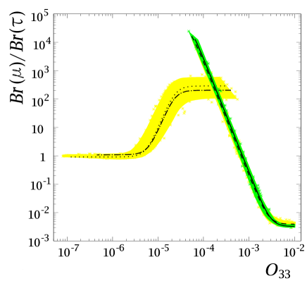
Figure 6: ${Br(h_{1}^{+}\to(\sum_{i}\nu_{i})\mu^{+})}/{Br(h_{1}^{+}\to(\sum_{i}\nu_{i})\tau^{+})}$ as a function of $O_{33}$ for $3\times 10^{-6}<\kappa<10^{-2}$ obtained with $0.2<\mu<500\,$GeV, $M_{1}=200\,$GeV and $M_{2}=500\,$GeV. All the parameters $f_{ij}$ and $O_{ij}$ satisfy the bounds shown in Tables 1 and 2. For all the dark gray (green) points $O_{12}<10^{-6}$. See text

In this section we will show that in the NMZM, the decay process $h_{1}^{+}\to(\sum_{i}\nu_{i})\mu^{+}$ is enhanced in comparision to the 2HDM of type-I and type-II. Moreover, it is shown that in large parts of the parameter space, $h_{1}^{+}\to(\sum_{i}\nu_{i})\mu^{+}$ can be the dominant leptonic decay.

In the one-parameter solutions, described in sec. 5, the parameters $O_{12}$, $O_{13}$, $f_{12}$, $f_{13}$ and $f_{23}$ are governed by the parameter $O_{33}$. In this way the $Br(h^{+}_{1}\rightarrow(\sum_{i}\nu_{i})\ell_{j}^{+})$ are functions of $O_{33}$. In order to find expressions with no dependence on $\kappa$ or $O_{33}$ and correlated with neutrino physics observables ($\tan 2\theta_{12}$, $\tan\theta_{23}$) we consider ratios of branching ratios in the limits $O_{ij}\gg f_{ij}$ and $O_{ij}\ll f_{ij}$, namely

$$\frac{Br(h_{1}^{+}\to(\sum_{i}\nu_{i})\mu^{+})}{Br(h_{1}^{+}\to(\sum_{i}\nu_{i})\tau^{+})}= \frac{\sum_{i}[(O_{i2}\cos\varphi)^{2}+(2f_{i2}\sin\varphi)^{2}]}{\sum_{i}[(O_{i3}\cos\varphi)^{2}+(2f_{i3}\sin\varphi)^{2}]}$$ (50)

$$\approx \begin{cases}\displaystyle{\frac{\sum_{i}O_{i2}^{2}}{\sum_{i}O_{i3}^{2}}}&\text{for $O_{ij}\gg f_{ij}$}\\ \displaystyle{\frac{\sum_{i}f_{i2}^{2}}{\sum_{i}f_{i3}^{2}}}&\text{for $O_{ij}\ll f_{ij}$}\end{cases}$$ (51)

Clearly from Eqs. (31) or (37), Eq. (51) depend only on the neutrino mixing angles and charged lepton masses. We will call the regions of parameter space with either $O_{ij}$ or $f_{ij}$ dominance correlation regions. Ratio of branching ratios in these regions are $\kappa$ independent (or $\mu$ independent). In general, outside the correlation regions, the independence on $\mu$ approximately holds, but there is a dependence on $M_{2}$.

Fig. 6 shows the ratio ${Br(h_{1}^{+}\to(\sum_{i}\nu_{i})\mu^{+})}/{Br(h_{1}^{+}\to(\sum_{i}\nu_{i})\tau^{+})}$ as function of $O_{33}$. For all curves, we have used the best fit point values for $\Delta m_{23}^{2}$, and the solar and atmospheric mixing angles. We have taken also $3\times 10^{-6}<\kappa<10^{-2}$ obtained when $0.2<\mu<500\,$GeV, $M_{1}=200\,$GeV and $M_{2}=500\,$GeV. The correlation regions correspond to the flat parts of the curves. The large $O_{33}$ case determined by Eq. (31) with $O_{12}=0$ corresponds to the solid line in the right part of the plot, while the large $O_{33}$ case with $O_{13}=0$ correspond to the dashed line. In the same way, the small $O_{33}$ case described by Eq. (37) with $f_{13}=0$ corresponds to the dotted line in the left part of the plot, while the small $O_{33}$ case with $f_{12}=0$ correspond to the dotted–dashed line. The scatter plot was obtained by searching for all solutions compatible with neutrino data at 3$\sigma$ level, and keeping $O_{22}=(m_{\mu}/m_{\tau})\,O_{33}$.

In the large $O_{33}$ case described by Eq. (31), the correlation region for $f_{ij}\gg O_{ij}$ is excluded because the parameters $f_{ij}$ are above the values consistent with FCNC constraints (see Tables 1 and 2). For the other correlation region, for which $O_{ij}\gg f_{ij}$, we have

$$\frac{Br(h_{1}^{+}\to(\sum_{i}\nu_{i})\mu^{+})}{Br(h_{1}^{+}\to(\sum_{i}\nu_{i})\tau^{+})}\sim\left(\frac{m_{\mu}}{m_{\tau}}\right)^{2}\qquad\text{for $O_{ij}\gg f_{ij}$}.$$ (52)

As shown by the solid line at the right of Fig. 6, the contribution of $f_{ij}$ can increase the ratio of branchings ratios up to a factor of $10^{7}$. In this way the decay $h_{1}^{+}\rightarrow(\sum_{i}\nu_{i})\mu^{+}$ may become observable in future colliders. The dark gray (green) points were selected from the full scatter plot by choosing $O_{12}<10^{-6}$. They are well fitted by the solid line which represents the one-parameter solution with $O_{12}=0$ as given in Eq. (31).

In the small $O_{33}$ case with $f_{13}=0$, we have

$$\frac{Br(h_{1}^{+}\to(\sum_{i}\nu_{i})\mu^{+})}{Br(h_{1}^{+}\to(\sum_{i}\nu_{i})\tau^{+})}$$

$$\approx\begin{cases}\displaystyle{\frac{2\,\tan^{2}2\theta_{12}\,\tan^{2}\theta_{23}}{2\,\tan^{2}2\theta_{12}+{\left(1+\tan\theta_{23}\right)}^{2}}\frac{m_{\tau}^{2}}{m_{\mu}^{2}\,}}&\text{for $O_{ij}\gg f_{ij}$}\\ \displaystyle{\frac{1+2\,\tan\theta_{23}+\left(1+8\,\tan^{2}2\theta_{12}\right)\,\tan^{2}\theta_{23}}{8\,\tan^{2}2\theta_{12}\,\tan^{2}\theta_{23}}}&\text{for $O_{ij}\ll f_{ij}$}\end{cases}$$

$$\sim\begin{cases}\displaystyle{\tan^{2}\theta_{23}\left(\frac{m_{\tau}}{m_{\mu}}\right)^{2}}&\text{for $O_{ij}\gg f_{ij}$}\\ 1&\text{for $O_{ij}\ll f_{ij}$.}\end{cases}$$ (53)

As shown in the left part of Fig. 6, in this case the ratio of branching ratios is larger than one, and therefore an inverted hierarchy for the leptonic decays of the lightest charged Higgs is obtained. In this way, in the small $O_{33}$ case, the most important leptonic decay channel for the charged Higgs $h^{+}_{1}$ must be $h^{+}_{1}\rightarrow(\sum_{i}\nu_{i})\mu^{+}$ instead of $h^{+}_{1}\rightarrow(\sum_{i}\nu_{i})\tau^{+}$.

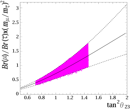
Figure 7: ${Br(h_{1}^{+}\to(\sum_{i}\nu_{i})\mu^{+})}/{Br(h_{1}^{+}\to(\sum_{i}\nu_{i})\tau^{+})}(m_{\mu}/m_{\tau})^{2}$ as a function of $\tan\theta_{23}$ in the correlation region $O_{ij}\gg f_{ij}$ of the small $O_{33}$ case. The solid curve corresponds to the best fit point value of $\tan 2\theta_{12}$, while the upper and lower curves corresponds to its $3\sigma$ limits. See text.

Fig. 7 shows the correlation region for $O_{ij}\gg f_{ij}$ in the small $O_{33}$ case. The curves correspond to the ratio ${Br(h_{1}^{+}\to(\sum_{i}\nu_{i})\mu^{+})}/{Br(h_{1}^{+}\to(\sum_{i}\nu_{i})\tau^{+})}$, normalized by $(m_{\mu}/m_{\tau})^{2}$, as a function of the atmospheric mixing angle, as expected from Eq. (6.2) for the best fit point value of $\tan 2\theta_{12}$ (solid line) and its 3$\sigma$ limits (dashed lines). The parameters are fixed as in Fig. 6 and the spread of the points can be understood from the uncertainty in the solar mixing angle. In this region the charged Higss decay rate $\Gamma(h^{+}\rightarrow(\sum_{i}\nu_{i})\mu^{+})$ can be larger than decay rate $\Gamma(h^{+}\rightarrow(\sum_{i}\nu_{i})\tau^{+})$ up to a factor of $(m_{\tau}/m_{\mu})^{2}=280$.

From Fig. 6 it can be seen that the large $O_{33}$ region is divided in three sub-regions, region I where $10^{-3}\lesssim Br(h_{1}^{+}\to(\sum_{i}\nu_{i})\mu^{+})/Br(h_{1}^{+}\to(\sum_{i}\nu_{i})\tau^{+})\lesssim 1$, region II for which $1\lesssim Br(h_{1}^{+}\to(\sum_{i}\nu_{i})\mu^{+})/Br(h_{1}^{+}\to(\sum_{i}\nu_{i})\tau^{+})\lesssim 10^{2}$ and region III characterised by $10^{2}\lesssim Br(h_{1}^{+}\to(\sum_{i}\nu_{i})\mu^{+})/Br(h_{1}^{+}\to(\sum_{i}\nu_{i})\tau^{+})\lesssim 10^{4}$. Measurements of the ratio $Br(h_{1}^{+}\to(\sum_{i}\nu_{i})\mu^{+})/Br(h_{1}^{+}\to(\sum_{i}\nu_{i})\tau^{+})$ are sufficient to decide whether region I or III are realized. In region III there is an ambiguity that cannot be removed by measurements of the ratio $Br(h_{1}^{+}\to(\sum_{i}\nu_{i})\mu^{+})/Br(h_{1}^{+}\to(\sum_{i}\nu_{i})\tau^{+})$. However, in the small mixing limit the ambiguity can be removed. Recalling that in the small $O_{33}$ region $f_{12}=0$ or $f_{13}=0$ one should expect, if this region is realized,

$$Br^{\mu}_{s}=Br^{e}_{s}+Br^{\tau}_{s}\quad\text{or}\quad Br^{\tau}_{s}=Br^{e}_{s}+Br^{\mu}_{s}.$$ (54)

Any deviation from these relations would exclude this region and in addition with a measurement of the type $1\lesssim Br(h_{d}^{+}\to(\sum_{i}\nu_{i})\mu^{+})/Br(h_{d}^{+}\to(\sum_{i}\nu_{i})\tau^{+})\lesssim 10^{2}$ will indicate that region II is realized.

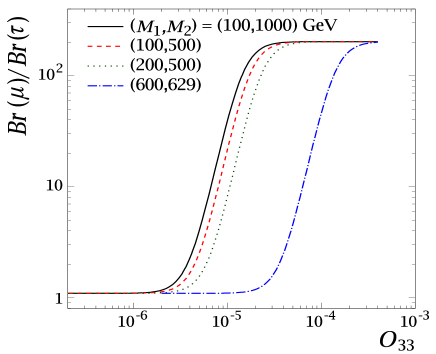
Figure 8: ${Br(h_{1}^{+}\to(\sum_{i}\nu_{i})\mu^{+})}/{Br(h_{1}^{+}\to(\sum_{i}\nu_{i})\tau^{+})}$ as a function of $O_{33}$ and several pairs of $M_{1}$ and $M_{2}$ with $\mu=100\,$GeV. From left to right the curves have $\sin 2\varphi=0.04$, $0.15$, $0.17$ and $0.99$. The dotted line is the same that the curve in the left part of Fig. 6. See text.

The curves in Fig. 6 are basically independent of the value of $\mu$. However, along each curve, smaller values of $O_{33}$ are excluded as $\mu$ decreases. On the other hand they depend on the specific value of $M_{1}$ and $M_{2}$. In fact, as the mixing angle $\sin 2\varphi$ increases the curves are shifted to the right. This is illustrated in Fig. 8 for the small $O_{33}$ case with $f_{12}=0$. All the remaining parameters are chosen as in Fig. 6. In particular the dotted line is the same as the one in Fig. 6.

In summary for the one parameter-solutions we have

$$\left(\frac{m_{\mu}}{m_{\tau}}\right)^{2}\lesssim\frac{Br(h_{1}^{+}\to(\sum_{i}\nu_{i})\mu^{+})}{Br(h_{1}^{+}\to(\sum_{i}\nu_{i})\tau^{+})}\lesssim 10^{4}$$ (55)

We have checked that this result holds for all the parameter space of the NMZM. In particular for $O_{33}$ sufficiently small the charged Higgs decay rate $\Gamma(h^{+}_{1}\rightarrow(\sum_{i}\nu_{i})\mu^{+})$ can be dominant.

7 Conclusions

We have considered the version of the Zee model where both Higgs doublets couple to leptons. Instead of working with all the parameters we have focused on a model with minimal number of couplings consistent with neutrino physics data. We have shown that in the small mixing limit ($\varphi\ll 1$) certain ratios of branching ratios can be used to obtain information about the parameters of the model. Besides the charged Higgs leptonic decays we have also considered the decay $h_{2}^{+}\rightarrow h_{1}^{+}h^{0}$. We have found that this decay, if kinematically allowed, can be used to determine the value of the $\mu$ parameter. Moreover, measurements of $\Gamma(h_{2}^{+}\rightarrow h_{1}^{+}h^{0})$ allow to decide whether the small mixing limit is realized or not.

Assuming that there are no large hierarchies among the couplings $O_{i1}$ ($i=1,2,3$) and $O_{ij}$, and using neutrino physics constraints we have shown that in this scheme only three parameters are independent. We have found that there are four regions, in this three-dimensional parameter space, determined by only $O_{33}$. We have shown that two of these four regions are governed by large values of $O_{33}$ ($10^{-4}-10^{-2}$) while the other two regions are governed by small values of $O_{33}$ ($10^{-7}-10^{-4}$).

We have analysed charged Higgs leptonic decays in the large as well as in the small $O_{33}$ regimes and we have found: (i) in the large $O_{33}$ case, there is a region in which the decays $h_{1}^{+}\rightarrow\nu_{i}\mu^{+}$ and $h_{1}^{+}\rightarrow\nu_{i}\tau^{+}$ are governed by the correponding Yukawas as in the 2HDM of type-I and type-II and another region where the decay $h_{1}^{+}\rightarrow\nu_{i}\mu^{+}$ is enhanced and moreover can be larger than the decay to $h_{1}^{+}\rightarrow\nu_{i}\tau^{+}$. (ii) In the small $O_{33}$ case the decay $h_{1}^{+}\rightarrow\nu_{i}\mu^{+}$ is always enhanced and is larger than the decay $h_{1}^{+}\rightarrow\nu_{i}\tau^{+}$. Therefore we suggest that in order to test the model the decays of the charged Higgs to $\nu_{i}\mu^{+}$ should be searched along with the decays to $\nu_{i}\tau^{+}$. In fact, measurements of the ratio of branching ratios $Br(h_{1}^{+}\to(\sum_{i}\nu_{i})\mu^{+})/Br(h_{1}^{+}\to(\sum_{i}\nu_{i})\tau^{+})$ could give information about what region of this parameter space is realized.

At future colliders the decay channel $\nu\tau^{+}$ is very important for the discovery of charged Higgs bosons [24, 25]. For the LHC and SUSY like 2HDM, it has been claimed that the existence of a relatively heavy charged Higgs bosons, of mass up to 1 TeV, can be probed using the signal $h_{1}^{+}\rightarrow\nu\tau^{+}$ [24]. At future linear colliders a single produced charged Higgs should be associated with the tau and the neutrino coming from the virtual charged Higgs decay [25]. According to our results, and illustrated by Fig. 6, the charged Higgs could emerge from a signal with $\nu_{i}\mu^{+}$ instead of $\nu_{i}\tau^{+}$. Moreover, for a light charged scalar ($M_{1}<m_{t}$) the ratio of branching ratios, $Br(h_{1}^{+}\to(\sum_{i}\nu_{i})\mu^{+})/Br(h_{1}^{+}\to(\sum_{i}\nu_{i})\tau^{+})$ should be measurable.

8 Acknowledgments

We thank W. Porod and E. Nardi for very useful suggestions. Especially to M. Hirsch for his advice as well as for critical readings of the manuscript. D.A. wants to thanks the “Instituto de Física de la Universidad de Antioquia” for their hospitality. This work was supported by Spanish grants BFM2002-00345 and FPA2005-01269. D.A. is supported by a Spanish PhD fellowship by M.C.Y.T. D.R. was partially supported by ALFA-EC funds .

Appendix A The Three-parameter solution

From the set of Eqs. (5.2) we choose to express $f_{12}$, $f_{13}$, $f_{23}$ and $O_{13}$ in terms of $O_{33}$, $O_{22}$, and $O_{12}$

$$f_{12}= -\frac{A}{B}\frac{m_{\tau}\,\sqrt{\Delta m_{23}^{2}}}{m_{\mu}m_{\tau}}\frac{1}{O_{33}}$$ (56)

$$f_{13}= \left[\frac{\frac{m_{\mu}}{m_{\tau}}\left(\frac{\sqrt{2}\,O_{22}}{O_{33}}+\frac{O_{12}\,\left(1+\tan\theta_{23}\right)}{O_{33}\,\tan 2\theta_{12}\,\tan\theta_{23}}\right)-\sqrt{2}}{\kappa\,\,\left(1-\frac{m_{\mu}\,O_{22}}{m_{\tau}O_{33}}\right)\,\left(1+\frac{1}{\tan\theta_{23}}\right)}\right]\frac{\sqrt{\Delta m_{23}^{2}}}{m_{\tau}}\frac{1}{O_{33}}$$ (57)

$$f_{23}= \frac{1}{\kappa\,\left(1-\frac{m_{\mu}\,O_{22}}{m_{\tau}\,O_{33}}\right)\,\tan 2\theta_{12}}\frac{\sqrt{\Delta m_{23}^{2}}}{m_{\tau}}\frac{1}{O_{33}}$$ (58)

$$O_{13}= \frac{2\,\sqrt{2}\,O_{12}\,\tan 2\theta_{12}-O_{22}\,\left(1+\tan\theta_{23}\right)}{2\,\left[\sqrt{2}\,O_{22}\,\tan 2\theta_{12}\,\tan\theta_{23}+O_{12}\,\left(1+\tan\theta_{23}\right)\right]}O_{33}$$ (59)

where

$$A= \left[1+\left(2+4\,\tan^{2}2\theta_{12}\right)\,\tan\theta_{23}+\tan^{2}\theta_{23}\right]$$

$$-2\,\frac{m_{\mu}}{m_{\tau}}\,\tan 2\theta_{12}\,\left[2\,\frac{O_{22}}{O_{33}}\,\tan 2\theta_{12}\,\tan\theta_{23}+\sqrt{2}\,\frac{O_{12}}{O_{33}}\,\left(1+\tan\theta_{23}\right)\right]$$ (60)

$$B= 2\,\kappa\,\left(\frac{m_{\mu}}{m_{\tau}}\,\frac{O_{22}}{O_{33}}-1\right)\,\tan 2\theta_{12}\,\left(1+\tan\theta_{23}\right)$$

$$\times\left[\sqrt{2}\,\frac{O_{22}}{O_{33}}\,\tan 2\theta_{12}\,\tan\theta_{23}+\frac{O_{12}}{O_{33}}\,\left(1+\tan\theta_{23}\right)\right]$$ (61)

References

- [1] K. Eguchi et al. [KamLAND Collaboration], Phys. Rev. Lett. 90, 021802 (2003) [arXiv:hep-ex/0212021].
- [2] S. Fukuda et al. [Super-Kamiokande Collaboration], Phys. Rev. Lett. 86, 5651 (2001) [arXiv:hep-ex/0103032].
- [3] M. Gell-Mann, P. Ramond and R. Slansky, in Supergravity, P. van Nieuwenhuizen & D.Z. Freedman (eds.), North Holland Publ. Co., 1979, Print-80-0576 (CERN); T. Yanagida, in KEK lectures, ed. O. Sawada and A. Sugamoto (KEK, 1979); R. N. Mohapatra and G. Senjanovic, Phys. Rev. Lett. 44, 912 (1980), P. Minkowski, Phys. Lett. B 67, 421 (1977).
- [4] J. Schechter and J. W. F. Valle, Phys. Rev. D 22, 2227 (1980). E. Ma and U. Sarkar, Phys. Rev. Lett. 80, 5716 (1998) [arXiv:hep-ph/9802445].
- [5] L. J. Hall and M. Suzuki, Nucl. Phys. B231, 419 (1984). G. G. Ross and J. W. F. Valle, Phys. Lett. B151, 375 (1985). J. R. Ellis, G. Gelmini, C. Jarlskog, G. G. Ross and J. W. F. Valle, Phys. Lett. B150, 142 (1985).
- [6] M. Hirsch, M. A. Diaz, W. Porod, J. C. Romao and J. W. F. Valle, Phys. Rev. D 62 (2000) 113008 [Erratum-ibid. D 65 (2002) 119901], [arXiv:hep-ph/0004115]. K. Choi, E. J. Chun and K. Hwang, Phys. Lett. B488, 145 (2000), [hep-ph/0005262]. J. M. Mira, E. Nardi, D. A. Restrepo and J. W. F. Valle, Phys. Lett. B 492, 81 (2000)[arXiv:hep-ph/0007266]. K.-m. Cheung and O. C. W. Kong, Phys. Rev. D64, 095007 (2001), [hep-ph/0101347]. T.-F. Feng and X.-Q. Li, Phys. Rev. D63, 073006 (2001), [hep-ph/0012300]. M. Hirsch, Nucl. Phys. Proc. Suppl. 95, 252 (2001). E. J. Chun and S. K. Kang, Phys. Rev. D61, 075012 (2000), [hep-ph/9909429]. E. J. Chun, D.-W. Jung and J. D. Park, hep-ph/0211310. F. Borzumati and J. S. Lee, Phys. Rev. D66, 115012 (2002), [hep-ph/0207184]. E. J. Chun and J. S. Lee, Phys. Rev. D60, 075006 (1999), [hep-ph/9811201]. A. Abada, S. Davidson and M. Losada Phys. Rev. D65, 075010 (2002), [hep-ph/0111332].
- [7] D. Aristizabal Sierra, M. Hirsch, J. W. F. Valle and A. Villanova del Moral, Phys. Rev. D 68, 033006 (2003) [arXiv:hep-ph/0304141].
- [8] A. Zee, Phys. Lett. B 93, 389 (1980) [Erratum-ibid. B 95, 461 (1980)].
- [9] K. S. Babu, Phys. Lett. B 203, 132 (1988).
- [10] L. Wolfenstein, Nucl. Phys. B 175, 93 (1980).
- [11] X. G. He, Eur. Phys. J. C 34, 371 (2004) [arXiv:hep-ph/0307172].
- [12] K. R. S. Balaji, W. Grimus and T. Schwetz, Phys. Lett. B 508, 301 (2001) [arXiv:hep-ph/0104035].
- [13] K. Hasegawa, C. S. Lim and K. Ogure, Phys. Rev. D 68, 053006 (2003) [arXiv:hep-ph/0303252].
- [14] M. Maltoni, T. Schwetz, M. A. Tortola and J. W. F. Valle, New J. Phys. 6, 122 (2004) [arXiv:hep-ph/0405172].
- [15] W. S. Hou, Phys. Lett. B 296, 179 (1992), D. Chang, W. S. Hou and W. Y. Keung; Phys. Rev. D 48, 217 (1993) [arXiv:hep-ph/9302267]; D. Atwood, L. Reina and A. Soni, Phys. Rev. D 55, 3156 (1997) [arXiv:hep-ph/9609279].
- [16] S. Davidson and H. E. Haber, Phys. Rev. D 72, 035004 (2005) [arXiv:hep-ph/0504050].
- [17] A. Heister et al. [ALEPH Collaboration], Phys. Lett. B 543, 1 (2002) [arXiv:hep-ex/0207054].
- [18] G. Abbiendi et al. [OPAL Collaboration], Eur. Phys. J. C 18, 425 (2001) [arXiv:hep-ex/0007040].
- [19] J. Abdallah et al. [DELPHI Collaboration], Eur. Phys. J. C 38, 1 (2004) [arXiv:hep-ex/0410017].
- [20] J. A. Grifols and A. Mendez, Phys. Rev. D 22, 1725 (1980).
- [21] S. Eidelman et al. [Particle Data Group], Phys. Lett. B 592, 1 (2004).
- [22] P. H. Frampton, S. L. Glashow and D. Marfatia, Phys. Lett. B 536, 79 (2002) [arXiv:hep-ph/0201008].
- [23] A. Barroso and P. M. Ferreira, Phys. Rev. D 72, 075010 (2005) [arXiv:hep-ph/0507128].
- [24] D. P. Roy, AIP Conf. Proc. 805, 110 (2006) [arXiv:hep-ph/0510070]; D. P. Roy, Phys. Lett. B 459, 607 (1999) [arXiv:hep-ph/9905542].
- [25] S. Kanemura, S. Moretti and K. Odagiri, JHEP 0102, 011 (2001) [arXiv:hep-ph/0012030].