Dark energy and formation of classical scalar fields

Abstract

We present a quintessence model for the dark energy in which the quintessence scalar field is produced by the decay of a super heavy dark matter and gradually condensate to a classical scalar field. This model can explain both the smallness and the latest observations by WMAP for the equation of state of the dark energy which has $w\sim-1.06$. We review both classical and field theoretical treatment of this model and briefly explain the most important parameters for obtaining the observed characteristic of the dark energy.

1 Introduction

Quintessence models are one the most popular candidates for the dark energy. The main ingredient of these models is a classical scalar field. It is not difficult to find scalar particles/quantum fields in the Standard Model and its extension, and in cosmological context. But it is evident to find a field with necessary characteristics. Some authors have suggested the same field as the driver force behind inflation and dark energyinfquin . The common aspect of these models is a non-zero slowly decreasing classical potential during inflation era which at late time settles to a very small value and behaves as the dark energy today. Even without direct relation to inflaton, most of other quintessence models also predict a late time tracker classical scalar field with a potential which in one way or another gets a small but non-zero value at late times. As for the particle physics of these models, all extensions of the Standard Model include various types of scalar fields, from very light ones such as QCD axion, dilaton, and modulies in string theories, to presumably heavy particles such as super partner of spinor in supersymmetry models and Higgs bosons.

There are however one problematic issue regarding the mass of quintessence fields. In most quintessence models as the classical scalar field is related to the phenomena at very high energies, it is difficult to make its value very small without extreme fine-tuning. For this reason its mass and coupling must be small, in most cases of order $\sim 10^{-32}eV$ or it must have tachyonic potential - a potential with a negative effective mass such that the mass and interaction term cancel each other. It is not easy to incorporate such a small mass into particle physics models. In most cases radiative corrections make the bare small mass much larger than what is neededmassrenor . Exceptional cases exist in which due to a translation symmetry a pseudo-Nambu-Goldstone boson does not get correction after renormalisation and can keep is smallnessquinpngb . The form of their potentials is not however very simple and it is not sure if they can be easily obtained from particle physics model without fine-tuning or additional concepts which are yet more sophisticated. This type of modelling just shift an unexplained problem to another one and does not seem to be a concrete solution of the problem. In addition, the latest results from WMAPwmap shows that the simplest inflation model with just a mass term in the potential is the best fit to the CMB anisotropy data. If this conclusion is confirmed, models which try to unify quintessence field with inflaton would be compromised or at least will have more difficulties to explain the late behaviour of this field. It would not be easy to explain a very small but non-zero value for the field with such a simple potential unless other ingredients and most probably some fine-tuning be added to the models.

There is also an unexplored issue regarding the formation of a classical scalar field and its potential. Although a large number of quantum scalar fields are predicted by particle physics models, their condensation to a classical field is not a trivial process specially when complex potentials are requested for quintessence models. The importance of condensation is not limited to the quintessence models of dark energy and is an indispensable content of Higgs phenomena, symmetry breaking and phase transition in the context of baryo and lepto genesis, electroweak and QCD.

Here we first review a quintessence model based on the condensation of a light scalar produced by slow decay of a heavy dark matter and show that it can explain the observation of $w\lesssim-1$ for the equation of state of the dark energy. We also review the methodology and some analytical results of the field theoretical study of the condensation process and discuss important parameters for its formation and evolution.

2 A meta-stable super heavy dark matter

The motivation for this type of dark matter is the observation of Ultra High Energy Cosmic Rays (UHECR)uhecr . Acceleration models have great difficulties to produce enough particles at these huge energies - larger than $\sim 10^{20}eV$. Moreover, the sites of the potential accelerators, magnetars and AGNs, which are marginally capable of accelerating charged particles to such energies must be close - in a distance $<50~{}Mpc$ - otherwise the interaction with the CMB decelerates nucleons. This process should make what is called GZK cutoff in the high energy tail of the cosmic rays spectrum and has been predicted in 1960s, but is not observed. Considering the small fluxes which can be provided by each source at these energies, it does not seem that there are enough sources in the limited volume space permitted by the CMB above to explain the observed spectrum by standard Fermi acceleration or its improvement by taking into account non-linear effects e.g Alfven shocks.

Top-down modelstopdown as the origin of UHECR considers the decay of a meta-stable super heavy particle particle (here on called $X$) as the sources of (anti)-nucleons producing the high energy shower in the Earth atmosphere. In this case the contribution of the halo of the Galaxy is much more important than cosmological onesxx houriwimpzilla . A detail calculation of energy dissipation of high energy particles show that for $m_{x}\sim 10^{22}-10^{24}eV$ and lifetimes even as short as $\sim 10\tau_{0}$ where $\tau_{0}$ is the present age of the Universe, roughly the totality of dark matter can be $X$ particles without violating the present observations of the UHECR fluxhouriwimpzilla .

There are a number of particle physics candidates for $X$ particles. In models inspired by string theory and various possible compactifications, meta-stable particle called crypton with a mass $\sim 10^{22}eV$ or higher can be $X$ particlescrypton . Observation of neutrino oscillation and the limit on their masses $\sum m_{\nu}<0.68eV$wmap along with the close to degeneracy of their mass difference $\Delta m^{2}\approx 10^{-}3$ makes seesaw mechanism the most favourite model for explaining these observations. In this case, the small mass of left neutrinos push the mass of right hand neutrinos to $~{}10^{23}eV$ or higher. In supersymmetric models seesaw can also exist in the super-partner sector of neutrinos and if some of right hand sneutrinos are meta-stable due to discrete global symmetries, they can be also good candidates for $X$ particlesrnu .

Besides explaining the mystery of UHECRs, a meta-stable dark matter can also solve another mystery: a $w\lesssim-1$ for the dark energy where $w=p/\rho$ with $p$ and $\rho$ respectively pressure and density of dark energy. An ordinary quintessence model based on a scalar field with positive kinetic energy has always $w\geqslant-1$ and therfore can not explain the observed equation of state of the dark energy if $w\lesssim-1$ is confirmed. Nonetheless, it is possible to show that in presence of cosmological constant i.e. when $w=-1$ and a slowly decayinghouriustate (or interactingquindmint ) dark matter, if supernovae data is analysed with prior assumption of stable dark matter, an effective $w\leqslant-1$ will be obtained. To prove this, we use an approximation solution of the expansion equation:

$$H^{2}(z)=\frac{8\pi G}{3}T^{00}(z)+\frac{\Lambda}{3}$$ (1)

where H is the Hubble constant and $T^{\mu\nu}$ is the energy-momentum tensor of the Universe and $T^{00}=\rho$. We want to find an analytical expression for the equivalent quintessence model with a stable dark matter to a cosmology with a decaying dark matter of lifetime $\tau$ and a cosmological constant $\Lambda$. With a good precision the total density of such models can be written as the following:

$$\frac{\rho(z)}{{\rho}_{c}}\approx{\Omega}_{M}(1+z)^{3}\exp(\frac{{\tau}_{0}-t}{\tau})+{\Omega}_{Hot}(1+z)^{4}+{\Omega}_{M}(1+z)^{4}\biggl{(}1-\exp(\frac{{\tau}_{0}-t}{\tau})\biggr{)}+{\Omega}_{\Lambda}.$$ (2)

We assume a flat cosmology i.e. ${\Omega}_{M}+{\Omega}_{\Lambda}=1$ (ignoring the hot part). ${\rho}_{c}$ is the present critical density. If the dark matter is stable and we neglect the contribution of hot component, the expansion factor $a(t)$ is:

$$\frac{a(t)}{a({\tau}_{0})}=\biggl{[}\frac{(B\exp(\alpha(t-{\tau}_{0}))-1)^{2}}{4AB\exp(\alpha(t-{\tau}_{0}))}\biggr{]}^{\frac{1}{3}}\equiv\frac{1}{1+z}.$$ (3)

$$A\equiv\frac{{\Omega}_{\Lambda}}{1-{\Omega}_{\Lambda}}\quad,\quad B\equiv\frac{1+\sqrt{{\Omega}_{\Lambda}}}{1-\sqrt{{\Omega}_{\Lambda}}}\quad,\quad\alpha\equiv 3H_{0}\sqrt{{\Omega}_{\Lambda}}$$ (4)

Using (3) as an approximation for $\frac{a(t)}{a({\tau}_{0})}$ when dark matter decays, (2) takes the following form:

$$\frac{\rho(z)}{{\rho}_{c}} \approx {\Omega}_{M}(1+z)^{3}C^{-\frac{1}{\alpha\tau}}+{\Omega}_{Hot}(1+z)^{4}+{\Omega}_{M}(1+z)^{4}(1-C^{-\frac{1}{\alpha\tau}})+{\Omega}_{\Lambda}$$ (5)

$$C \equiv \frac{1}{B}\biggl{(}1+\frac{4A}{(1+z)^{3}}-\sqrt{(1+\frac{4A}{(1+z)^{3}})^{2}-1}\biggr{)}$$ (6)

where $\alpha\tau\gg 1$ and (5) becomes:

$$\frac{\rho(z)}{{\rho}_{c}} \approx {\Omega}_{M}(1+z)^{3}+{\Omega}_{Hot}(1+z)^{4}+{\Omega}_{q}(1+z)^{3{\gamma}_{q}},$$ (7)

$${\Omega}_{q}(1+z)^{3{\gamma}_{q}} \equiv {\Omega}_{\Lambda}(1+\frac{{\Omega}_{M}}{\alpha\tau{\Omega}_{\Lambda}}z(1+z)^{3}\ln C)$$ (8)

Equation (8) is the definition of equivalent quintessence model. After linearising this expression we find:

$$w_{q}\equiv{\gamma}_{q}-1\approx\frac{{\Omega}_{M}(1+4A)(1-\sqrt{2A})}{3\alpha\tau{\Omega}_{\Lambda}B}-1$$ (9)

Using (9), one can show that if $w_{q}<-1$ if ${\Omega}_{\Lambda}>\frac{1}{3}$. In the general case of an interaction between dark matter and dark energy, the exponential term in (2) can be replaced by a more general expression $f(z)$ which presents the modification of the density of both component due to their interaction. It has been shownquindmint that this function can be selected in such a way that $w_{q}<-1$.

A more precise treatment of this model needs the simulation of the decay and the dynamics of of the remnant. This has been done for various values of the cosmological parameters as well as mass and lifetime of the dark matterhouriustate and the results has been used to fit this model to supernovae data. The best fit of this model for fixed $\tau=5\tau_{0}$ predicts following values for other parameters:

$$H_{0}=68.4\quad,\quad\Omega_{\Lambda}=0.73,\quad\Omega_{q}=0.69\quad,\quad w=-1.066$$ (10)

These values are very close to the latest results from combined WMAP, SNLS and SDSS. The importance of this result is specially in the fact that the value for $\tau$, the lifetime of the dark matter, comes from a completely different data set i.e. the flux of UHECR. This parameter is very important for the effect of the decay on the equation of state of the dark energy. For instance, if $\tau=50\tau_{0}$, $w=-1.006$ i.e. much closer to the cosmological constanthouriustate . Therefore, this model has not been fine-tuned to obtain the observed value of $w$ as most of other models for having $w\lesssim-1$ (what is called phantom models) are.

3 Dark energy from a decaying dark matter

The question that arises now is whether dark energy can be related to the decay of the dark matter too. The reason for such idea is the coincidence problem. We don’t have any explanation why the energy density of the dark matter and dark energy is so highly fine-tuned in the early universe - by a factor of $\sim 10^{30}$ or more, depending on the time of their production - such that they become comparable only after galaxy formation. The most trivial answer to this question is evidently that somehow there is a relation between these two main contents of the Universeinterac0 . The nature of their relation however should be in such a way that the mentioned fine-tuning appears as natural.

In the models with meta-stable, if the dark energy or more precisely the quintessence field is produced by the slow decay of the dark matter and if it is produced in enough small amount, its density can be small and its relation with the dark matter solves the coincidence problemhouridmquin . We should also remark that when we say it must be produced in small amount, this looks like a fine-tuning which we want to avoid. However, here the branching ratio of the heavy dark matter to dark energy is orders of magnitude larger than in usual quintessence models. The reason is the long life of the dark matter. Observationally speaking, the estimation of these quantities come from completely different data sets - the lifetime of the dark matter and the range of its mass is set by the observed flux of the ultra high energy cosmic rays. As we discussed in the previous section, in the top-down models the contribution of the Galactic halo is much larger than cosmic one. It is a local process and therefore independent of the cosmological parameters. The smallness of dark energy is thus partially due to the long lifetime of the dark matter. Below we will see that branching ratio of dark matter to dark energy becomes similar to other weak interactions and can be studies in the frame of present particle physics models such as supersymmetry and supergravity.

In a simple realization of such a model the Lagrangian has the following form:

$${\mathcal{L}}=\int d^{4}x\sqrt{-g}\biggl{[}\frac{1}{2}g^{\mu\nu}{\partial}_{\mu}{\phi}_{x}{\partial}_{\nu}{\phi}_{x}+\frac{1}{2}g^{\mu\nu}{\partial}_{\mu}\Phi{\partial}_{\nu}\Phi-V({\phi}_{x},\Phi,A)\biggr{]}+{\mathcal{L}}_{A}$$ (11)

${\phi}_{x}$ presents the meta-stable dark matter and $\Phi$ the quintessence. For simplicity we assume that it is a scalar, but general aspects of the model will be the same if it is a spinor. The field $A$ presents collectively other fields. The term $V({\phi}_{x},\Phi,A)$ includes all interactions including self-interaction potential for ${\phi}_{x}$ and $\Phi$:

$$V({\phi}_{x},\Phi,J)=V_{q}(\Phi)+V_{x}({\phi}_{x})+g{{\phi}_{x}}^{m}{\Phi}^{n}+W({\phi}_{x},\Phi,J)$$ (12)

The term $g{{\phi}_{x}}^{m}{\Phi}^{n}$ is responsible for the annihilation of $X$ and back reaction of quintessence field on the dark matter. The potential $W({\phi}_{x},\Phi,A)$ presents interactions which contribute to the decay of $X$ to light fields and to $\Phi$ (in addition to what is shown explicitly in (12)). The very long lifetime of $X$ constrains this term and $g$. They must be strongly suppressed. For $n=2$ and $m=2$, the interaction term contributes to the mass of ${\phi}_{x}$ and $\Phi$. Because of the huge mass of ${\phi}_{x}$ (which must come from another coupling) and its very small occupation number:

$$<{{\phi}_{x}}^{2}>\sim 2{\rho}_{x}/{m_{x}}^{2}$$ (13)

For sufficiently small $g$ the effect of this term on its mass is very small.

We assume that $X$ particles don’t have self-interaction i.e. $V_{x}({\phi}_{x})=0$ and $V_{q}(\Phi)$ is a polynomial, in simplest case containing only a mass term and $\Phi^{4}$ self-interaction with a coupling $\lambda$. At classical level we replace ${\phi}_{x}$ and $A$ with their density using (13). With these simplifications, the evolution equations for the classical components are:

$$\dot{\varphi}[\ddot{\varphi}+3H\dot{\varphi}+{m_{\Phi}}^{2}\varphi+\lambda{\varphi}^{3}] = -2g\dot{\varphi}\varphi\biggl{(}\frac{2{\rho}_{x}}{{m_{x}}^{2}}\biggr{)}+{\Gamma}_{\Phi}{\rho}_{x}$$ (14)

$$\dot{{\rho}_{x}}+3H{\rho}_{x} = -({\Gamma}_{\Phi}+{\Gamma}_{A}){{\rho}_{x}}-{\pi}^{4}g^{2}\biggl{(}\frac{{{\rho}_{x}}^{2}}{{m_{x}}^{3}}-\frac{{{\rho}_{q}}^{\prime 2}}{{m_{q}}^{3}}\biggr{)}$$ (15)

$$\dot{{\rho}_{A}}+3H({\rho}_{A}+P_{A}) = {\Gamma}_{A}{{\rho}_{x}}$$ (16)

where $\varphi$ is the classical component of $\Phi$ and ${\Gamma}_{\Phi}$ and ${\Gamma}_{A}$ are the decay width of $X$ particles to $\Phi$ and $A$ respectively.

Numerical solution of these equations along with Einstein equations for typical values of the parameters show that in such models the classical field behaves like a cosmological constant - after few orders of magnitude in redshift from the end of $X$ production, presumably after reheating, its density approaches a constant and it keeps this behaviour until present, see Fig.1. Variation of parameters by few orders of magnitudes does not change the general aspect of $\varphi$ evolution, see Fig.2-(a) and (b). Therefore this model is not fine-tuned.

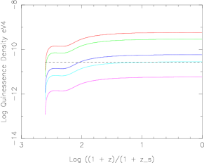
Figure 1: Evolution of quintessence field density for ${\Gamma}_{0}=1/\tau_{0}\equiv{\Gamma}_{\Phi}/\Gamma=10^{-16}$ (magenta), $5{\Gamma}_{0}$ (cyan), $10{\Gamma}_{0}$ (blue), $50{\Gamma}_{0}$ (green), $100{\Gamma}_{0}$ (red). Dash line is the observed value of the dark energy. $m_{\Phi}=10^{-6}eV$, $\lambda=10^{-20}$.

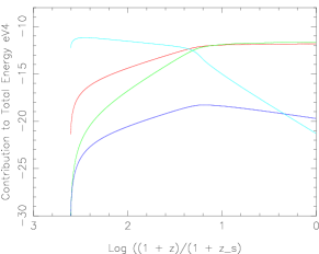
(a) (b)

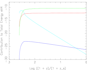
Figure 2: Evolution of the contribution to the energy density of $\varphi$ for ${\Gamma}_{0}\equiv{\Gamma}_{q}/\Gamma=10^{-16}$ and : Left, $m_{q}=10^{-8}eV$ and $\lambda=10^{-20}$; Right, $m_{q}=10^{-6}eV$ and $\lambda=10^{-10}$.Curves are: mass (red), self-interaction (green), kinetic energy (cyan) and interaction with super heavy dark matter (blue).

4 Formation of a classical field

The results of the previous section are obtained for a classical field. In the Nature however all the particles and fields have quantum behaviour. Decoherence can make particles to behave semi-classically, i.e. have a wave function restricted spatially and in momentum space. A classical field however is more complex and classical behaviour of particles does not necessarily means a collective behaviour as a classical field. Therefore, in a more rigorous treatment of the model of the previous section, we must begin with the corresponding quantum field theory, calculate quantum expectations and see if these expectations which are equivalent to the classical fields behave as requested for a dark energy.

The classical field is defined as the expectation value of the quantum field:

$$\varphi(x)\equiv\langle\Psi|\Phi(x)|\Psi\rangle$$ (17)

where $|\Psi\rangle$ is an element of the Fock space of the system. It is also called a condensate in analogy with quantum mechanics. Using canonical representation of the field $\Phi$, it is easy to see that for a free quantum scalar field $\langle\Psi|\Phi|\Psi\rangle=0$. Therefore, a necessary condition for appearance of a classical scalar field is interaction. The detail study of the Lagrangian (11) needs an explicit definition of interaction/decay term. We consider following decay modes for $X$ particles:

$$(a)\quad\quad\quad\quad\quad\quad\quad \quad\quad\quad\quad\hskip 28.45274pt\text{or}~{}~{}(b)$$

(18)

By considering two modes we can investigate how the type of interactions in the model can change the outcome for the classical field.

After adding the corresponding interaction term to the Lagrangian and neglecting the quadratic interaction between $X$ and $\Phi$, we find following equations for the evolution of the classical field $\varphi$:

$$\frac{1}{\sqrt{-g}}{\partial}_{\mu}(\sqrt{-g}g^{\mu\nu}{\partial}_{\nu}\varphi)+m_{\Phi}^{2}\varphi+\frac{\lambda}{n}\sum_{i=0}^{n-1}(i+1)\binom{n}{i+1}{\varphi}^{i}\langle{\phi}^{n-i-1}\rangle-\mathsf{g}\langle XA^{2}\rangle=0$$

For ((18))-a (19)

$$\frac{1}{\sqrt{-g}}{\partial}_{\mu}(\sqrt{-g}g^{\mu\nu}{\partial}_{\nu}\varphi)+m_{\Phi}^{2}\varphi+\frac{\lambda}{n}\sum_{i=0}^{n-1}(i+1)\binom{n}{i+1}{\varphi}^{i}\langle{\phi}^{n-i-1}\rangle-2\mathsf{g}\varphi\langle XA\rangle-2\mathsf{g}\langle\phi XA\rangle=0$$

For ((18))-b (20)

where $\phi$ is the quantum component of $\Phi$ with a null expectation value. The next step in this calculation is determination of expectation values in (19) and (20). The easiest method for this purpose is Schwinger closed time path (CTP) formalism. The detail of this calculation can be found in Ref.houridecohere . Here we briefly discuss some of the results and prospects for future studies.

Considering only a mass term in the potential of $\Phi$ field, at radiation domination epoch after reheating the general solutions of the equations (19) and (20) at the WKB approximation level are:

$$\chi(\eta) = \chi_{1}D_{q}(\alpha_{\Phi}\eta)+\chi_{2}D_{q}(-\alpha_{\Phi}\eta)+g\int_{\eta_{0}}^{\eta}d\eta^{\prime}\langle\mathtt{X}\mathtt{A}^{2}\rangle G^{\chi}(\eta,\eta^{\prime})\quad\quad\text{For decay mode $(a)$}$$ (21)

$$\chi(\eta) = \chi^{{}^{\prime}}_{1}D_{q}\biggl{(}\alpha_{\Phi}\int d\eta(1-\frac{2g\langle\mathtt{X}\mathtt{A}\rangle}{a^{2}m^{2}_{\Phi}})^{\frac{1}{4}}\biggr{)}+\chi^{{}^{\prime}}_{2}D_{q}\biggl{(}-\alpha_{\Phi}\int d\eta(1-\frac{2g\langle\mathtt{X}\mathtt{A}\rangle}{a^{2}m^{2}_{\Phi}})^{\frac{1}{4}}\biggr{)}+$$ (22)

$$2g\int_{\eta_{0}}^{\eta}d\eta^{\prime}\langle\Upsilon\mathtt{X}\mathtt{A}\rangle G^{\chi}(\eta,\eta^{\prime})\quad\quad\text{For decay mode $(b)$}$$

$$\alpha_{\Phi}\equiv(1+i)\sqrt{B_{\Phi}}\quad q\equiv-\frac{1+\frac{ik^{2}}{B_{\Phi}}}{2}\quad B_{\Phi}\equiv\frac{a_{0}m_{\Phi}}{\eta_{0}}=\frac{m_{\Phi}}{H_{0}\eta_{0}^{2}}=a^{2}_{0}H_{0}m_{\Phi}$$ (23)

$$\chi\equiv a\varphi\quad\Upsilon\equiv a\phi\quad\mathtt{X}\equiv aX\quad\mathtt{A}\equiv aA$$ (24)

where $\chi_{1}$, $\chi_{2}$, $\chi^{{}^{\prime}}_{1}$ and $\chi^{{}^{\prime}}_{2}$ and integration constants. $D_{q}$ is the parabolic cylindrical function. Expectation values in (21) and (22) include integration over multiple $D_{q}$ functions and don’t have a closed analytical expressions. Using the asymptotic behaviour of $D_{q}(z)$ at large $z$, one finds that for both decay modes (a) and (b), the homogeneous part of the solutions (21) and (22) is proportional to $\eta^{-1/2}$ and therefore deceases with time.

In the same way, we can find the time dependence of the special solution. For large $\eta$ it is proportional to $\eta^{2+\epsilon}$ for both decay modes. The parameter $\epsilon$ is added by hand to present the unknown time variation of the cosmological state $|\Psi\rangle$. Although in this formalism no explicit reference to time dependence of $|\Psi\rangle$ is made, its definition as the quantum state of particle in an expanding and evolving universe has implicitly the concept of time dependence in it. $\epsilon$ presents the back-reaction of interactions and expansion on the quantum state of the Universe. In classical treatment of particle production a dissipation term is usually added to express this back-reactionbackreact . In a field theoretical analysis of this problem the addition of a term by hand is not allowed and a more rigorous strategy must be taken.

In comoving coordinates the classical field $\varphi=\chi/a$ and varies as:

$$\varphi\propto t^{-1/2+2+\epsilon} m\neq 0$$ Assuming for all fields, both decay modes. (25)

$$\varphi\propto t^{-1/2+3+\epsilon} m_{\Phi}\approx 0$$ For and mode (b). (26)

For all cases, the late time behaviour of $\varphi$ depends on $\epsilon$ i.e. the back reaction and must be calculated numerically. We expect that $\epsilon$ depends on the density and lifetime of $X$ field, and on the expansion of the Universe. However, at late times when the energy density of the dark matter $X$ becomes comparable to the density of the dark energy $\sim 1/2m_{\Phi}^{2}\varphi^{2}$, there is a strong feedback between expansion rate and the density of dark matter - higher expansion brings down the density of the dark matter and therefore the rate of $\varphi$ production per unit of volume decreases. This reduces the density of the dark energy and the expansion. We have seen the same feedback in the classical formulation of this model in the previous section.

Finally it can be shown that $k$ dependence of $\varphi$ approaches a constant value at large scales consistent with observations of the dark energy.

5 Conclusion

The nature of dark matter and dark energy, along with search for a quantum theory of gravity are the greatest mysteries of contemporary physics. The can be related the first two can help - at least we hope - the third one which is more abstract and less available to cosmological observation or experiment in high energy accelerators.

Although numerous models for dark energy are proposed, the mere observation of its equation of state, whatever precise, can not distinguish between many of these models. Therefore one should find a relation between these models and other phenomena with independently quantities to be able to discriminate the right model.

Here we suggested a relation between dark matter and dark energy and fixed the properties of the model using completely independent observable: flux of the ultra high energy cosmic rays and supernovae observations. The closeness of predicted values in (10) to more recent observations is not a proof of the correctness of all aspects of this model. But maybe it is an indicator of the right way to proceed to the final solution.

References

- (1) D. Suematsu, J. Cosmol. Astrop. Phys. 0601, 2006 (026), astro-ph/0511742.
- (2) D.J.H. Chung, L.L. Everett, A. Riotto, Phys. Lett. B 556, (2003) (61) hep-ph/0210427.
- (3) J.A. Frieman, et al., Phys. Rev. Lett. 75, 1995 (2077), Y. Nomura, et al., Phys. Lett. B 484, 2000 (103), hep-ph/0004182, K. Choi, PRD 62, 2000 (043509), C.T. Hill, A.K. Leibovich, Phys. Rev. D 66, 2002 (075010), hep-ph/0205237, , L.J. Hall, Y. Nomura, S.J. Oliver, Phys. Rev. Lett. 95, 2005 (141302), astro-ph/0503706, N. Kaloper, L. Sorbo, asto-ph/0511543.
- (4) D.N. Spergel et al., March 2006, http://lambda.gsfc.nasa.gov.
- (5) Bird D.J. et al., ApJ. 424, 491 (1994), Hayashida N. et al., Phys. Rev. Lett. 73, 3491 (1994), Yoshida S. et al., Astropart. Phys. 3, 105 (1995), (See F. Halzen, D. Hooper, Rept. Prog. Phys. 65, (2002) (1025), astro-ph/0204527 for review).
- (6) Bhattacharjee P., Hill C.T., Schramm D.N., Phys. Rev. Lett. 69, 567 (1992).
- (7) Berezinsky V., Kachelrie & Vilenkin A., Phys. Rev. Lett. 79, 4302 (1997).
- (8) H. Ziaeepour, Astropart. Phys. 16, (2001) (101), astro-ph/0001137.
- (9) Ellis J., Lopez J.L., Nanopoulos D.V. Phys. Lett. B2453751990, Benakli K. et al., Phys. Rev. D 59, 047301 (1999).
- (10) T. Asaka, K. Ishiwata, T. Moroi, hep-ph/0512118, S. Gopalakrishna, A. de Gouvêa, hep-ph/0602027.
- (11) H. Ziaeepour, “Cosmic Equation of State, Quintessence and Decaying Dark Matter”, astro-ph/0002400.
- (12) S. Das, P.S. Corasaniti, J. Khoury, “Super-accelerati on as Signature of Dark Sector Interaction”, astro-ph/0510628.
- (13) L.P. Chimento, A.S. Jakubi, D. Pavòn, W. Zimdahl, Phys. Rev. D 67, (2003) (083513) astro-ph/0303145, L.P. Chimento, A.S. Jakubi, D. Pavòn, Phys. Rev. D 67, (2003) (087302) astro-ph/0303160.
- (14) H. Ziaeepour, Phys. Rev. D 69, 2004 (063512), astro-ph/0308515, H. Ziaeepour, in “Progress in Dark Matter Research”, Nova Science Inc. New York (2005) p. 175, astro-ph/0406079.
- (15) H.Ziaeepour, hep-ph/0603125.
- (16) A.D. Doglov, S.H. Hansen, Nucl. Phys. B 548, 1998 (408), hep-ph/9810428.