Single Transverse-Spin Asymmetry in Drell-Yan Production
at Large and Moderate Transverse Momentum

Abstract

We study the single-transverse spin asymmetry for the Drell-Yan process. We consider production of the lepton pair at large transverse momentum, $q_{\perp}\sim Q$, where $Q$ is the pair’s mass. The spin asymmetry is then of higher twist and may be generated by twist-three quark-gluon correlation functions. Expanding the result for $q_{\perp}\ll Q$, we make contact with the transverse-momentum-dependent QCD factorization involving the so-called Sivers functions. We find that the two mechanisms, quark-gluon correlations on one hand and the Sivers effect on the other, contain the same physics in this region. This ties the two together and imposes an important constraint on phenomenological studies of single transverse spin asymmetries.

I Introduction

Single-transverse spin asymmetries (SSAs) play an important role for our understanding of QCD and of nucleon structure. They have a long history, starting from the 1970s and 1980s when surprisingly large SSAs were observed in hadronic reactions such as $p^{\uparrow}p\to\pi X$ at forward angles of the produced pion E704-Bunce . The last few years have seen a renaissance in the experimental studies of SSAs. The HERMES collaboration at DESY, SMC and COMPASS at CERN, and the CLAS collaboration at the Jefferson Laboratory have investigated SSAs in semi-inclusive hadron production $eN^{\uparrow}\to e\pi X$ in deep-inelastic scattering dis . For proton targets, remarkably large asymmetries were found. The advent of the first polarized proton-proton collider, RHIC, has opened new possibilities for extending the studies of SSAs in hadronic scattering into a regime where the use of QCD perturbation theory in the analysis of the data appears to be justified. The STAR, PHENIX and BRAHMS collaborations have presented data for single-inclusive hadron production, and large single-spin effects at forward rapidities were found to persist to RHIC energies rhic .

The observed large size of SSAs in hadronic scattering has presented a challenge for QCD theorists review . Two mechanisms have been proposed Siv90 ; Efremov ; qiu and been extensively applied qiu ; Kanazawa:2000hz ; Ans94 ; MulTanBoe ; siverscompare in phenomenological studies. The first relies on the use of transverse-momentum dependent parton distributions for the transversely polarized proton. For these distributions, known as Sivers functions Siv90 , the parton transverse momentum is assumed to be correlated with the proton spin vector, so that spin asymmetries naturally arise from the directional preference expressed by that correlation. The other mechanism (referred to as Efremov-Teryaev-Qiu-Sterman (ETQS) mechanism) is formulated in terms of the collinear factorization approach and twist-three transverse-spin-dependent quark-gluon correlation functions of the proton Efremov ; qiu .

A concept common to both mechanisms is the factorization of the spin-dependent cross section into functions describing the distributions of quarks and gluons in the polarized proton, and partonic hard-scattering cross sections, calculated in QCD perturbation theory. The question of which mechanism should be used in the analysis of a single-spin asymmetry is therefore primarily tied to the factorization theorem that applies for the single-spin observable under consideration. For example, for the single-inclusive process $p^{\uparrow}p\to\pi X$, there is only one hard scale, the transverse momentum $p_{T}$ of the produced pion, and the SSA is power-suppressed (“higher-twist”) by $1/p_{T}$. In this case, one can prove a collinear factorization theorem in terms of the quark-gluon correlation functions qiu , and the ETQS mechanism applies. On the other hand, the observables typically investigated in deep-inelastic lepton scattering (DIS) are characterized by a large scale $Q$ (the virtuality of the DIS photon) and by the much smaller, and also measured, transverse momentum $q_{\perp}$ of the produced hadron. In this two-scale case, single-spin asymmetries may arise at leading twist, i.e., not suppressed by $1/Q$. The relevant factorization theorem is formulated in terms of transverse-momentum-dependent (TMD) functions ColSop81 ; ColSopSte85 ; JiMaYu04 ; ColMet04 , in particular the Sivers functions. We note that much progress has been made recently in understanding the underlying theoretical issues in the TMD QCD factorization. For example, the gauge-invariance properties of the necessary TMD parton distributions have been clarified BroHwaSch02 ; Col02 ; BelJiYua02 ; BoeMulPij03 for DIS and Drell-Yan processes, and an extension to more complicated hadronic processes has been considered in Pijl .

From what we just discussed, the two mechanisms for single-spin asymmetries might appear to be essentially unrelated. However, one can make an argument that a consistent theoretical description of the SSA for a hard process over its full kinematical regime requires both mechanisms to be present and to contain the same physics in the region where they both apply. To give a specific example – which will in fact be the example treated in this paper – let us consider the SSA for the Drell-Yan process when the invariant mass $Q$ of the pair as well as its transverse momentum $q_{\perp}$ are measured. We stress that we consider cross sections differential just in $Q^{2}$ and $q_{\perp}$, but not specifically in the angular distributions of any of the individual leptons.

At relatively large pair transverse momentum, $q_{\perp}\sim Q$, there is only one large scale, and the SSA will be power-suppressed in that scale. This directs us to use the ETQS mechanism with its collinear factorization involving the twist-three quark-gluon correlation functions and corresponding hard-scattering functions calculated at lowest order from partonic $3\to 2$ processes. As an aside, when taking the real-photon ($Q^{2}\to 0$) limit, this calculation will yield the result for the SSA in direct-photon production qiu .

We can next investigate what happens when we make the ratio $q_{\perp}/Q$ small, keeping both scales perturbative, $Q\gg q_{\perp}\gg\Lambda_{\rm QCD}$. We refer to $q_{\perp}$ in this regime as “moderate” transverse momentum. The ETQS mechanism will still apply here (even though the hard-scattering functions will develop large logarithms of the ratio $q_{\perp}/Q$ that will eventually need to be resummed to all orders in the strong coupling). At the same time, however, the factorization in terms of TMD distributions applies now ColSop81 ; ColSopSte85 ; JiMaYu04 , which involves the Sivers functions. If both mechanisms are internally consistent, they must describe the same physics in this region.

In a recent publication JiQiuVogYua06 , we have demonstrated that the two mechanisms indeed provide the same description of the single-spin asymmetry for the Drell-Yan process in the regime $\Lambda_{\rm QCD}\ll q_{\perp}\ll Q$, and that there is a direct correspondence between the Sivers functions and the twist-three quark-gluon correlation functions, derived also earlier in BoeMulPij03 . The key observation is that, at moderate transverse momentum, the Sivers function may be calculated perturbatively, using the twist-three quark-gluon correlation functions. In other words, the ETQS mechanism generates a non-vanishing Sivers function in this kinematic regime. Although there have been earlier efforts to link the two mechanisms BoeMulPij03 ; MaWa03 ; bacchetta , a clear connection, at the level of physical observables, has been established only in JiQiuVogYua06 . In the present paper, we present details of the derivation of our results in JiQiuVogYua06 .

Our results may in some sense be viewed as establishing a unification of the two mechanisms. At large $q_{\perp}$, the ETQS mechanism applies. At moderate transverse momentum, a smooth transition from the ETQS mechanism to the one based on TMD factorization occurs, with the two approaches containing the same physics. At yet lower $q_{\perp}$ ($\sim\Lambda_{\rm QCD}$), the TMD factorization still applies, containing in a natural way the transition from perturbative to non-perturbative physics. We believe that this unified picture should prove to be the best approach to phenomenological studies of SSAs.

The remainder of the paper is organized as follows. In Sec. II, we introduce the twist-three quark-gluon correlation function and explain its physical significance. In Sec. III, we calculate the single-spin differential cross section for Drell-Yan production using the ETQS mechanism, and we study its limit $q_{\perp}\ll Q$ in Sec. IV. A comparison with the TMD factorization approach is made in Sec. V, and we conclude the paper in Sec. VI.

II Transverse-Spin-Dependent Quark-Gluon Correlation

Consider a transversely polarized proton traveling at nearly the speed of light. Its internal color electric and magnetic fields then have preferred orientations in the plane transverse to the proton’s direction of motion. By parity invariance, the color electric field must be orthogonal to the spin of the proton. If averaged over the proton wave function, the field vanishes because the proton is color-neutral (and also because of time-reversal symmetry). However, if one multiplies the color field with the quark color current, the average may be non-zero. This average defines a quark-gluon correlation function that characterizes a property of a polarized proton. In some sense, the correlation describes how strongly polarized the color electric field is in a spinning proton.

In this paper, we are mostly interested in the so-called light-cone correlations. For these, quark and/or gluon fields are separated along the light-cone direction $\xi^{-}$ (if $\xi^{\mu}$ denotes a space-time coordinate, the light-cone variables are defined as $\xi^{\pm}=(\xi^{0}\pm\xi^{3})/\sqrt{2},\xi_{\perp}=(\xi^{1},\xi^{2})$). It is the light-cone correlations that characterize the structure of the proton in high-energy scattering. One finds the following expression for the spin-dependent quark-gluon correlation described above qiu :

$$\Phi_{F}^{\alpha}(k_{q1}^{+},k_{q2}^{+})^{a}_{ij} = \int\frac{d\zeta^{-}d\eta^{-}}{(2\pi)^{2}}e^{ik_{q}^{+}\eta^{-}}e^{ik_{g}^{+}\zeta^{-}}\left\langle PS|\overline{\psi}_{\sigma j}(0){\cal L}(0,\zeta^{-})gF_{a}^{+\alpha}(\zeta^{-}){\cal L}(\zeta^{-},\eta^{-})\psi_{\rho i}(\eta^{-})|PS\right\rangle$$ (1)

$$= \frac{1}{2\pi}\frac{1}{2}(\gamma_{\mu})_{\rho\sigma}P^{\mu}\>\epsilon_{\perp}^{\beta\alpha}S_{\perp\beta}\>T_{F}(x_{1},x_{2})\frac{T^{a}_{ij}}{N_{C}C_{F}}+\ldots\ ,$$

visualized by the diagram in Fig. 1.

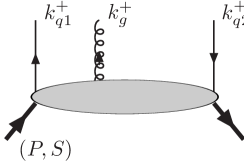
Figure 1: A vertex diagram representing twist-three quark-gluon correlation function in a proton. When the proton is polarized, the gluon field has a definite polarization.

Here, $|PS\rangle$ is the proton state with four-momentum $P^{\mu}$ and transverse-polarization vector $S^{\mu}=(0,0,\vec{S}_{\perp})$, $\bar{\psi}$, $\psi$ are the quark fields with color indices $i,j$ and Dirac indices $\rho,\sigma$, and $F^{+\alpha}_{a}$ is the gluon field strength tensor with octet color index $a$. $x_{1}=k_{q1}^{+}/P^{+}$, $x_{g}=k_{g}^{+}/P^{+}$, and $x_{2}=k_{q2}^{+}/P^{+}=x_{1}+x_{g}$ are the fractions of the proton’s light-cone momentum carried by the quarks and the gluon, where their momenta as shown in Fig. 1. Furthermore, ${\cal L}$ is the light-cone gauge link,

$${\cal L}(\xi_{2}^{-},\xi_{1}^{-})=P\exp\left(-ig\int^{\xi_{2}^{-}}_{\xi_{1}^{-}}d\xi^{-}A^{+}(\xi^{-})\right)\ ,$$ (2)

which makes the correlation operator gauge-invariant. Note that our sign convention for the strong coupling constant $g$ follows from $D^{\mu}\equiv\partial^{\mu}+igA^{\mu}$ for the covariant derivative. Also note that we have included a factor $g$ in the matrix element in Eq. (1), as compared to the definition in qiu . In the second line of (1), we have expanded the matrix in Dirac space, keeping only the leading, twist-three, term that contributes to the SSA in the Drell-Yan process, and neglecting contributions of yet higher twist. Here, $N_{C}=3$ is the number of colors, $C_{F}=(N_{C}^{2}-1)/2N_{C}=4/3$, and $T^{a}_{ij}$ denote the generators of the SU(3) color gauge group. $\epsilon^{\alpha\beta}_{\perp}$ is the 2-dimensional Levi-Civita tensor with $\epsilon^{12}_{\perp}=1$.

Inverting Eq. (1), we can express the correlation function $T_{F}(x_{1},x_{2})$ as follows:

$$T_{F}(x_{1},x_{2})=\int\frac{d\zeta^{-}d\eta^{-}}{4\pi}e^{ix_{1}P^{+}\eta^{-}}e^{i(x_{2}-x_{1})P^{+}\zeta^{-}}\epsilon_{\perp}^{\beta\alpha}S_{\perp\beta}\left\langle PS|\overline{\psi}(0)\gamma^{+}g{F^{+}}_{\alpha}(\zeta^{-})\psi(\eta^{-})|PS\right\rangle\ ,$$ (3)

where the sums over color and spin indices are now implicit and, for simplicity, we have omitted the gauge link which vanishes if one chooses to work in the light-cone gauge, $A^{+}=0$. Note that we have suppressed a renormalization scale dependence of $T_{F}$. Equation (3) provides the normalization for our calculations in the following sections. Because of parity and time-reversal invariance, the correlation function has the symmetry property qiu

$$T_{F}(x_{1},x_{2})=T_{F}(x_{2},x_{1})\ ,$$ (4)

which will be used later on to simplify our results.

III Single-Spin Drell-Yan Cross Section

We shall now calculate the single-transverse-spin dependent cross section for the Drell-Yan process, using the ETQS mechanism. We will first perform the calculation of the cross section at parton level. Convolution with the twist-three correlation function introduced in the last section and with the usual Feynman parton distributions for the unpolarized proton will then give the physical hadronic cross section. We shall limit ourselves to a situation where the dominant contributions come from the twist-three correlation function for a valence quark, and from an anti-quark or gluon of the unpolarized proton. In this way, we do not need to worry, for example, about other types of twist-three correlation functions, such as purely gluonic ones Ji:1992eu . In an actual experiment, such a situation may be realized when the lepton pair is produced in the forward direction of the polarized beam (at large rapidity), so that large momentum fractions in the polarized proton are probed.

As we discussed in the Introduction, we are primarily interested here in the Drell-Yan pair produced at large transverse momentum $q_{\perp}\sim Q$. For this to happen, a quark or gluon jet must be produced in the hard partonic process against which the Drell-Yan pair recoils. In the unpolarized case, to lowest order in perturbation theory, there are two partonic subprocesses of this kind: the Compton-type quark-gluon scattering $q+g\rightarrow\gamma^{*}+q$, and quark-antiquark annihilation $q+\bar{q}\rightarrow\gamma^{*}+g$. One therefore arrives at the following lowest-order (LO) expression of the unpolarized Drell-Yan cross section for producing a virtual photon of invariant mass $Q$, rapidity $y$, and transverse momentum $q_{\perp}$:

$$\frac{d^{4}\sigma}{dQ^{2}dyd^{2}q_{\perp}} = \sigma_{0}\frac{\alpha_{s}}{4\pi^{2}}\int\frac{dx}{x}\frac{dx^{\prime}}{x^{\prime}}\sum_{q}e_{q}^{2}\left[\hat{\sigma}_{q\bar{q}}(\hat{s},\hat{t},\hat{u})q(x)\bar{q}(x^{\prime})+\hat{\sigma}_{qg}(\hat{s},\hat{t},\hat{u})q(x)g(x^{\prime})\right]$$ (5)

$$\,\times\delta(\hat{s}+\hat{t}+\hat{u}-Q^{2})\ ,$$

where $\alpha_{s}$ is the strong coupling constant, and $\sigma_{0}=4\pi\alpha_{\rm em}^{2}/3N_{C}sQ^{2}$ with the electromagnetic coupling $\alpha_{\rm em}$ and the hadronic center-of-mass energy squared $s=(P+P^{\prime})^{2}$. Furthermore, $x$ and $x^{\prime}$ are the partons’ momentum fractions, and the partonic Mandelstam variables are defined as $\hat{s}=(xP+x^{\prime}P^{\prime})^{2}$, $\hat{t}=(xP-q_{\gamma^{*}})^{2}$, $\hat{u}=(x^{\prime}P^{\prime}-q_{\gamma^{*}})^{2}$ with the virtual photon momentum $q_{\gamma^{*}}$. Note that we have omitted the scale dependence of the parton distributions, as we will do throughout this paper.

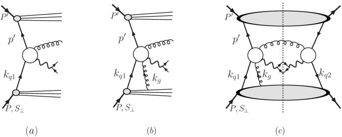
Figure 2: Drell-Yan scattering amplitudes via (a) $q+\bar{q}\rightarrow\gamma^{*}+g$ and (b) $q+\bar{q}+g\rightarrow\gamma^{*}+g$; (c) A typical diagram, from the interference of the amplitudes in (a) and (b), that gives a contribution to the SSA.

In order to have a non-vanishing single-transverse-spin asymmetry in a hadronic process, an interference of two amplitudes with different strong-interaction phases is required. When the underlying scattering mechanism is hard, as is the case for our Drell-Yan observable at large $Q$ and $q_{\perp}$, the difference in strong interaction phase may arise from the interference between a real part of the scattering amplitude in Fig. 2(a) and an imaginary part of the partonic scattering amplitude with an extra gluon in Fig. 2(b). The interference of these two amplitudes corresponds to the typical diagram contributing to the SSA shown in Fig. 2(c). The additional gluon of momentum $k_{g}$ from the polarized proton, which leads to the twist-three quark-gluon correlation function as shown in Fig. 1, can attach to any propagator of the hard part represented by a light circle in Fig. 2(b) or (c). The imaginary part of the amplitude with an extra gluon is provided by the pole of the parton propagator associated with the integration of the gluon momentum fraction $x_{g}=k_{g}^{+}/P^{+}$ qiu . In the previously considered cases of the SSAs in direct-photon or inclusive-hadron production, such poles only occur when the additional polarized gluon has a vanishing momentum, $x_{g}=0$ ($x_{1}=x_{2}$), while it is attached to an external on-shell parton qiu . These poles were referred to as “soft poles” luo ; guo . For example, if the polarized gluon attaches to the incoming unpolarized anti-quark, the on-shell propagation of the anti-quark line will generate such a soft and un-pinched gluonic pole. However, for the Drell-Yan process, there are two observed hard scales, $Q$ and $q_{\perp}$, because of the outgoing photon being off-shell, and there could be additional imaginary contributions associated with poles of propagators in the partonic scattering amplitude for which $x_{g}\neq 0$ ($x_{1}\neq x_{2}$). Such poles were called “hard poles” luo ; guo . In the calculations presented below, we shall consistently include both contributions, soft-pole and hard-pole ones. Compared to the unpolarized case in Eq. (5), we now find the following structure for the LO single-spin cross section:

$$\frac{d^{4}\Delta\sigma(S_{\perp})}{dQ^{2}dyd^{2}q_{\perp}} = \sigma_{0}\epsilon^{\alpha\beta}{S}_{\perp\alpha}q_{\perp\beta}\frac{\alpha_{s}}{2\pi^{2}}\int\frac{dx}{x}\frac{dx^{\prime}}{x^{\prime}}\sum_{q}e_{q}^{2}\left[\left(H_{q}^{s}+H_{q}^{h}\right)\bar{q}(x^{\prime})+\left(H_{g}^{s}+H_{g}^{h}\right)g(x^{\prime})\right]$$ (6)

$$\times\,\delta(\hat{s}+\hat{t}+\hat{u}-Q^{2})\ ,$$

where $H_{q,g}^{s}$ and $H_{q,g}^{h}$ are the soft- and hard-pole contributions for scattering off an unpolarized anti-quark or gluon, respectively. Each of these will be a function of the partonic Mandelstam variables, of $x$ and $x^{\prime}$, and of the twist-three quark-gluon correlation function $T_{F}(x_{1},x_{2})$. Note that $x$ is the same as in the unpolarized case, determined in terms of the external hadronic variables through the delta-function in (6). As will be described in detail below, $x_{1}$ and $x_{2}$ depend on $x$ and are fixed by the on-shell conditions set variously by the soft and hard poles, and by that for the unobserved final-state parton in the hard process.

In the following subsections, we will first discuss the generic features of the soft and hard poles, and then present their respective contributions to the single-transverse polarized cross sections for the quark-antiquark and quark-gluon scattering channels.

III.1 Generic Structure of Soft and Hard Poles

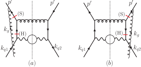
Figure 3: A typical Feynman diagram (a) and its complex conjugate (b) contributing to the single-spin asymmetry for the Drell-Yan process through the quark-antiquark scattering channel, containing both soft-pole “(S)” and hard-pole “(H)” contributions. The bars indicate the places where a pole arises and generates a strong interaction phase.

We will take the diagrams shown in Fig. 3 as examples of how the soft and hard poles arise. Let $p^{\prime}$ denote the momentum of the incident anti-quark, $k_{q1}$ that of the initial quark to the left of the cut, $k_{q2}$ that on the right, and $k_{g}=k_{q2}-k_{q1}$ the momentum of the polarized gluon attaching to the hard part. This attachment may happen on the left side of the cut, as shown in Fig 3(a), or on the right side as in 3(b). In order to analyze the pole structure in the scattering amplitudes, it is convenient to consider only the dominant components of the relevant momenta. For example, $p^{\prime}$ may be chosen to only have a light-cone “minus” component, while $k_{q1}$ and $k_{q2}$ are then dominated by their plus components. When the polarized gluon attaches to the left side of the cut in Fig. 3(a), we find that the on-shell condition for the gluon radiated into the final state fixes $k_{q2}^{+}$ (or, equivalently, $x_{2}$) to be $x_{2}\approx x$, while $k_{q1}^{+}$ ($x_{1}$) is determined by the (soft- or hard-) pole condition. On the other hand, the momentum flow in Fig. 3(b) is opposite: $x_{1}$ is determined by the on-shell condition for the outgoing gluon, and $x_{2}$ by the pole of a propagator.

In Fig. 3, we have denoted the poles by bars, and introduced the labels $(S)$ and $(H)$ for the soft and hard poles, respectively. A soft pole arises in Fig. 3(a) on the anti-quark line carrying momentum $p^{\prime}+k_{g}$, because we have

$$\frac{1}{(p^{\prime}+k_{g})^{2}+i\epsilon}=\frac{1}{2p^{{}^{\prime}-}P^{+}}\frac{1}{x_{g}+i\epsilon}\ ,$$ (7)

which provides a phase proportional to $\delta(x_{g})=\delta(x_{1}-x_{2})$. Therefore, the quark-gluon correlation function $T_{F}(x_{1},x_{2})$ will be probed when both of its arguments are identical. After combining with the on-shell condition for the unobserved final-state gluon, one finds in fact that the contribution enters with $T_{F}(x,x)$ . Similarly, the soft pole in Fig. 3(b) will arise through

$$\frac{1}{(p^{\prime}-k_{g})^{2}-i\epsilon}=\frac{1}{2p^{{}^{\prime}-}P^{+}}\frac{1}{-x_{g}-i\epsilon}\ ,$$ (8)

so that it enters with opposite sign compared to that of Fig. 3(a), but with otherwise the same quark-gluon correlation function. Therefore, the contributions by the two poles in Eqs. (7),(8) may be combined.

Next, we turn to the hard pole in Fig. 3(a). It occurs when the quark propagator carrying momentum $k_{q1}-q_{\gamma^{*}}$ goes on mass-shell. The propagator reads

$$\frac{1}{(k_{q1}-q_{\gamma^{*}})^{2}+i\epsilon}\approx\frac{1}{-2k_{q1}^{+}q_{\gamma^{*}}^{-}+Q^{2}+i\epsilon}\ ,$$ (9)

where we have neglected the transverse momentum $k_{q1\perp}$. It is easy to see that this propagator has a pole at $k_{q1}^{+}=xP^{+}{Q^{2}}/{(Q^{2}-\hat{t})}$, corresponding to $x_{g}=\bar{x}_{g}$, where

$$\bar{x}_{g}\equiv-x\hat{t}/(Q^{2}-\hat{t})\ .$$ (10)

Because $\hat{t}=(xP-q_{\gamma^{*}})^{2}<0$, this pole is not forbidden kinematically. Furthermore, $x_{g}>0$, which is the reason why we refer to the pole as “hard”. After taking the pole, we find $x_{1}=x-\bar{x}_{g}$. Using the on-shell condition for the outgoing gluon, the associated twist-three correlation eventually is $T_{F}(x-\bar{x}_{g},x)$, different from that for the soft-pole contributions. Likewise, the hard pole in Fig. 3(b) arises from the propagator

$$\frac{1}{(k_{q2}-q_{\gamma^{*}})^{2}-i\epsilon}\approx\frac{1}{-2k_{q2}^{+}q_{\gamma^{*}}^{-}+Q^{2}-i\epsilon}\ ,$$ (11)

and is at $k_{q2}^{+}=xP^{+}{Q^{2}}/{(Q^{2}-\hat{t})}$, corresponding to $x_{g}=-\bar{x}_{g}=x\hat{t}/(Q^{2}-\hat{t})<0$. The associated twist-three quark-gluon correlation function becomes $T_{F}(x,x-\bar{x}_{g})$. Because of the symmetry property (4) of the function, we have $T_{F}(x,x-\bar{x}_{g})=T_{F}(x-\bar{x}_{g},x)$, and we may again combine the contributions from the two sides of the cut in the diagram.

From kinematics, we find that hard poles only arise from $t$-channel propagators, and only on the side of the diagram that contains the additional gluon from the polarized proton. For each diagram, we have to include all contributions by the soft and hard poles, in order to obtain the complete result. Although we will calculate their contributions separately, the soft and hard poles do overlap in some kinematical regions, for example, when the transverse momentum $q_{\perp}$ is much smaller than $Q$. We will discuss this more in Sec. IV.

III.2 Soft-Pole Contributions

In this subsection, we calculate the soft gluonic pole contributions to the single-transversely-polarized Drell-Yan cross section in the LO quark-antiquark and quark-gluon scattering channels. The calculation is rather similar to that performed for direct-photon production in Ref. qiu , except for the fact that the photon is now virtual.

III.2.1 Soft Poles in Quark-Antiquark Scattering

We start by recalling the unpolarized hard-scattering function for the subprocess $q+\bar{q}\rightarrow\gamma^{*}+g$, appearing in Eq. (5):

$$\hat{\sigma}_{q\bar{q}}(\hat{s},\hat{t},\hat{u})=2C_{F}\left(\frac{\hat{u}}{\hat{t}}+\frac{\hat{t}}{\hat{u}}+\frac{2Q^{2}\hat{s}}{\hat{u}\hat{t}}\right)\ ,$$ (12)

where $C_{F}$ is the color-factor and the partonic Mandelstam variables are as defined after Eq. (5) at the beginning of this section.

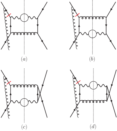
Figure 4: Feynman diagrams for the soft-pole contributions to the single-transverse-spin asymmetry through the quark-antiquark scattering channel. The bars indicate the propagators yielding poles.

For the single-spin cross section in this channel, there are eight partonic diagrams possessing soft poles. Four of them are shown in Fig. 4, and the other four are obtained by attaching the polarized gluon in the same way on the right side of the cut. Other attachments of the polarized gluon either do not give a soft pole, or simply cancel after summing over cuts.

It is useful to recapitulate some of the key steps in calculating the diagrams in Fig. 4 qiu . We perform our calculations using a covariant gauge. The polarized gluon is associated with a gauge potential $A^{\mu}$, and one of the leading contributions comes from its component $A^{+}$. The gluon’s momentum is dominated by $x_{g}P+k_{g\perp}$, where $x_{g}$ is the longitudinal momentum fraction with respect to the polarized proton. The transverse momentum $k_{g\perp}$ flows through the perturbative diagram and returns to the polarized proton through the quark lines. The contribution to the single-transverse-spin asymmetry arises from terms linear in $k_{g\perp}$ which, when combined with $A^{+}$, yield $\partial^{\perp}A^{+}$, a part of the gauge field strength tensor $F^{\perp+}$. In order to compute this contribution, we expand the partonic scattering amplitudes in terms of $k_{g\perp}$ up to the linear term. One important contribution to the $k_{g\perp}$ expansion comes from the on-shell condition for the outgoing unobserved quark, whose momentum depends on $k_{g\perp}$. As was shown in qiu , this leads to a term involving the derivative of the correlation function $T_{F}$. Apart from this contribution, the $k_{g\perp}$ expansion of the propagators and the Dirac traces yields a term proportional to the correlation function itself. This is the so-called non-derivative term.

The sum of the soft-pole contributions by the diagrams in Fig. 4 and their “mirror images” gives the function $H_{q}^{s}$ in Eq. (6). We find:

$$H_{q}^{s} = \left[x\frac{\partial}{\partial x}T_{F}(x,x)\right]\frac{D^{s}_{q\bar{q}}}{-\hat{u}}+T_{F}(x,x)\frac{N^{s}_{q\bar{q}}}{-\hat{u}}\ ,$$ (13)

where the hard coefficients $D^{s}_{q\bar{q}}$ and $N^{s}_{q\bar{q}}$ are

$$D^{s}_{q\bar{q}} = \frac{1}{2(N_{C}^{2}-1)}\,\hat{\sigma}_{q\bar{q}}(\hat{s},\hat{t},\hat{u})\ ,$$

$$N^{s}_{q\bar{q}} = \frac{1}{2N_{C}}\frac{1}{\hat{t}^{2}\hat{u}}\left[Q^{2}(\hat{u}^{2}-\hat{t}^{2})+2Q^{2}\hat{s}(Q^{2}-2\hat{t})-(\hat{u}^{2}+\hat{t}^{2})\hat{t}\right]\ ,$$

where $\hat{\sigma}_{q\bar{q}}$ in the first line is the unpolarized hard-scattering function given in Eq. (12), implying that the hard-scattering function for the derivative term differs from the unpolarized one only by the color factor Ratcliffe . In the real-photon limit, $Q^{2}\to 0$, we obtain the annihilation contribution to the direct-photon single-spin cross section.

III.2.2 Soft Poles in Quark-Gluon Scattering

Again we start by giving the hard-scattering function for the unpolarized case:

$$\hat{\sigma}_{qg}(\hat{s},\hat{t},\hat{u})=2T_{R}\left(\frac{\hat{s}}{-\hat{t}}+\frac{-\hat{t}}{\hat{s}}-\frac{2Q^{2}\hat{u}}{\hat{s}\hat{t}}\right)\,,$$ (14)

where $T_{R}=1/2$.

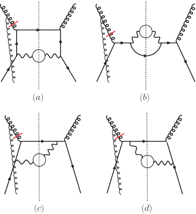
Figure 5: Feynman diagrams for soft-pole contributions to the single-transverse-spin asymmetry through quark-gluon scattering.

Feynman diagrams for the soft-pole contributions to the single-transverse-spin asymmetry are shown in Fig. 5, where again the diagrams for the attachments of the polarized gluon to the incident gluon on the right side of cut have been omitted. Following the same calculational procedure as outlined earlier, the soft-pole contributions for the quark-gluon channel are:

$$H_{g}^{s} = \left[x\frac{\partial}{\partial x}T_{F}(x,x)\right]\frac{D^{s}_{qg}}{-\hat{u}}+T_{F}(x,x)\frac{N^{s}_{qg}}{-\hat{u}}\ ,$$ (15)

where the first term is the derivative term and the second the non-derivative one, with

$$D^{s}_{qg} = -\frac{N_{C}^{2}}{2(N_{C}^{2}-1)}\,\hat{\sigma}_{qg}(\hat{s},\hat{t},\hat{u})\ ,$$

$$N^{s}_{qg} = \frac{N_{C}^{2}}{2(N_{C}^{2}-1)}\frac{1}{\hat{t}^{2}\hat{s}}\left[Q^{2}(\hat{s}^{2}-\hat{t}^{2})+2Q^{2}\hat{u}(Q^{2}-2\hat{t})-(\hat{s}^{2}+\hat{t}^{2})\hat{t}\right]\ .$$

We note that apart from the color factor, the hard coefficients $D^{s}_{qg}$ and $N^{s}_{qg}$ for the quark-gluon scattering channel can be obtained from those for the quark-antiquark channel by “crossing” $\hat{s}\leftrightarrow\hat{u}$. In the limit $Q^{2}=0$, we obtain the direct-photon cross section, which was calculated previously in qiu . We agree with the derivative term found there, but find a difference for the non-derivative one.

III.3 Hard-Pole Contributions

In this subsection, we will calculate the hard-pole contributions to the single-spin cross section. The calculational procedure is similar to that for the soft-pole contributions in the previous subsection. We will again discuss the quark-antiquark and quark-gluon channels separately.

III.3.1 Hard Poles in Quark-Antiquark Scattering

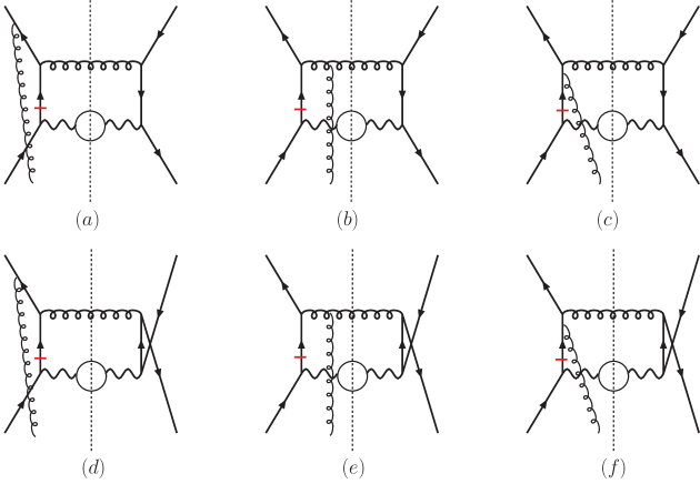
Figure 6: Hard-pole contributions in the quark-antiquark scattering channel. The bar indicates the propagator that produces the pole.

In Fig. 6 we show the hard-pole diagrams for the quark-antiquark scattering channel, again omitting the “mirror” diagrams. As discussed in subsection III.A, only $t$-channel propagators give a hard pole. In the quark-antiquark scattering channel, there are only two basic diagrams containing a $t$-channel propagator, shown in Figs. 6(a) and (d). However, because of gauge invariance, we need to allow all possible gluon attachments in these diagrams. We thus have attachments to the initial antiquark line, to the outgoing gluon line and to the $t$-channel quark propagator, as shown in the figure. Therefore, including the diagrams with gluon attachments on the right side of the cut, there will be a total of twelve diagrams containing hard poles in the quark-antiquark scattering channel. We may group their contributions into two color structures: ${\rm Tr}(T^{a}T^{b}T^{a}T^{b})$ for diagrams (a) and (d), and ${\rm Tr}(T^{a}T^{a}T^{b}T^{b})$ for diagrams (c) and (f). The first color factor is the same as for the soft gluonic pole diagrams. The color traces for diagrams (b) and (e) can be decomposed into these two color structures, and combined with (a,d) and (c,f), using the fact that $if_{abc}T^{c}=T^{a}T^{b}-T^{b}T^{a}$.

The expansion in $k_{g\perp}$ for the hard-pole contributions is somewhat more complicated than for the soft-pole ones, because the position of the hard pole itself depends on $k_{g\perp}$. As an example we consider the diagram in Fig. 6(a), for which a hard pole arises from the propagator

$$\frac{1}{(k_{q1}-q_{\gamma^{*}})^{2}+i\epsilon}=\frac{1}{-2k_{q1}^{+}q_{\gamma^{*}}^{-}+Q^{2}-2k_{q1\perp}\cdot q_{\gamma^{*}\perp}+i\epsilon}\ ,$$ (16)

where we have kept the full dependence on the transverse momentum. In the $k_{g\perp}$-expansion, the $k_{q1\perp}$ term in the above denominator will make a contribution to the term linear in $k_{g\perp}$, because $k_{g\perp}=k_{q2\perp}-k_{q1\perp}$. This will lead to a derivative term (of $T_{F}$), similar to the double-pole contributions found in qiu for the SSA in single-inclusive hadron production. In the calculation of this derivative term, we may set $k_{g\perp}=0$ everywhere else in the scattering amplitude. Because all the propagators with hard poles in Fig. 6 are $t$-channels and hence have the same momentum, namely $k_{q1}-q_{\gamma^{*}}$, the expansion will be the same for all diagrams, and we may add their contributions. After summing over all the diagrams, we find that the total derivative contribution vanishes. More precisely, the derivative contributions from the hard poles in diagrams (a), (b), (d) and (e) (which all contain the color structure ${\rm Tr}(T^{a}T^{b}T^{a}T^{b})$) cancel each other, and the same happens for the contributions by diagrams (b), (c), (e) and (f) (which enter with ${\rm Tr}(T^{a}T^{a}T^{b}T^{b})$).

The expansion of the delta function associated with the on-shell condition for the outgoing unobserved gluon ($(k_{q2}+p^{\prime}-q_{\gamma^{*}})^{2}=0$) also contributes to the derivative term for each individual diagram. However, after summing over all diagrams, again the net derivative contribution vanishes. In summary, we do not have any derivative contributions originating from the hard poles.

For the non-derivative contributions, we need to do an expansion of the numerator (for example, the Dirac trace) and of the other propagators in the squared amplitude. Apart from that, the derivative terms just discussed will make contributions to the non-derivative pieces. Our way of dealing with the non-derivative contributions is to first evaluate the scattering amplitudes with their full dependence on $k_{g\perp}$, and then to use the on-shell condition for the outgoing unobserved gluon and the hard-pole condition, in order to fix the light-cone momentum fractions of the quarks including their dependence on $k_{g\perp}$. For example, the on-shell condition for $k_{q2}+p^{\prime}-k_{\gamma^{*}}$ in Fig. 6(a) determines the value for $k_{q2}^{+}$:

$$k_{q2}^{+}=xP^{+}\left(1-\frac{2k_{q2\perp}.q_{\perp}}{\hat{u}}\right)\ .$$ (17)

Similarly, the hard-pole condition $(k_{q1}-k_{\gamma^{*}})^{2}=0$ fixes the value for $k_{q1}^{+}$ as

$$k_{q1}^{+}=xP^{+}\frac{Q^{2}}{Q^{2}-\hat{t}}\left(1-\frac{2k_{q1\perp}.q_{\perp}}{Q^{2}}\right)\ .$$ (18)

From the above equations, we see that both $k_{q1}^{+}$ and $k_{q2}^{+}$ depend on $k_{g\perp}$, so that their expansion will contribute to a non-derivative term.

Summing over all the contributions by the diagrams in Fig. 6 and their “mirror images”, we obtain the final result for the non-derivative hard-pole contribution for the quark-antiquark channel:

$$H_{q}^{h}=T_{F}(x-\bar{x}_{g},x)\times\frac{(Q^{2}-\hat{t})^{3}+Q^{2}\hat{s}^{2}}{\hat{t}^{2}\hat{u}^{2}}\left[\frac{1}{2N_{C}}+C_{F}\frac{\hat{s}}{\hat{s}+\hat{u}}\right]\ ,$$ (19)

where as before $\bar{x}_{g}=-x\hat{t}/(Q^{2}-\hat{t})$ is different from zero, reflecting the hard-pole nature of the contribution. The two color factors in the above equation are associated with the two independent color structures discussed earlier, the first one coming from ${\rm Tr}(T^{a}T^{b}T^{a}T^{b})$ and the second one from ${\rm Tr}(T^{a}T^{a}T^{b}T^{b})$.

III.3.2 Hard Poles in the Quark-Gluon Channel

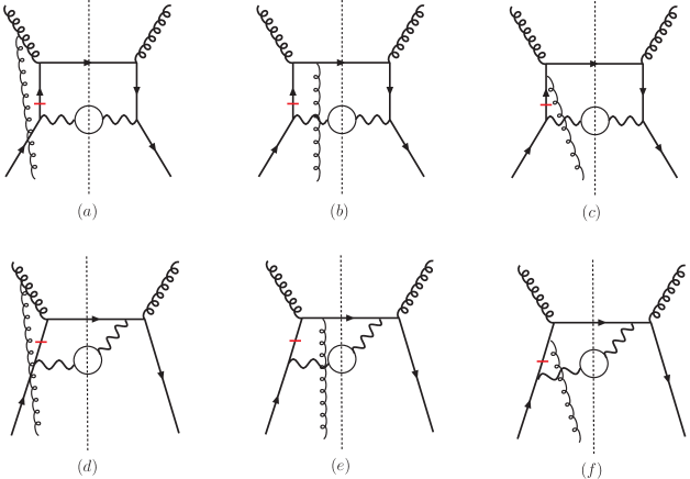
Figure 7: Hard pole contributions in the quark-gluon scattering channel. The bar indicates the propagator that produces the pole.

By a similar procedure, we calculate the hard-pole contributions for the quark-gluon scattering channel. In Fig. 7, we show the relevant diagrams. Following the same arguments as given for the quark-antiquark scattering channel, only $t$-channel diagrams contribute to the hard poles, and their total contribution is

$$H_{g}^{h}=T_{F}(x-\bar{x}_{g},x)\times\frac{(Q^{2}-\hat{t})^{3}+Q^{2}\hat{u}^{2}}{-\hat{u}\hat{t}^{2}\hat{s}}\left[\frac{-N_{C}^{2}}{2(N_{C}^{2}-1)}+T_{R}\frac{\hat{s}}{\hat{s}+\hat{u}}\right]\ .$$ (20)

Again, there are no derivative terms, and the hard coefficient for the non-derivative term is related to that for quark-antiquark scattering given above by $\hat{s}\leftrightarrow\hat{u}$ crossing. As for the $q\bar{q}$ case, there are two contributing color structures, one associated with $if_{abc}{\rm Tr}(T^{a}T^{b}T^{c})$ (for diagrams Fig. 7(a), (b), (d), and (e)), and one with ${\rm Tr}(T^{a}T^{a}T^{b}T^{b})$ (for diagrams Fig. 7(c), (b), (f), and (e)).

IV Low Transverse Momentum Limit

Having calculated the full LO single-spin cross section for the Drell-Yan process at large $q_{\perp}$ within the ETQS approach, we are now in the position to investigate the limit $\Lambda_{\rm QCD}\ll q_{\perp}\ll Q$, trying to make contact with the approach based on transverse-momentum dependent factorization. To this end, we expand the formulas given in the preceding section for small $q_{\perp}/Q$, extracting their leading contributions.

The partonic Mandelstam variables may be written as

$$\hat{s} = \frac{q_{\perp}^{2}}{(1-\xi_{1})(1-\xi_{2})}\ ,$$ (21)

$$\hat{t} = -\frac{q_{\perp}^{2}}{1-\xi_{2}}\ ,$$ (22)

$$\hat{u} = -\frac{q_{\perp}^{2}}{1-\xi_{1}}\ ,$$ (23)

where $\xi_{1}=z_{1}/x$ and $\xi_{2}=z_{2}/x^{\prime}$, with $z_{1}=Q/\sqrt{s}e^{y}$ and $z_{2}=Q/\sqrt{s}e^{-y}$. The phase-space delta-function for the on-shell condition for the outgoing parton takes the form meng

$$\delta(\hat{s}+\hat{t}+\hat{u}-Q^{2}) = \delta(\hat{s}(1-\xi_{1})(1-\xi_{2})-q_{\perp}^{2})$$ (24)

$$= \frac{1}{\hat{s}}\left[\frac{\delta(\xi_{2}-1)}{(1-\xi_{1})_{+}}+\frac{\delta(\xi_{1}-1)}{(1-\xi_{2})_{+}}+\delta(\xi_{1}-1)\delta(\xi_{2}-1)\ln\frac{Q^{2}}{q_{\perp}^{2}}\right]\ ,$$

where the “plus”-prescription is defined in the standard way through

$$\int_{x}^{1}dz\frac{f(z)}{(1-z)_{+}}=\int_{x}^{1}dz\frac{f(z)-f(1)}{1-z}+f(1)\ln(1-x)\ ,$$ (25)

for any suitably regular function $f$.

After applying Eq. (24) to the results presented in the previous subsections, we find for the small-$q_{\perp}$ behavior of the unpolarized cross section for $q+\bar{q}\to\gamma^{*}g$:

$$\frac{d^{4}\sigma^{q\bar{q}\to\gamma^{*}g}}{dQ^{2}dyd^{2}q_{\perp}} = \sigma_{0}\frac{\alpha_{s}}{2\pi^{2}}C_{F}\frac{1}{q_{\perp}^{2}}\int\frac{dx}{x}\frac{dx^{\prime}}{x^{\prime}}\sum_{q}e_{q}^{2}q(x)\bar{q}(x^{\prime})\left[\frac{1+\xi_{1}^{2}}{(1-\xi_{1})_{+}}\delta(\xi_{2}-1)\right.$$ (26)

$$\left.+\frac{1+\xi_{2}^{2}}{(1-\xi_{2})_{+}}\delta(\xi_{1}-1)+2\delta(\xi_{1}-1)\delta(\xi_{2}-1)\ln\frac{Q^{2}}{q_{\perp}^{2}}\right]\ .$$

For $q+g\to\gamma^{*}q$ scattering, we obtain

$$\frac{d^{4}\sigma^{qg\to\gamma^{*}q}}{dQ^{2}dyd^{2}q_{\perp}} = \sigma_{0}\frac{\alpha_{s}}{4\pi^{2}}\frac{1}{q_{\perp}^{2}}\int\frac{dx}{x}\frac{dx^{\prime}}{x^{\prime}}\sum_{q}e_{q}^{2}q(x)g(x^{\prime})\delta(1-\xi_{1})\left[\xi_{2}^{2}+(1-\xi_{2})^{2}\right]\ .$$ (27)

These results are well-known in the literature ColSopSte85 .

We now make similar expansions for the single-spin cross sections. As we anticipated, at low transverse momentum, the soft- and hard-pole contributions overlap: at $q_{\perp}=0$, the twist-three quark-gluon correlation function associated with the hard-pole contributions, $T_{F}(x-\bar{x}_{g},x)$, becomes $T_{F}(x-x(1-\xi_{1})/\xi_{2},x)$, which at $\xi_{1}=1$ is identical to the correlation function $T_{F}(x,x)$ that accompanies the soft poles.

For the $q\bar{q}$ channel, we find:

$$\frac{d^{4}\Delta\sigma^{q\bar{q}\to\gamma^{*}g}(S_{\perp})}{dQ^{2}dyd^{2}q_{\perp}} = \sigma_{0}\,\epsilon^{\alpha\beta}{S}_{\perp\alpha}\,\frac{q_{\perp\beta}}{(q_{\perp}^{2})^{2}}\,\frac{\alpha_{s}}{2\pi^{2}}\int\frac{dx}{x}\frac{dx^{\prime}}{x^{\prime}}\bar{q}(x^{\prime})\left\{\delta(\xi_{2}-1)A+\delta(\xi_{1}-1)B\right\}\,,$$ (28)

where

$$A = \frac{1}{2N_{C}}\left\{\left[x\frac{\partial}{\partial x}T_{F}(x,x)\right](1+\xi_{1}^{2})+T_{F}(x,x-\widehat{x}_{g})\frac{1+\xi_{1}}{(1-\xi_{1})_{+}}\right.$$ (29)

$$\left.+T_{F}(x,x)\frac{(1-\xi_{1})^{2}(2\xi_{1}+1)-2}{(1-\xi_{1})_{+}}\right\}+C_{F}T_{F}(x,x-\widehat{x}_{g})\frac{1+\xi_{1}}{(1-\xi_{1})_{+}}\ ,$$

$$B = C_{F}T_{F}(x,x)\left[\frac{1+\xi_{2}^{2}}{(1-\xi_{2})_{+}}+2\delta(\xi_{2}-1)\ln\frac{Q^{2}}{q_{\perp}^{2}}\right]\ ,$$ (30)

with $\widehat{x}_{g}\equiv(1-\xi_{1})x$.

For the $qg$ channel, the contribution involving the derivative $dT_{F}(x,x)/dx$ turns out to be of higher order in $q_{\perp}/Q$. The full non-derivative term becomes

$$\frac{d^{4}\Delta\sigma^{qg\to\gamma^{*}q}(S_{\perp})}{dQ^{2}dyd^{2}q_{\perp}} = \sigma_{0}\,\epsilon^{\alpha\beta}{S}_{\perp\alpha}\,\frac{q_{\perp\beta}}{(q_{\perp}^{2})^{2}}\sum_{q}e_{q}^{2}T_{F}(z_{1},z_{1})$$ (31)

$$\times\frac{\alpha_{s}}{2\pi^{2}}T_{R}\int\frac{dx_{2}}{x_{2}}g(x_{2})\left[\xi_{2}^{2}+(1-\xi_{2})^{2}\right].$$

In the following section, we will reproduce the above results from a QCD factorization in terms of transverse-momentum-dependent parton distributions.

V Transverse-momentum-dependent QCD Factorization

When $q_{\perp}\ll Q$, the Drell-Yan cross section in leading order in $q_{\perp}/Q$ may be calculated from a QCD factorization theorem involving transverse-momentum-dependent (TMD) parton distributions ColSopSte85 ; JiMaYu04 . Therefore, one expects that the results given in the previous section can be reproduced by this alternative approach. Indeed, for the unpolarized cross section this is well established ColSopSte85 ; Laenen:2000ij .

V.1 Transverse-Momentum-Dependent Parton Distributions

Transverse-momentum-dependent parton distributions were first introduced by Collins and Soper ColSop81 . They provide more information about the structure of the nucleon than is contained in the usual Feynman parton distributions. Based on rigorous factorization theorems ColSop81 ; JiMaYu04 ; ColMet04 , these distributions may be extracted from various processes that are characterized by a large momentum scale and a much smaller, measured, transverse momentum, such as semi-inclusive DIS and the Drell-Yan process. In this paper, we follow a definition of the TMD distributions in Feynman gauge with explicit gauge links Col02 . We avoid the axial gauge because of the complications presented by additional gauge links at space-time infinity BelJiYua02 .

The TMD quark distributions of a polarized proton may be defined through the following matrix:

$${\cal M}^{\alpha\beta} = P^{+}\int\frac{d\xi^{-}}{2\pi}e^{-ix\xi^{-}P^{+}}\int\frac{d^{2}b_{\perp}}{(2\pi)^{2}}e^{i\vec{b}_{\perp}\cdot\vec{k}_{\perp}}\,\left\langle PS\left|\overline{\mit\Psi}_{v}^{\beta}(\xi^{-},0,\vec{b}_{\perp}){\mit\Psi}_{v}^{\alpha}(0)\right|PS\right\rangle\ ,$$ (32)

where the vector $P=(P^{+},0^{-},0_{\perp})$ is along the momentum direction of the proton, $S$ is the polarization vector, and ${\mit\Psi}_{v}(\xi)$ is defined as

$${\mit\Psi}_{v}(\xi)\equiv{\cal L}_{v}(-\infty;\xi)\psi(\xi)\ ,$$ (33)

with the gauge link

$${\cal L}_{v}(-\infty;\xi)\equiv\exp\left(-ig\int^{-\infty}_{0}d\lambda\,v\cdot A(\lambda v+\xi)\right)\ .$$ (34)

This gauge link goes to $-\infty$, indicating that we adopt the definition for the TMD quark distributions for the Drell-Yan process BroHwaSch02 ; Col02 ; BelJiYua02 . In a coordinate system where $P^{+}\gg P^{-}$, the vector $v$ in the above equations is taken to have $v^{-}\gg v^{+},v_{\perp}=0$, with a nonzero $v^{+}$ component that regulates the light-cone singularities. The leading-power expansion of the density matrix ${\cal M}$ contains eight quark distributions MulTanBoe . Here, we are only interested in the TMD distributions for (un)polarized quarks and antiquarks in the polarized proton, in particular in the Sivers functions. The physics of the Sivers functions may be viewed as follows. Consider a transversely polarized proton with large momentum $P$. The distribution of quarks with longitudinal and transverse momenta $xP$ and $\vec{k}_{\perp}$ can have a dependence on the orientation of $\vec{k}_{\perp}$ relative to the proton’s polarization vector $\vec{S}_{\perp}$. Keeping only the unpolarized quark distribution and the Sivers function, we have the following expansion for the matrix ${\cal M}$:

$${\cal M}=\frac{1}{2}\left[q(x,k_{\perp})\gamma_{\mu}P^{\mu}+\frac{1}{M_{P}}\,q_{T}(x,k_{\perp})\,\epsilon_{\mu\nu\alpha\beta}\gamma^{\mu}P^{\nu}k^{\alpha}S^{\beta}+\ldots\right]$$ (35)

where $q(x,k_{\perp})$ is the TMD distribution in an unpolarized proton, $q_{T}(x,k_{\perp})$ is the Sivers function, and $M_{P}$ is a hadron mass, used to normalize $q(x,k_{\perp})$ and $q_{T}(x,k_{\perp})$ to the same mass dimension.

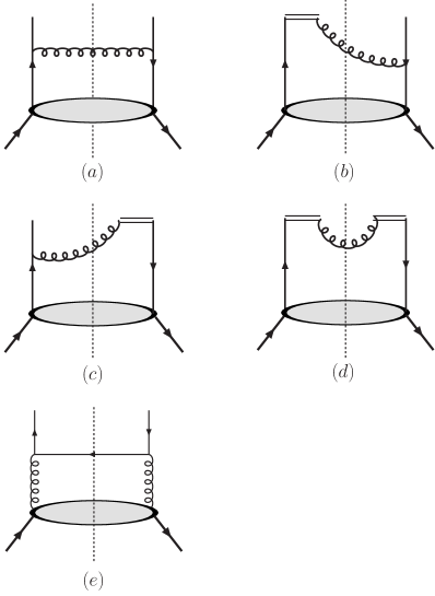
Figure 8: Feynman diagrams contributing to the spin-independent quark distribution at large transverse momentum $k_{\perp}\gg\Lambda_{\rm QCD}$, arising from the integrated quark (a-d) and gluon (e) distributions. Double lines denote Eikonal lines.

When the transverse momentum $k_{\perp}$ is low, say, of order of $\Lambda_{\rm QCD}$, the TMD parton distributions are entirely non-perturbative objects. Thus, the only way of treating them is to parameterize them in a suitable way, and to fit them to data. However, for much larger transverse momentum, $k_{\perp}\gg\Lambda_{\rm QCD}$, the $k_{\perp}$-dependence of the TMD parton distributions can be calculated within perturbative QCD, because a hard gluon has to be radiated in order to generate the $k_{\perp}$. Through the pQCD calculation, the TMD parton distributions may be related to the $k_{\perp}$-integrated parton distributions (or, in case of the Sivers functions, to the twist-three quark-gluon correlation function, as we shall show below), multiplied by calculable hard coefficients. For example, the TMD quark distribution for an unpolarized proton at large $k_{\perp}$ will receive contributions from the $k_{\perp}$-integrated quark and gluon distributions. The relevant Feynman diagrams are shown in Fig. 8, and the results for the first-order term are (see, for example, JiMaYu04 ; JiMaYu05 ):

$$q(z,k_{\perp}) = \frac{\alpha_{s}}{2\pi^{2}}\frac{1}{\vec{k}_{\perp}^{2}}C_{F}\int\frac{dx}{x}q(x)\left[\frac{1+\xi^{2}}{(1-\xi)_{+}}+\delta(\xi-1)\left(\ln\frac{z^{2}\zeta^{2}}{\vec{k}_{\perp}^{2}}-1\right)\right]$$ (36)

$$+\frac{\alpha_{s}}{2\pi^{2}}\frac{1}{\vec{k}_{\perp}^{2}}T_{R}\int\frac{dx}{x}g(x)\left[\xi^{2}+(1-\xi)^{2}\right]\ ,$$

where $q(x)$ and $g(x)$ are the integrated quark and gluon distributions, $\xi=z/x$, and $\zeta^{2}=(2v\cdot P)^{2}/v^{2}$. A similar expression is obtained for the anti-quark TMD distribution. We note that upon including virtual corrections, we would find that the term $1/\vec{k}_{\perp}^{2}$ would be converted to a term $1/(\vec{k}_{\perp}^{2})_{+}$, and similarly for the logarithmic term. This “plus”-prescription would make the distribution integrable at low $k_{\perp}$; for details, see for example aegm .

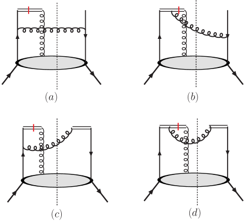
Figure 9: Feynman diagrams contributing to the Sivers functions at a large transverse momentum $k_{\perp}\gg\Lambda_{\rm QCD}$, arising from the twist-three quark-gluon correlation in Fig. 1: soft-pole contributions.

In the same spirit, the Sivers function at large $k_{\perp}$ can also be calculated perturbatively. Because it is (naively) time-reversal-odd, the only contribution comes from the twist-three quark-gluon correlation, with the phase provided by the hard part. This is very similar to the case of the single transverse-spin dependent Drell-Yan cross section calculated in Sec. III. Also in the present calculation, we will have soft-pole and hard-pole contributions, shown in Figs. 9 and 10, respectively. Carrying out the calculations accordingly, we find for the soft-pole contributions:

$$q_{T}(z,k_{\perp})|_{\rm soft-pole} = \frac{\alpha_{s}}{4\pi^{2}}\frac{2M_{P}}{(\vec{k}_{\perp}^{2})^{2}}\frac{1}{2N_{C}}\int\frac{dx}{x}\left\{\left[x\frac{\partial}{\partial x^{\prime}}T_{F}(x,x)\right]\left(1+\xi^{2}\right)\right.$$ (37)

$$+ \left.T_{F}(x,x)\left[\frac{(1-\xi)^{2}(2\xi+1)-2}{(1-\xi)_{+}}-\delta(\xi-1)\left(\ln\frac{z^{2}\zeta^{2}}{k_{\perp}^{2}}-1\right)\right]\right\},$$

where the $1/(k_{\perp}^{2})^{2}$ behavior also follows from power counting, and where $\xi$ and $\zeta$ as defined above after Eq. (36). We note that our choice of the direction of the gauge link in Eq. (34) is crucial since it determines the sign of the Sivers function BroHwaSch02 ; Col02 ; BelJiYua02 . Only with the correct choice (in this case, to $-\infty$) can the factorization work out eventually. In case of semi-inclusive DIS a different choice is necessary, and the resulting Sivers function will have opposite sign.

The hard-pole contributions can be calculated similarly, and we find

$$q_{T}(z,k_{\perp})|_{\rm hard-pole} = \frac{\alpha_{s}}{4\pi^{2}}\frac{2M_{P}}{(\vec{k}_{\perp}^{2})^{2}}\left[C_{F}+\frac{1}{2N_{C}}\right]\int\frac{dx}{x}T_{F}(x,x-\widehat{x}_{g})$$ (38)

$$\times\left[\frac{1+\xi}{(1-\xi)_{+}}+\delta(\xi-1)\left(\ln\frac{z^{2}\zeta^{2}}{k_{\perp}^{2}}-1\right)\right],$$

where $\widehat{x}_{g}=(1-\xi)x$. Adding the above soft-pole and hard-pole contributions, we obtain the final result for the Sivers function at large $k_{\perp}$:

$$q_{T}(z_{1},k_{\perp}) = \frac{\alpha_{s}}{4\pi^{2}}\frac{2M_{P}}{(\vec{k}_{\perp}^{2})^{2}}\int\frac{dx}{x}\left\{A+C_{F}T_{F}(x,x)\delta(\xi_{1}-1)\left(\ln\frac{z_{1}^{2}\zeta_{1}^{2}}{\vec{k}_{\perp}^{2}}-1\right)\right\}\ ,$$ (39)

where $A$ has been given in Eq. (29).

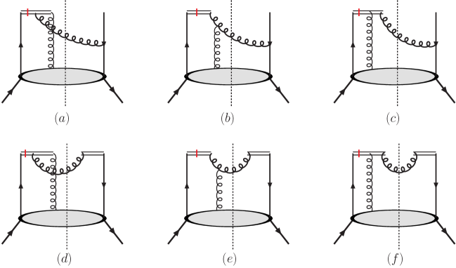
Figure 10: Same as Fig. 9, but for the hard-pole contributions.

V.2 Unpolarized Cross Section

The spin-independent cross section for the Drell-Yan process has the following TMD factorization in the regime $q_{\perp}\ll Q$ ColSopSte85 ; JiMaYu04 :

$$\frac{d^{4}\sigma}{dQ^{2}dyd^{2}q_{\perp}} = \sigma_{0}\sum_{q}e_{q}^{2}\int d^{2}\vec{k}_{1\perp}d^{2}\vec{k}_{2\perp}d^{2}\vec{\lambda}_{\perp}\delta^{(2)}(\vec{k}_{1\perp}+\vec{k}_{2\perp}+\vec{\lambda}_{\perp}-\vec{q}_{\perp})$$ (40)

$$\times\,q(z_{1},k_{1\perp},\zeta_{1})\bar{q}(z_{2},k_{2\perp},\zeta_{2})~{}H(Q^{2})\left(S(\lambda_{\perp},\rho)\right)^{-1}\ ,$$

where as before $q(z,k_{\perp})$ and $\bar{q}(z,k_{\perp})$ are the TMD quark and antiquark distributions. $H$ is a hard factor and is entirely perturbative. It is a function of $Q\gg q_{\perp}$ only. The soft-factor $S$ is a vacuum matrix element of Wilson lines and captures the effects of soft gluon radiation. Since the soft-gluon contributions in the TMD distributions have not been subtracted, the soft factor enters with inverse power. As mentioned earlier, in order to regulate the light-cone singularities, we introduce the off-light-cone vectors $v_{1}$ and $v_{2}$ for the TMD distributions. We also define $\zeta_{1}^{2}=(2v_{1}\cdot P)^{2}/v_{1}^{2}$ and $\zeta_{2}^{2}=(2v_{2}\cdot P^{\prime})^{2}/v_{2}^{2}$, and the soft-gluon rapidity cut-off $\rho=\sqrt{(2v_{1}\cdot v_{2})^{2}/v_{1}^{2}v_{2}^{2}}$. In a special coordinate frame, $z_{1}^{2}\zeta_{1}^{2}=z_{2}^{2}\zeta_{2}^{2}=\rho Q^{2}$ JiMaYu04 . There are also explicit renormalization scale dependences of the various factors in the factorization formula, which have been omitted for simplicity.

In Eq. (36) in the previous subsection, we have already given the unpolarized TMD quark distribution, calculated perturbatively for $k_{\perp}\gg\Lambda_{\rm QCD}$. Also the soft factor may be calculated in this fashion. To leading order in $\alpha_{s}$, one finds JiMaYu04 ,

$$S(\lambda_{\perp})=\delta^{(2)}(\vec{\lambda}_{\perp})+\frac{\alpha_{s}}{2\pi^{2}}\frac{1}{\vec{\lambda}_{\perp}^{2}}C_{F}\left(\ln\rho^{2}-2\right)\ .$$ (41)

By adding virtual contributions, the soft function is normalized in such a way that it obeys $\int d^{2}\vec{\lambda}_{\perp}S(\lambda_{\perp})=1$.

Inserting the perturbative TMD distribution (36) and the soft function (41) into the factorization formula (40), we find that indeed the unpolarized cross section given by Eqs. (27), (26) is reproduced, including the quark-gluon scattering piece. Here we use the above normalization condition for the soft function, and the normalization that the integration over the TMD distribution yields the normal Feynman parton distributions,

$$\int d^{2}\vec{k}_{\perp}q(z_{1},k_{\perp})=q(z_{1})\ ,\quad\int d^{2}\vec{k}_{\perp}\bar{q}(z_{2},k_{\perp})=\bar{q}(z_{2})\ .$$ (42)

V.3 Polarized Cross Section

In JiMaYu04 also a factorization formula for the transverse-spin dependent Drell-Yan cross section at $q_{\perp}\ll Q$ was established, which reads:

$$\frac{d^{4}\Delta\sigma(S)}{dQ^{2}dyd^{2}q_{\perp}} = \sigma_{0}\,\epsilon^{\alpha\beta}{S}_{\perp\alpha}\,q_{\perp\beta}\frac{1}{M_{P}}\int d^{2}\vec{k}_{1\perp}d^{2}\vec{k}_{2\perp}d^{2}\vec{\lambda}_{\perp}~{}\frac{\vec{k}_{1\perp}\cdot\vec{q}_{\perp}}{q_{\perp}^{2}}~{}\delta^{(2)}(\vec{k}_{1\perp}+\vec{k}_{2\perp}+\vec{\lambda}_{\perp}-\vec{q}_{\perp})$$ (43)

$$\times q_{T}(z_{1},k_{1\perp},\zeta_{1})~{}\bar{q}(z_{2},k_{2\perp},\zeta_{2})~{}H(Q^{2})\left(S(\lambda_{\perp})\right)^{-1}\ ,$$

where $q_{T}(z,k_{\perp})$ is the Sivers function defined in Eq. (35), $\bar{q}(z,k_{\perp})$ is again the anti-quark TMD for the unpolarized proton, and $H$ and $S$ are the hard and soft factors introduced earlier.

We have given the first-order perturbative result for the Sivers function in Eq. (39). As was shown in BoeMulPij03 (see also MaWa03 ; bacchetta ), its $k_{\perp}^{2}$-moment is related to the twist-three quark-gluon correlation function defined in Eq. (3) of Sec. II:

$$\frac{1}{M_{P}}\int d^{2}\vec{k}_{\perp}\vec{k}_{\perp}^{2}q_{T}(x,k_{\perp})=T_{F}(x,x)\ .$$ (44)

For deep-inelastic scattering, this relation remains true, except that the sign will be opposite. Inserting finally all TMD functions into the factorization formula (43), we reproduce the differential Drell-Yan single-transverse-spin cross section given at low transverse momentum in Eqs. (31), (28) of Sec. IV. This concludes our demonstration that the ETQS mechanism and the approach based on TMD factorization produce identical results in the kinematic regime where they overlap.

VI Summary and Outlook

In summary, we have studied the single-transverse-spin asymmetry in Drell-Yan pair production at large and moderate transverse momenta. At large transverse momenta $q_{\perp}\sim Q$, the asymmetry is power-suppressed by $1/Q$. Therefore, the collinear-factorized approach based on twist-three quark-gluon correlations should provide the appropriate description. We have used this approach to derive the single-spin asymmetry. We have then expanded the result for moderate transverse momenta of the lepton pair, $\Lambda_{\rm QCD}\ll q_{\perp}\ll Q$. In this regime, one knows that a factorization theorem in terms of transverse-momentum dependent parton distributions holds, involving in particular the Sivers function. We have verified that indeed a smooth transition from the higher-twist mechanism to the one based on TMD factorization occurs, with the two approaches describing the same physics in the region of overlap. This unifies the two approaches, and provides input for new strategies in the analysis of experimental data for single-spin asymmetries.

In qiu , it was noted that there are additional twist-three quark-gluon correlation functions that may contribute to the SSAs in hard processes. One of them is a spin-averaged and chiral-odd correlation, defined by qiu

$$T_{F}^{(\sigma)}(x_{1},x_{2})=\int\frac{d\zeta^{-}d\eta^{-}}{8\pi}e^{ix_{1}P^{+}\eta^{-}}e^{i(x_{2}-x_{1})P^{+}\zeta^{-}}\left\langle P|\overline{\psi}(0)\sigma^{+\alpha}gF^{+\alpha}(\zeta^{-})\psi(\eta^{-})|P\right\rangle\ .$$ (45)

When combined with the quark transversity distribution for the polarized proton, the above correlation in the unpolarized proton can also contribute to the SSA for the Drell-Yan process at large transverse momentum. However, after a straightforward calculation we find that the contribution vanishes in the low transverse momentum limit $q_{\perp}\ll Q$. This observation is consistent with the TMD factorization at low transverse momentum JiMaYu04 , where only the Sivers function contributes to the SSA for the Drell-Yan process after integration over the lepton angles.

There are a number of directions in which our work could be extended. First, an interesting topic will be to study the single-spin asymmetry in semi-inclusive deep inelastic scattering (SIDIS) $ep\to e\pi X$ yuji , again at large and moderate transverse momenta of the final-state hadron. Also here, a connection between the twist-three mechanism and the TMD factorization formalism can be established. The Sivers function calculated perturbatively in this paper may be immediately applied to SIDIS, after changing its sign. Although the calculation for SIDIS should be straightforward following our derivations for the Drell-Yan process in this paper, the details will differ. It will be crucial to demonstrate that the two approaches are indeed also consistent for the SIDIS process at $\Lambda_{\rm QCD}\ll q_{\perp}\ll Q$, and to explicitly verify the process-dependence for the single-transverse spin asymmetries in hard processes. It also needs to be demonstrated that the Collins function mechanism collins can be reproduced in the low-$q_{\perp}$ region. We will present a study of SIDIS in a future publication.

Second, the consistency between the twist-three and the TMD factorization approaches should also lead the way to resumming the large logarithms from higher-order soft gluon radiation. As shown in Eq.(28)-(30), the first-order expressions contain a large logarithm $\propto\ln Q^{2}/q_{\perp}^{2}$. This large logarithm will be present in higher orders, with two additional powers of the logarithm at every new order in perturbation. In order to have a reliable theoretical calculation, these logarithms need to be resummed. The resummation procedure may follow the classic example in ColSopSte85 for the unpolarized Drell-Yan cross section. The relevant Collins-Soper equation for the energy evolution of the spin-dependent TMD quark distributions has already been derived in IdiJiMaYu04 . The resummation effects will be particularly important at small $q_{\perp}/Q$.

References

- (1) see for example: G. Bunce et al., Phys. Rev. Lett. 36, 1113 (1976); D. L. Adams et al. [E581 and E704 Collaborations], Phys. Lett. B 261, 201 (1991); D. L. Adams et al. [FNAL-E704 Collaboration], Phys. Lett. B 264, 462 (1991); K. Krueger et al., Phys. Lett. B 459, 412 (1999).
- (2) A. Bravar [Spin Muon Collaboration], Nucl. Phys. A 666, 314 (2000); A. Airapetian et al. [HERMES Collaboration], Phys. Rev. Lett. 84, 4047 (2000); A. Airapetian et al. [HERMES Collaboration], Phys. Rev. D 64, 097101 (2001); Phys. Rev. Lett. 94, 012002 (2005); M. Diefenthaler [HERMES Collaboration], arXiv:hep-ex/0507013; H. Avakian [CLAS Collaboration], talk presented at the RBRC workshop “Single-Spin Asymmetries”, Brookhaven National Laboratory, Upton, New York, June 1-3, 2005, to appear in the proceedings; V. Y. Alexakhin et al. [COMPASS Collaboration], Phys. Rev. Lett. 94, 202002 (2005).
- (3) J. Adams et al. [STAR Collaboration], Phys. Rev. Lett. 92, 171801 (2004); S. S. Adler [PHENIX Collaboration], Phys. Rev. Lett. 95, 202001 (2005); F. Videbaek [BRAHMS Collaboration], AIP Conf. Proc. 792, 993 (2005); arXiv:nucl-ex/0601008.
- (4) for reviews, see: M. Anselmino, A. Efremov and E. Leader, Phys. Rept. 261, 1 (1995) [Erratum-ibid. 281, 399 (1997)]; Z. t. Liang and C. Boros, Int. J. Mod. Phys. A 15, 927 (2000); V. Barone, A. Drago and P. G. Ratcliffe, Phys. Rept. 359, 1 (2002);
- (5) D. W. Sivers, Phys. Rev. D 41, 83 (1990); Phys. Rev. D 43, 261 (1991).
- (6) A. V. Efremov and O. V. Teryaev, Sov. J. Nucl. Phys. 36, 140 (1982) [Yad. Fiz. 36, 242 (1982)]; A. V. Efremov and O. V. Teryaev, Phys. Lett. B 150, 383 (1985).
- (7) J.W. Qiu and G. Sterman, Phys. Rev. Lett. 67, 2264 (1991); Nucl. Phys. B 378, 52 (1992); Phys. Rev. D 59, 014004 (1999).
- (8) Y. Kanazawa and Y. Koike, Phys. Lett. B 478, 121 (2000); Phys. Rev. D 64, 034019 (2001).
- (9) M. Anselmino, M. Boglione and F. Murgia, Phys. Lett. B 362, 164 (1995); M. Anselmino and F. Murgia, Phys. Lett. B 442, 470 (1998); U. D’Alesio and F. Murgia, Phys. Rev. D 70, 074009 (2004); M. Anselmino, M. Boglione, U. D’Alesio, E. Leader, S. Melis and F. Murgia, Phys. Rev. D 73, 014020 (2006).
- (10) P. J. Mulders and R. D. Tangerman, Nucl. Phys. B 461, 197 (1996) [Erratum-ibid. B 484, 538 (1997)]; D. Boer and P. J. Mulders, Phys. Rev. D 57, 5780 (1998).
- (11) see for example, M. Anselmino et al., arXiv:hep-ph/0511017, and references therein.
- (12) J. C. Collins and D. E. Soper, Nucl. Phys. B 193, 381 (1981) [Erratum-ibid. B 213, 545 (1983)]; Nucl. Phys. B 197, 446 (1982); J. C. Collins and D. E. Soper, Nucl. Phys. B 194, 445 (1982).
- (13) J. C. Collins, D. E. Soper and G. Sterman, Nucl. Phys. B 250, 199 (1985).
- (14) X. Ji, J. P. Ma and F. Yuan, Phys. Rev. D 71, 034005 (2005); X. Ji, J. P. Ma and F. Yuan, Phys. Lett. B 597, 299 (2004).
- (15) J. C. Collins and A. Metz, Phys. Rev. Lett. 93, 252001 (2004).
- (16) S. J. Brodsky, D. S. Hwang and I. Schmidt, Phys. Lett. B 530, 99 (2002); Nucl. Phys. B 642, 344 (2002).
- (17) J. C. Collins, Phys. Lett. B 536, 43 (2002).
- (18) X. Ji and F. Yuan, Phys. Lett. B 543, 66 (2002); A. V. Belitsky, X. Ji and F. Yuan, Nucl. Phys. B 656, 165 (2003).
- (19) D. Boer, P. J. Mulders and F. Pijlman, Nucl. Phys. B 667, 201 (2003).
- (20) C. J. Bomhof, P. J. Mulders and F. Pijlman, Phys. Lett. B 596, 277 (2004); A. Bacchetta, C. J. Bomhof, P. J. Mulders and F. Pijlman, Phys. Rev. D 72, 034030 (2005); C. J. Bomhof, P. J. Mulders and F. Pijlman, arXiv:hep-ph/0601171.
- (21) X. Ji, J. W. Qiu, W. Vogelsang and F. Yuan, arXiv:hep-ph/0602239.
- (22) J. P. Ma and Q. Wang, Eur. Phys. J. C 37, 293 (2004).
- (23) A. Bacchetta, arXiv:hep-ph/0511085.
- (24) X. D. Ji, Phys. Lett. B 289, 137 (1992).
- (25) M. Luo, J. W. Qiu and G. Sterman, Phys. Rev. D 50, 1951 (1994).
- (26) X. Guo, Phys. Rev. D 58, 036001 (1998); Nucl. Phys. A 638, 539C (1998).
- (27) see also: P. G. Ratcliffe, Eur. Phys. J. C 8, 403 (1999).
- (28) R. Meng, F. I. Olness and D. E. Soper, Phys. Rev. D 54, 1919 (1996).
- (29) E. Laenen, G. Sterman and W. Vogelsang, Phys. Rev. D 63, 114018 (2001).
- (30) X. Ji, J. P. Ma and F. Yuan, JHEP 0507, 020 (2005).
- (31) G. Altarelli, R. K. Ellis, M. Greco and G. Martinelli, Nucl. Phys. B 246, 12 (1984).
- (32) Y. Koike, talk given at the RIKEN/BNL Research Center Workshop on “Single-Spin Asymmetries”, Brookhaven National Laboratory, Upton, New York, June 1-3, 2005; H. Eguchi, Y. Koike, K. Tanaka, arXiv:hep-ph/0604003.
- (33) J. C. Collins, Nucl. Phys. B 396, 161 (1993).
- (34) A. Idilbi, X. Ji, J. P. Ma and F. Yuan, Phys. Rev. D 70, 074021 (2004).