High Density Quark Matter and the Renormalization Group
in QCD with two and three Flavors

Abstract

We consider the most general four fermion operators in QCD for two and three massless flavors and study their renormalization in the vicinity of the Fermi surface. We show that, asymptotically, the largest coupling corresponds to scalar diquark condensation. Asymptotically the direct and iterated (molecular) instanton interactions become equal. We provide simple arguments for the form of the operators that diagonalize the evolution equations. Some solutions of the flow equations exhibit instabilities arising out of purely repulsive interactions.

1. Recently there has been renewed interest in the problem of hadronic matter at high baryon density. It was realized early on that at very high density, asymptotic freedom and the presence of a Fermi surface implies that attractive interactions between quarks cause a BCS instability, and cold quark matter is a color superconductor [1]. More recently, the problem was studied again, and it was emphasized that non-perturbative effects, instantons, could lead to gaps on the order of 100 MeV [2, 3]. A particularly interesting case is QCD with three light flavors. In this case the preferred order parameter involves a coupling between color and flavor degrees of freedom [4]. The resulting coherence leads to large gaps even for weak interactions. In addition to that, color-flavor locking implies that chiral symmetry is broken. The usual quark condensate is non-vanishing even in the high density phase, as is a gauge-invariant $\Delta B=2$ condensate, signalling true superfluidity [4, 5].

Most of these calculations were performed in the mean field approximation. (In the instanton model, a number of refinements have been included, see [6, 5].) One assumes a specific form of the interaction (instantons, one gluon exchange, $\ldots$), makes an ansatz for the form of the condensate, and solves the gap equation in some approximation. Clearly, it is desirable to analyze the structure of the theory for the most general form of the interaction, and to have a guiding principle for constructing a systematic expansion scheme.

In this context, the renormalization group approach to cold Fermi systems appears particularly promising [7, 8]. In a cold Fermi system, the only relevant interactions take place in vicinity of the Fermi surface. The corresponding excitations are quasi-particles and quasi-holes, described by an effective action of the form

$$S_{eff} = \int dt\,d^{3}p\;\psi^{\dagger}\left(i\partial_{t}-(\epsilon(p)-\epsilon_{F})\right)\psi.$$ (1)

We can analyze the general structure of the quasi-particle interactions by studying the evolution of the corresponding operators as we successfully integrate out modes closer and closer to the Fermi surface. The main result of this analysis is that, in general, four fermion, six fermion, and higher order interactions are suppressed as we approach the Fermi surface. This fixed point corresponds to Landau liquid theory [9]. The only exception is the four-fermion operator that corresponds to two particles from opposite corners of the Fermi surface $(p_{F},-p_{F})$ scattering into $(p^{\prime}_{F},-p^{\prime}_{F})$. This kind of scattering leads to a logarithmic growth of the coupling constant as we approach the Fermi surface, and the well known BCS instability.

2. For QCD, this approach was first employed by Evans, Hsu, and Schwetz [10]. These authors concentrated on the one gluon exchange interaction, but as we will see in a moment, their results are sufficient to deal with the most general quark-quark interaction for QCD with three (or more) flavors. We should emphasize here that we will restrict ourselves to massless QCD, a spherical Fermi surface, and local operators invariant under the appropriate chiral symmetry.

Following [10], we take the basic four fermion operators in $N_{f}=3$ QCD to be

$$O^{0}_{LL} = (\bar{\psi}_{L}\gamma_{0}\psi_{L})^{2},\hskip 28.45274ptO^{0}_{LR}\;=\;(\bar{\psi}_{L}\gamma_{0}\psi_{L})(\bar{\psi}_{R}\gamma_{0}\psi_{R})$$ (2)

$$O^{i}_{LL} = (\bar{\psi}_{L}\gamma_{i}\psi_{L})^{2},\hskip 28.45274ptO^{i}_{LR}\;=\;(\bar{\psi}_{L}\vec{\gamma}\psi_{L})(\bar{\psi}_{R}\vec{\gamma}\psi_{R}).$$ (3)

Each of these operators comes in two color structures, for example color symmetric and color anti-symmetric

$$(\bar{\psi}^{a}\psi^{b})(\bar{\psi}^{c}\psi^{d})\left(\delta_{ab}\delta_{cd}\pm\delta_{ad}\delta_{bc}\right).$$ (4)

Nothing essentially new emerges from considering superficially different isospin structures, or different Dirac matrices. All such structures can be reduced to linear combinations of the basic ones (2), or their parity conjugates, by Fierz rearrangements. In total, we have to consider eight operators.

These operators are renormalized by quark-quark scattering in the vicinity of the Fermi surface. This means that both incoming and outgoing quarks have momenta $\vec{p}_{1},\vec{p}_{2}\simeq\pm\vec{p}$ and $\vec{p}_{3},\vec{p}_{4}\simeq\pm\vec{q}$ with $|\vec{p}|,|\vec{q}|\simeq p_{F}$. We can take the external frequency to be zero. A graph with vertices $\Gamma_{1}$ and $\Gamma_{2}$ then gives [10]

$$G_{1}G_{2}I\;(\Gamma_{1})_{i^{\prime}i}(\Gamma_{1})_{k^{\prime}k}\left[-(\gamma_{0})_{ij}(\gamma_{0})_{kl}-\frac{1}{3}(\vec{\gamma})_{ij}(\vec{\gamma})_{kl}\right](\Gamma_{2})_{jj^{\prime}}(\Gamma_{2})_{ll^{\prime}}$$ (5)

with $I=\frac{i}{8\pi^{2}}\mu^{2}\log(\Lambda_{IR}/\Lambda_{UV})$. Here $[\Lambda_{IR},\Lambda_{UV}]$ is the range of momenta that was integrated out. We will denote the density of states on the Fermi surface by $N=\mu^{2}/(2\pi^{2})$ and the logarithm of the scale $t=\log(\Lambda_{IR}/\Lambda_{UV})$ as in [10]. The renormalization group does not mix $LL$ and $LR$ operators, and it also does not mix different color structures. This means that the evolution equations contain at most $2\times 2$ blocks. For completeness, we reproduce the results of [10]

$$\frac{d(G^{LL}_{0}+G^{LL}_{i})}{dt} = -\frac{N}{3}(G^{LL}_{0}+G^{LL}_{i})^{2}$$ (6)

$$\frac{d(G^{LL}_{0}-3G^{LL}_{i})}{dt} = -N(G^{LL}_{0}-3G^{LL}_{i})^{2}$$ (7)

$$\frac{d(G^{LR}_{0}+3G^{LR}_{i})}{dt} = 0$$ (8)

$$\frac{d(G^{LR}_{0}-G^{LR}_{i})}{dt} = -\frac{2N}{3}(G^{LR}_{0}-G^{LR}_{i})^{2}$$ (9)

In this basis the evolution equations are already diagonal. The coupling $G_{1}=G^{LL}_{0}+G^{LL}_{i}$ evolves as

$$G_{1}(t) = \frac{1}{1+(N/3)G_{1}(0)t}$$ (10)

with analogous results for the other operators. Note that the evolution starts at $t=0$ and moves towards the Fermi surface $t\to-\infty$. If the coupling is attractive at the matching scale, $G_{1}(0)>0$, it will grow during the evolution, and reach a Landau pole at $t_{c}=3/(NG_{1}(0))$. The location of the pole is controlled by the initial value of the coupling and the coefficient in the evolution equation. If the initial coupling is negative, the coupling decreases during the evolution. The second operator in (6) has the largest coefficient and will reach the Landau pole first, unless the initial value is very small or negative. In this case, subdominant operators may dominate the pairing.

The particular form of the operators that diagonalize the evolution equations is easily understood. Let us first order the operators according to the size of the coefficient in the evolution equations

$$O_{dom} = (\bar{\psi}_{L}\gamma_{0}\psi_{L})^{2}-(\bar{\psi}_{L}\vec{\gamma}\psi_{L})^{2},$$ (11)

$$O_{sub,1} = (\bar{\psi}_{L}\gamma_{0}\psi_{L})(\bar{\psi}_{R}\gamma_{0}\psi_{R})-\frac{1}{3}(\bar{\psi}_{L}\vec{\gamma}\psi_{L})(\bar{\psi}_{R}\vec{\gamma}\psi_{R}),$$ (12)

$$O_{sub,2} = (\bar{\psi}_{L}\gamma_{0}\psi_{L})^{2}+\frac{1}{3}(\bar{\psi}_{L}\vec{\gamma}\psi_{L})^{2},$$ (13)

$$O_{mar} = (\bar{\psi}_{L}\gamma_{0}\psi_{L})(\bar{\psi}_{R}\gamma_{0}\psi_{R})+(\bar{\psi}_{L}\vec{\gamma}\psi_{L})(\bar{\psi}_{R}\vec{\gamma}\psi_{R}).$$ (14)

This result can be made more transparent by Fierz rearranging the operators. We find

$$O_{dom} = 2(\psi_{L}C\psi_{L})(\bar{\psi}_{L}C\bar{\psi}_{L}),$$ (15)

$$O_{sub,1} = \frac{1}{3}(\psi_{L}C\vec{\gamma}\psi_{R})(\bar{\psi}_{R}C\vec{\gamma}\psi_{L})+\ldots,$$ (16)

$$O_{sub,2} = \frac{4}{3}(\psi_{L}C\vec{\Sigma}\psi_{L})(\bar{\psi}_{L}C\vec{\Sigma}\bar{\psi}_{L}),$$ (17)

$$O_{mar} = \frac{1}{2}(\psi_{L}C\gamma_{0}\psi_{R})(\bar{\psi}_{R}C\gamma_{0}\psi_{L})+\ldots.$$ (18)

This demonstrates that the linear combinations in (11-14) correspond to simple structures in the quark-quark channel. It also means that it might have been more natural to perform the whole calculation directly in a basis of diquark operators.

The full structure of the $(LR)$ operators is $O_{sub,1},O_{mar}=(\psi C\gamma\tau_{S,A}\psi)(\bar{\psi}C\gamma\tau_{S,A}\bar{\psi})+(\psi C\gamma\gamma_{5}\tau_{A,S}\psi)(\bar{\psi}C\gamma\gamma_{5}\tau_{A,S}\bar{\psi})$ where $\tau_{S,A}$ are symmetric/anti-symmetric isospin generators. Note that because the two structures have different flavor symmetry, the flavor structure cannot be factored out.

The dominant operator corresponds to pairing in the scalar diquark channel, while the subdominant operators contain vector diquarks. Note that from the evolution equation alone we cannot decide what the preferred color channel is. To decide this question, we must invoke the fact that “reasonable” interactions, like one gluon exchange, are attractive in the color anti-symmetric repulsive in the color symmetric channel. Indeed, it is the color anti-symmetric configuration that minimizes the total color flux emanating from the quark pair. If the color wave function is anti-symmetric, the dominant operator fixes the isospin wave function to be anti-symmetric as well.

The dominant operator does not distinguish between scalar and pseudoscalar diquarks. Indeed, for $N_{f}\geq 3$ the basic 4-quark operators consistent with chiral symmetry also exhibit an accidental axial baryon symmetry, under which scalar and pseduscalar diquarks are equivalent. For $N_{f}=3$ this degeneracy is lifted by (formally irrelevant) six-fermion operators [5]. The form of the dominant operator indicates the existence of potential instabilities, but does not itself indicate how they are resolved. For example, to see whether color-flavor locking [4] is important we should use the operator as input to a variational calculation.

3. For two flavors, we have to take into account additional operators. At first hearing it might seem odd that with fewer basic entities we encounter more basic operators. It occurs because for $N_{f}=2$, but not for larger values, two quarks of the same chirality can form a chiral $SU(2)\times SU(2)$ singlet. Related to this, for $N_{f}=2$ we have additional $U(1)_{A}$ violating four fermion operators. These operators are induced by instantons.

For $N_{f}=3$, instantons are six fermion operators, and they are irrelevant in the technical sense. This does not mean they are physically irrelevant, particularly since they break a residual symmetry. The formation of the gap will cause the evolution of the couplings to stop, and the instanton coupling remains at a finite value. Instantons have important physical effects, even for $N_{f}=3$ [5]. Most notably, instantons cause quark-antiquark pairs to condense (even in the high density phase), and lift the degeneracy between the scalar and pseudoscalar diquark condensates.

The new operators are

$$O_{S} = \det_{f}(\bar{\psi}_{R}\psi_{L}),\hskip 28.45274ptO_{T}\;=\;\det_{f}(\bar{\psi}_{R}\vec{\Sigma}\psi_{L})$$ (19)

Both operators are determinants in flavor space. For quark-quark scattering, this implies that the two quarks have to have different flavors. The fact that the flavor structure is fixed implies that the color structure is fixed, too. For a given $(qq)$ spin, only one of the two color structures contributes. Finally, both quarks have to have the same chirality, and the chirality is flipped by the interaction.

These considerations determine the structure of the evolution equations (see Fig. 1). Two left handed quarks can interact via one of the instanton operators, become right handed, and then rescatter through an anti-instanton, or through one of the $U(1)_{A}$ symmetric $RR$ operators. The result will be a renormalization of the $LL$ vertex in the first case, and a renormalization of the instanton in the second. The iterated instanton-anti-instanton interaction was discussed in great detail in [11], and was argued to play an important role in the high temperature [11] and high density phase of QCD [5]. We should note that the flavor structure will always remain a determinant. Even though instantons generate all the Dirac structures in (2), the color-flavor structure is more restricted.

Evidently, instantons do not affect the evolution of the $LR$ couplings at all. The evolution equations of the $LL$ couplings are modified to become (henceforth we drop the subscript $LL$ from):

$$\frac{dG_{0}}{dt} = \frac{N}{2}\Bigg{\{}-G_{0}^{2}+2G_{0}G_{i}-5G_{i}^{2}-K_{S}^{2}+2K_{S}K_{T}-5K_{T}^{2}\Bigg{\}}$$ (20)

$$\frac{dG_{i}}{dt} = \frac{N}{2}\Bigg{\{}\frac{1}{3}G_{0}^{2}-\frac{10}{3}G_{0}G_{i}+\frac{13}{3}G_{i}^{2}+\frac{1}{3}K_{S}^{2}-\frac{10}{3}K_{S}K_{T}+\frac{13}{3}K_{T}^{2}\Bigg{\}}$$ (21)

$$\frac{dK_{S}}{dt} = \frac{N}{2}\Bigg{\{}2\left(-G_{0}+G_{i}\right)K_{S}+2\left(G_{0}-5G_{i}\right)K_{T}\Bigg{\}}$$ (22)

$$\frac{dK_{T}}{dt} = \frac{N}{2}\Bigg{\{}\frac{2}{3}\left(G_{0}-5G_{i}\right)K_{S}+\frac{2}{3}\left(-5G_{0}+13G_{i}\right)K_{T}\Bigg{\}}$$ (23)

These equations can be decoupled as

$$\frac{dG_{1}}{dt} = -\frac{N}{3}\left(G_{1}^{2}+K_{1}^{2}\right),$$ (24)

$$\frac{dK_{1}}{dt} = -\frac{2N}{3}\;G_{1}K_{1},$$ (25)

$$\frac{dG_{2}}{dt} = -N\left(G_{2}^{2}+K_{2}^{2}\right),$$ (26)

$$\frac{dK_{2}}{dt} = -2N\;G_{2}K_{2},$$ (27)

where $G_{1}=G_{0}+G_{i},K_{1}=K_{S}+K_{T}$ and $G_{2}=G_{0}-3G_{i},K_{2}=K_{S}-3K_{T}$. The equations for $G,K$ decouple even further. We have

$$\frac{d(G_{2}+K_{2})}{dt} = -N\left(G_{2}+K_{2}\right)^{2}$$ (28)

$$\frac{d(G_{2}-K_{2})}{dt} = -N\left(G_{2}-K_{2}\right)^{2},$$ (29)

as well as the analogous equation for $G_{1},K_{1}$. These differential equations are now trivial to solve, leading to

$$G_{2}(t) = \frac{1}{2}\left\{\frac{1}{a+Nt}+\frac{1}{b+Nt}\right\},$$ (30)

$$K_{2}(t) = \frac{1}{2}\left\{\frac{1}{a+Nt}-\frac{1}{b+Nt}\right\},$$ (31)

again with the analogous result holding for $G_{1},K_{1}$. Here, $a,b=(G_{2}(0)\pm K_{2}(0))^{-1}$. The result implies that $G_{2}$ and $K_{2}$ will grow and eventually reach a Landau pole if either $a$ or $b$ is positive. The location of the pole is determined by the smaller of the values, $t_{c}=-a/N$ or $t_{c}=-b/N$. The same is true for $G_{1}$ and $K_{1}$, but the couplings evolve more slowly, and the Landau pole is reached later.

At this level a number of qualitatively different scenarios are possible, depending on the sign and relative magnitude of $G(0)$ and $K(0)$, see Fig. 2 (henceforth we drop all subscripts). If $G(0)$ and $K(0)$ are both positive then they will both grow, and the location of the nearest Landau pole is determined by $G(0)+K(0)$. The asymptotic ratio of the two couplings is 1. If $G(0)$ and $K(0)$ are both negative, and the magnitude of $G(0)$ is bigger than the magnitude of $K(0)$, then the evolution drives both couplings to zero. These are the standard cases. Attraction leads to an instability, and repulsive forces are suppressed.

More interesting cases arise when the sign of the two couplings is different. The case $G(0),K(0)<0$ and $|K(0)|>|G(0)|$ is especially weird. Both $G(0),K(0)$ are repulsive, but the evolution drives $G(0)$ to positive values. Both couplings reach a Landau pole, and near the pole their asymptotic ratio approaches minus one. Similarly, we can have a negative $G(0)$ and positive $K(0)$ with $K(0)>|G(0)|$. Again, the evolution will drive $G(0)$ to positive values.

4. The dominant and sub-dominant instanton operators are

$$O_{dom} = \det_{f}\left[(\bar{\psi}_{R}\psi_{L})^{2}-(\bar{\psi}_{R}\vec{\Sigma}\psi_{L})^{2}\right],$$ (32)

$$O_{sub} = \det_{f}\left[(\bar{\psi}_{R}\psi_{L})^{2}+\frac{1}{3}(\bar{\psi}_{R}\vec{\Sigma}\psi_{L})^{2}\right].$$ (33)

Upon Fierz rearrangement, we find

$$O_{dom} = 2(\psi_{L}C\tau_{2}\psi_{L})(\bar{\psi}_{R}C\tau_{2}\bar{\psi}_{R}),$$ (34)

$$O_{sub} = \frac{2}{3}(\psi_{L}C\tau_{2}\vec{\Sigma}\psi_{L})(\bar{\psi}_{R}C\tau_{2}\vec{\Sigma}\bar{\psi}_{R}),$$ (35)

corresponding to scalar and tensor diquarks. Both operators are flavor singlet. Overall symmetry then fixes the color wave functions, anti-symmetric $\bar{3}$ for the scalar, and symmetric 6 for the tensor. The dominant pairing induced by instantons is in the scalar diquark channel, the only other attractive channel is the tensor. All this neatly confirms the scenario discussed in [2, 3]. Note that condensation in the tensor channel violates rotational symmetry. As a result, the gap equation has additional suppression factors and the gap is very small [2].

Just as we found for $N_{f}\geq 3$, there is an appealing heuristic understanding for the amazingly simple behavior of the evolution equations, obtained by focussing on the diquark channels. Instantons distinguish between scalar diquarks with positive and negative parity. $G+K$ corresponds to the positive parity operator $(\psi C\gamma_{5}\psi)$ and $G-K$ to the negative parity $(\psi C\psi)$. The asymptotic approach of $G/K\to 1$, then corresponds to the fact that scalar diquark condensation is favored over pseudoscalar diquark condensation. This is always the case if $K(0)>0$. We also understand the strange case $G(0),K(0)<0$ and $|K(0)|>|G(0)|$. In this case the interaction for scalar diquarks is repulsive, but the interaction in the pseudoscalar channel is attractive and leads to an instability. Note that this can only happen if we have the “wrong” sign of the instanton interaction, i.e. for $\theta=\pi$. Similarly, we can understand why the asymptotic ratio of the molecular (instanton-anti-instanton) and direct instanton couplings approaches $G/K=\pm 1$. Instantons induce a repulsive interaction for pseudoscalar diquarks. During the evolution, this coupling will be suppressed, whereas the attractive scalar interaction grows. But this means that in the pseudoscalar channel, the repulsive (instanton) and attractive (molecular) forces have to cancel in the asymptotic limit, so the effective couplings become equal.

We have not made an attempt to match all the coupling constants to a realistic model at the UV scale. To do so would require an understanding of the instanton density, the relevant value of $\alpha_{s}$, the screening mechanism, and many other things. From the form of the instanton vertex we can fix the ratio of the two instanton-like couplings, $K_{T}/K_{S}=1/(2N_{c}-1)$ [12, 13]. This again shows that the tensor channel is not expected to be important. Also, both one gluon exchange and higher order instanton effects give $G^{LL}_{0}>0,-G^{LL}_{i}>0$. Thus the favored scenario is that both instanton and $U(1)_{A}$ symmetric couplings flow at the same rate, and pairing is dominated by scalar diquarks.

5. In summary, we find that the renormalization group analysis broadly supports the findings of [2, 3]. The dominant coupling corresponds to scalar diquark condensation, the sub-dominant coupling to tensor diquarks. Asymptotically, $U(1)_{A}$ breaking and $U(1)_{A}$ symmetric couplings flow at the same rate. Since instantons have a definite isospin structure, there is one flavor symmetric coupling that evolves independently of instantons. Asymptotically, this coupling also flows at the same rate. In principle there is the possibility of flavor and color symmetric diquark condensates, but none of the model interactions so far proposed is attractive in that channel.

The analysis presented here is incomplete in several ways. Realistic interactions (one-gluon exchange, instantons, $\ldots$) are momentum dependent, and that should be included in the evolution. This complication is particularly important for one-gluon exchange, because in perturbation theory the diagram is not completely screened, and has a divergence for small momentum transfers. For $N_{f}=3$ a self-consistent calculation ought to be possible, because color-flavor locking completely screens the interaction.

In any case, the renormalization group only determines the running of the couplings from the matching point down to some infrared scale. If a subdominant coupling is unusually large at the matching scale, it might still dominate the pairing. To decide the form of the pairing and determine the gap, given the couplings, still requires a variational calculation along the lines of [4, 5].

Acknowledgments: After this work was begun, we learned that the authors of [10] have also extended their study to include instanton operators. This work was supported in part by NSF-PHY-9513835.

FIG. 1.: Chiral structure of the evolution equations.

FIG. 2.: Solutions to the evolution equations for cases with different relative strength of the $U(1)_{A}$ violating interaction $K$ (dashed line) and $U(1)_{A}$ conserving interaction $G$ (solid line).

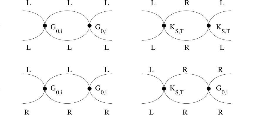
FIG. 1.:

FIG. 2.:

REFERENCES

- [1] D. Bailin and A. Love, Phys. Rep. 107, 325 (1984) .
- [2] M. Alford, K. Rajagopal, and F. Wilczek, Phys. Lett. B422 247 (1998).
- [3] R. Rapp, T. Schäfer, E. V. Shuryak, and M. Velkovsky, Phys. Rev. Lett. 81 (1998) 53.
- [4] M. Alford, K. Rajagopal, and F. Wilczek, hep-ph/9804403.
- [5] R. Rapp, T. Schäfer, E. V. Shuryak, and M. Velkovsky, in preparation.
- [6] G.W. Carter and D. Diakonov, hep-ph/9807219.
- [7] J. Polchinski, hep-th/9210046.
- [8] R. Shankar, Rev. Mod. Phys. 66, 129 (1995)
- [9] A. A. Abrikosov, L. P. Gorkov, and I. E. Dzyaloshinski, ’Methods of Quantum Field Theory in Statistical Phsysics’, Prentice Hall, Englewood Cliffs, New Jersey 1963.
- [10] N. Evans, S. Hsu, and M. Schwetz, hep-ph/9808444.
- [11] T. Schäfer, E. V. Shuryak, and J. J. M. Verbaarschot, Phys. Rev. D51 (1995) 1267.
- [12] M. A. Shifman, A. I. Vainshtein, and V. I. Zakharov, Nucl. Phys. B163, 46 (1980).
- [13] T. Schäfer and E. V. Shuryak, Rev. Mod. Phys. 70, 323 (1998).