QCD in Extreme Conditions
and the
Wilsonian ‘Exact Renormalization Group’

Abstract

This is an introduction to the use of nonperturbative flow equations in strong interaction physics at nonzero temperature and baryon density. We investigate the QCD phase diagram as a function of temperature, chemical potential for baryon number and quark mass within the linear quark meson model for two flavors. Whereas the renormalization group flow leads to spontaneous chiral symmetry breaking in vacuum, the symmetry is restored in a second order phase transition at high temperature and vanishing quark mass. We explicitly connect the physics at zero temperature and realistic quark mass with the universal behavior near the critical temperature $T_{c}$ and the chiral limit. At high density we find a chiral symmetry restoring first order transition. The results imply the presence of a tricritical point with long-range correlations in the phase diagram. We end with an outlook to densities above the chiral transition, where QCD is expected to behave as a color superconductor at low temperature.

Based on five lectures presented at the 11th Summer School and Symposium on Nuclear Physics “Effective Theories of Matter”, Seoul National University, June 23–27, 1998.

Contents

toc

I Overview

These lectures are about some recent developments concerning the physics of the strong interaction, Quantumchromodynamics (QCD), in extremes of temperature and baryon density. Here “extremes” means temperatures of the order of $10^{12}\,$K or $100\,{\rm MeV}$ and densities of about a few times nuclear matter density $n_{0}=0.153\,{\rm fm}^{-3}=(105\,{\rm MeV})^{3}$.

The following schematic phase diagram gives an idea about what the behavior of QCD in thermal and chemical equilibrium may look like as a function of temperature and chemical potential of quark number density. We will use it here to draw the attention to some aspects which will be explained in more detail in these lectures and to point out their experimental relevance.

Shortly after the discovery of asymptotic freedom [2], it was realized [3] that at sufficiently high temperature or density QCD may differ in important aspects from the corresponding zero temperature or vacuum properties. If one considers the phase structure of QCD as a function of temperature one expects around a critical temperature of $T_{c}\simeq 150\,{\rm MeV}$ two qualitative changes. First, the quarks and gluons which are confined into hadrons at zero temperature can be excited independently at sufficiently high temperature. The hot state is conventionally called the quark–gluon plasma. The second aspect has to do with the fact that the vacuum of QCD contains a condensate of quark–antiquark pairs, $\langle\bar{\psi}\psi\rangle\not=0$, which spontaneously breaks the (approximate) chiral symmetry of QCD and has profound implications for the hadron spectrum. At high temperature this condensate is expected to melt, i.e. $\langle\bar{\psi}\psi\rangle\simeq 0$, which signals the chiral phase transition.

QCD at nonzero baryon density is expected to have a rich phase structure with different possible phase transitions as the density varies. Since nucleons as bound states of quarks have a characteristic size $r_{\rm N}\simeq 1{\rm fm}\simeq(200\,{\rm MeV})^{-1}$, for very high baryon density there is not enough space to form nucleons and one expects a new quark matter phase. In this phase, similar to the case of very high temperature, confinement is not expected to play an important role and the quark–antiquark condensate is absent. However, the high density state is far from trivial. It has been realized early [4] that at very high density, where perturbative QCD can be applied, quark matter behaves as a color superconductor: Cooper pairs of quarks condense, opening up an energy gap at the quark Fermi surface. Recent investigations [5] at intermediate densities using effective models show the formation of quark–quark condensates with phenomenologically significant gaps of order $100$ MeV. A first study which takes into account the formation of condensates in the conventional quark–antiquark channel and in a superconducting quark–quark channel reveals a phase diagram [6] similar to the one sketched in the above figure. New symmetry breaking schemes like color–flavor locking [7] may also be relevant for the study of nuclear matter, if the latter is continuously connected to the quark matter phase [8]. The nuclear matter state is intermediate between a gas of nucleons and quark matter and can be associated with a liquid of nucleons.

Where do we encounter QCD at high temperatures and/or densities? The astrophysics of neutron stars provides a good testing ground for the exploration of very dense matter. Neutron stars are cold on the nuclear scale with temperatures of about $10^{5}$ to $10^{9}$ K $(1\,{\rm MeV}=1.1065\times 10^{10}{\rm K})$. The range of densities is enormous. At the edge, where the pressure is zero, the density is that of ordinary iron. In contrast, at the center it may be a few times nuclear matter density.

According to the standard hot big bang cosmology the high temperature transition must have occured during the evolution of the early universe. For most of its evolution the early universe was to a good approximation in thermal equilibrium and the transition took place about a microsecond after the big bang, where the temperature dropped to the order of $100\,{\rm MeV}$.

A promising prospect is to reproduce QCD phase transitions in heavy–ion collisions in the laboratory. Large efforts in ultra–relativistic heavy ion collision experiments focus on the observation of signatures for a high temperature and/or density transition [9]. Intensive searches have been performed at the AGS accelerator (BNL) and at the CERN SPS accelerator and soon also at the RHIC collider and the future LHC. In a relativistic heavy–ion collision, one may create a region of the high temperature or density phase in approximate local equilibrium. Depending on the initial density and temperature, when this region expands and cools it will traverse the phase transition at different points in the phase diagram. A main challenge is to find distinctive, qualitative signatures that such a transition has indeed occured during the course of the collision.

Certain signatures rely on the observation that near a phase transition long–range correlations can occur. We are familiar with this phenomenon from condensed matter systems. An example is a ferromagnet which is heated above a certain temperature $T_{c}$ where its magnetization disappears. The phase transition is second order and in the vicinity of $T_{c}$ the correlation length between spins grows very large. Points in the phase diagram which correspond to second order phase transitions are called critical points. It can be argued [10, 11, 12] that in the theoretical limit of two massless quark flavors there is a line of critical points in the phase diagram of QCD (cf. the dashed line in the above phase diagram). Indeed, in the real world there are two quarks, the $u$ and the $d$, which are particularly light. A large correlation length may then be responsible [11, 12] for the creation of large domains, in which the pion field has a non–zero expectation value pointing in a fixed direction in isospin space (“disoriented chiral condensate”). The observational consequences would be strong fluctuations in the number ratio of neutral to charged pions [11, 12]. The light quarks, however, are not massless and it is a quantitative question if the correlation length is long enough to allow for distinctive signatures in a heavy–ion collision.

Most strikingly, there is the possibility of a truely infinite correlation length for a particular temperature and density even for realistic quark masses. The corresponding critical point in the phase diagram marks the endpoint of a line of first order phase transitions. A familiar analogy in condensed matter physics comes from the boiling of water. For the liquid–gas system there exists an endpoint of first order transitions in the phase diagram where the liquid and the gaseous phase become indistinguishable and which exhibits the well-known phenomenon of critical opalescence. It is the precise analogue to critical opalescence in QCD at nonzero temperature and density which has drawn much attention recently [6, 13, 14]. In QCD the corresponding critical point marks the endpoint of a line of first order transitions in which the quark–antiquark condensate $\langle\bar{\psi}\psi\rangle$ drops discontinuously as the temperature or density is increased. In the theoretical limit of vanishing quark masses this critical endpoint becomes a tricritical point (cf. the above figure). We note that a critical endpoint is also known for the nuclear gas–liquid transition for a temperature of about $10\,{\rm MeV}$. Signatures and critical properties of this point have been studied through measurements of the yields of nuclear fragments in low energy heavy ion collisions [15, 16].

Apart from the phenomenological implications, a large correlation length near a critical point opens the possibility that the QCD phase transition is characterized by universal properties. The notion of universality for critical phenomena is well–established in statistical physics. Universal properties are independent of the details, like short distance couplings, of the model under investigation. They only depend on the symmetries, the dimensionality of space and the field content. As a consequence a whole class of models is described by the same universal scaling form of the equation of state in the vicinity of the critical point. The range of applicability typically covers very different physical systems in condensed matter physics and high temperature quantum field theory. The analogy between critical opalescence in a liquid–gas system and QCD near a critical endpoint is indeed quantitatively correct: Both systems are in the universality class of the well–known Ising model.

The thermodynamics described above is difficult to tackle analytically. A major problem is that for the relevant length scales the running QCD gauge coupling $\alpha_{s}$ is large making a perturbative approach unreliable. The universal QCD properties near critical points may be computed within a much simpler model in the same universality class. However, effective couplings near critical points are typically not small and the physics is characterized by nonanalytic behavior. Important information near the phase transition is also nonuniversal, like the critical temperature $T_{c}$ or the overall size of a correlation length. The question how small $m_{u}$ and $m_{d}$ would have to be in order to see a large correlation length near $T_{c}$ at low density, and if it is realized for realistic quark masses, will require both universal and nonuniversal information.

A very promising approach to treat these questions is the use of the Wilsonian ‘exact renormalization group’ applied to an effective field theory. More precisely, we employ an exact nonperturbative flow equation for a scale dependent effective action $\Gamma_{k}$ [17], which is the generating functional of the $1PI$ Green functions in the presence of an infrared momentum cutoff $\sim k$. In the language of statistical physics, $\Gamma_{k}$ is a coarse grained free energy with a coarse graining length scale $\sim k^{-1}$. The renormalization group flow for the average action $\Gamma_{k}$ interpolates between a given short distance or classical action $S$ and the standard effective action $\Gamma$, which is obtained by following the flow for $\Gamma_{k}$ to $k=0$. We will investigate in these lectures the QCD phase diagram within the linear quark meson model for two quark flavors. Truncated nonperturbative flow equations are derived at nonzero temperature and chemical potential. Whereas the renormalization group flow leads to spontaneous chiral symmetry breaking in vacuum, the symmetry gets restored in a second order phase transition at high temperature for vanishing quark mass. The description [18] covers both the low temperature chiral perturbation theory domain of validity as well as the high temperature domain of critical phenomena. In particular, we obtain a precise estimate of the universal equation of state in the vicinity of critical points [18, 19]. We explicitly connect the physics at zero temperature and realistic quark mass with the universal behavior near the critical temperature $T_{c}$ and the chiral limit. An important property will be the observation that certain low energy properties are effectively independent of the details of the model even away from the phase transition. This behavior is caused by a strong attraction of the renormalization group flow to approximate partial infrared fixed points (infrared stability) [20, 18]. Within this approach at high density we find [21] a chiral symmetry restoring first order transition. As pointed out above these results imply the presence of a tricritical point with long–ranged correlations in the phase diagram. The lectures end with an outlook to densities above the chiral transition, where QCD is expected to behave as a color superconductor at low temperature.

II Coarse graining and nonperturbative flow equations

A From short to long distance scales

Quantum chromodynamics describes qualitatively different physics at different length scales. The theory is asymptotically free [2] and at short distances or high energies the strong interaction dynamics of quarks and gluons can be determined from perturbation theory. On the other hand, at scales of a few hundred $\,{\rm MeV}$ confinement sets in and the spectrum of the theory consists only of color neutral states. The change of the strong gauge coupling $\alpha_{s}$ with scale has been convincingly demonstrated by a comparison of various measurements with the QCD prediction as shown in figure 1. (Taken from [22].) The coupling increases with decreasing momenta $Q$ and perturbation theory becomes invalid for $Q\,\raisebox{-1.72218pt}{\hbox to0.0pt{$\sim$\hss}}\raisebox{1.72218pt}{$>$}\,1.5$GeV. Extrapolating QCD from short distance to long distance scales is clearly a nonperturbative problem. However, not only effective couplings but also the relevant degrees of freedom can change with scale. Low–energy degrees of freedom in strong interaction physics may comprise mesons, baryons and glueballs rather than quarks and gluons. Indeed, at low energies an essential part of strong interaction dynamics can be encoded in the masses and interactions of mesons. A prominent example of a systematic effective description of the low energy behavior of QCD is chiral perturbation theory [23]. It rather accurately describes the dynamics of the lightest hadronic bound states, i.e. the Goldstone bosons of spontaneous chiral symmetry breaking.

FIG. 1.: Running of the strong gauge coupling by various types of measurements compared to theory.

Spontaneous chiral symmetry breaking is an important building block for our understanding of the hadron spectrum at low energies. The approximate chiral symmetry, hiding behind this phenomenon, originates in the fact that left– and right–handed components of free massless fermions do not communicate. In the limit of vanishing quark masses the classical or short distance QCD action does not couple left– and right–handed quarks. As a consequence it exhibits a global chiral invariance under $U_{L}(N_{f})\times U_{R}(N_{f})=SU_{L}(N_{f})\times SU_{R}(N_{f})\times U_{V}(1)\times U_{A}(1)$. Here $N_{f}$ denotes the number of massless quarks and the quark fields $\psi$ transform with different unitary transformations acting on the left– and right–handed components

$$\psi_{R}\equiv\frac{1-\gamma_{5}}{2}\psi \longrightarrow {\cal U}_{R}\psi_{R}\;;\;\;\;{\cal U}_{R}\in U_{R}(N)\,,\vspace{.2cm}$$ (1)

$$\psi_{L}\equiv\frac{1+\gamma_{5}}{2}\psi \longrightarrow {\cal U}_{L}\psi_{L}\;;\;\;\;{\cal U}_{L}\in U_{L}(N)\;.$$ (2)

In reality, the quark masses differ from zero and the chiral symmetry is only an approximate symmetry. There are two especially light quark flavors with similar quark masses, $m_{u}\simeq m_{d}$. If the masses of $u$ and $d$ are taken to be the same they form an isospin doublet. The corresponding approximate isospin symmetry of the QCD action is manifest at low energies in the observed pattern of bound states which occur in nearly degenerate multiplets: $(p,n)$, $(\pi^{+},\pi^{0},\pi^{-}),\ldots$ Even though the strange quark $s$ is much heavier than $u$ and $d$ the associated symmetry for three degenerate flavors, termed the “eightfold way”, can be observed as mesonic and baryonic levels grouped into multiplets of $SU(3)$ — singlets, octets, decuplets. The other flavors $c,b,t$ remain singlets. If chiral symmetry was realized in the same manner, the energy levels would appear approximetely as multiplets of $SU_{L}(2)\times SU_{R}(2)$, or $SU_{L}(3)\times SU_{R}(3)$, respectively. The multiplets would then necessarily contain members of opposite parity which is not observed in the hadron spectrum. Furthermore the pion mass is small compared to the masses of all other hadrons. Together this indicates that the approximate chiral symmetry $SU_{L}(N_{f})\times SU_{R}(N_{f})$ with $N_{f}=2$ or $3$ is spontaneously broken to the diagonal $SU_{V}(N_{f})$ vector–like subgroup with the pions as the corresponding Goldstone bosons.

In addition, the axial abelian subgroup $U_{A}(1)$ of the classical QCD action is broken in the quantum theory by an anomaly of the axial–vector current [25]. This breaking proceeds without the occurence of a Goldstone boson. The abelian $U_{V}(1)$ subgroup corresponds to baryon number conservation.

B Kadanoff–Wilson renormalization group

A conceptually very appealing approach to bridge the gap between the short distance and the long distance physics relies on the general ideas of the Kadanoff–Wilson renormalization group [26, 27]. The renormalization group method consists in systematically reducing the number of degrees of freedom by integrating over short wavelength fluctuations. For an example, one may consider a spin system on a lattice with lattice spacing $a$. A possible strategy for integrating over short wavelength fluctuations is to form blocks of spins.

FIG. 2.:

In figure 2 the spins are grouped by fours and to each block one attributes an appropriate “average” spin. One may visualize such a procedure by imagining the spin system observed through a microscope with two different resolutions. At first one uses a relatively high resolution, the minimum wavelength for fluctuations is $\simeq a$. Subsequently one uses a longer wavelength, permitting the observation of details with dimension $\simeq 2a$. The resolution becomes less since details having dimension between $a$ and $2a$ have been integrated out. As a result one obtains an effective description for averages of spins on the sites of a coarse grain (block) lattice, incorporating the effects of the short wavelength fluctuations. One should note that for the averaging procedure ($a\to 2a$) fluctuations on scales larger than the coarse graining length scale ($2a$) play no role. This observation can be used to obtain a relatively simple coarse graining description also in the case of a quantum field theory which will be considered in the following.

C Average action

I will introduce here the average action $\Gamma_{k}$ [28] which is based on the quantum field theoretical concept of the effective action $\Gamma$, i.e. the generating functional of the $1PI$ Green functions. The field equations derived from the effective action include all quantum effects. In thermal and chemical equilibrium $\Gamma$ includes in addition the thermal fluctuations and depends on the temperature and chemical potential. In statistical physics $\Gamma$ corresponds to the free energy as a functional of some (space dependent) order parameter.

• The average action $\Gamma_{k}$ is a simple generalization of the effective action, with the distinction that only fluctuations with momenta $q^{2}\,\raisebox{-1.72218pt}{\hbox to0.0pt{$\sim$\hss}}\raisebox{1.72218pt}{$>$}\,k^{2}$ are included.

This is achieved by implementing a momentum infrared cutoff $\sim k$ into the functional integral which defines the effective action $\Gamma$. In the language of statistical physics, $\Gamma_{k}$ is a coarse grained free energy with a coarse graining length scale $\sim k^{-1}$. Lowering $k$ results in a successive inclusion of fluctuations with momenta $q^{2}\,\raisebox{-1.72218pt}{\hbox to0.0pt{$\sim$\hss}}\raisebox{1.72218pt}{$>$}\,\,k^{2}$ and therefore permits to explore the theory on larger and larger length scales. The average action $\Gamma_{k}$ can be viewed as the effective action for averages of fields over a volume with size $k^{-d}$ and is similar in spirit to the action for block–spins on the sites of a coarse lattice. By definition, the average action equals the standard effective action for $k=0$, i.e. $\Gamma_{0}=\Gamma$, since the infrared cutoff is absent and therefore all fluctuations are included. On the other hand, in a theory with a physical ultraviolet cutoff $\Lambda$ we can associate $\Gamma_{\Lambda}$ with the microscopic or classical action $S$ since no fluctuations below $\Lambda$ are effectively included. Thus the average action has the important property that

• $\Gamma_{k}$ interpolates between the classical action $S$ and the effective action $\Gamma$ as $k$ is lowered from the ultraviolet cutoff $\Lambda$ to zero: $\lim\limits_{k\to\Lambda}\Gamma_{k}=S$ , $\,\,\lim\limits_{k\to 0}\Gamma_{k}=\Gamma$ .

The ability to follow the evolution to $k\rightarrow 0$ is equivalent to the ability to solve the theory. Most importantly, the dependence of the average action on the scale $k$ is described by an exact nonperturbative flow equation which is presented in the next section.

Let us consider the construction of $\Gamma_{k}$ for a simple model with real scalar fields $\chi_{a}$, $a=1\ldots N$, in $d$ Euclidean dimensions with classical action $S$ and sources $J_{a}$. We start with the path integral representation of the generating functional for the connected Green functions

$$W_{k}[J]=\ln\int D\chi\exp\left(-S[\chi]-\Delta S_{k}[\chi]+\int d^{d}xJ_{a}(x)\chi^{a}(x)\right)\;,$$ (3)

where we have added to the classical action an infrared (IR) cutoff term $\Delta S_{k}[\chi]$ which is quadratic in the fields and reads in momentum space

$$\Delta S_{k}[\chi]=\frac{1}{2}\int\frac{d^{d}q}{(2\pi)^{d}}R_{k}(q)\chi_{a}(-q)\chi^{a}(q).$$ (4)

Here the infrared cutoff function $R_{k}$ is required to vanish for $k\to 0$ and to diverge for $k\to\Lambda$ and fixed $q^{2}$. For $\Lambda\to\infty$ this can be achieved, for example, by the exponential form

$$R_{k}(q)\sim\frac{q^{2}}{\displaystyle{e^{q^{2}/k^{2}}-1}}.$$ (5)

For fluctuations with small momenta $q^{2}\ll k^{2}$ this cutoff behaves as $R_{k}(q^{2})\sim k^{2}$ and allows for a simple interpretation. Since $\Delta S_{k}[\chi]$ is quadratic in the fields, this means that all Fourier modes of $\chi$ with momenta smaller than $k$ acquire an effective mass $\sim k$. This additional mass term acts as an effective IR cutoff for the low momentum modes. In contrast, for $q^{2}\gg k^{2}$ the function $R_{k}(q^{2})$ vanishes such that the functional integration of the high momentum modes is not disturbed. The term $\Delta S_{k}[\chi]$ added to the classical action is the main ingredient for the construction of an effective action that contains all fluctuations with momenta $q^{2}\,\raisebox{-1.72218pt}{\hbox to0.0pt{$\sim$\hss}}\raisebox{1.72218pt}{$>$}\,k^{2}$ whereas fluctuations with $q^{2}\,\raisebox{-1.72218pt}{\hbox to0.0pt{$\sim$\hss}}\raisebox{1.72218pt}{$<$}\,k^{2}$ are suppressed.

The expectation value of $\chi$, i.e. the macroscopic field $\phi$, in the presence of $\Delta S_{k}[\chi]$ and $J$ reads

$$\phi^{a}(x)\equiv\langle\chi^{a}(x)\rangle=\frac{\delta W_{k}[J]}{\delta J_{a}(x)}.$$ (6)

We note that the relation between $\phi$ and $J$ is $k$–dependent, $\phi=\phi_{k}(J)$ and therefore $J=J_{k}(\phi)$. In terms of $W_{k}$ the average action is defined via a modified Legendre transform

$$\Gamma_{k}[\phi]=-W_{k}[J]+\int d^{d}xJ_{a}(x)\phi^{a}(x)-\Delta S_{k}[\phi]$$ (7)

where we have subtracted the term $\Delta S_{k}[\phi]$ on the r.h.s. This subtraction of the infrared cutoff term as a function of the macroscopic field $\phi$ is crucial for the definition of a reasonable coarse grained free energy with the property $\lim_{k\to\Lambda}\Gamma_{k}=S$. It guarantees that the only difference between $\Gamma_{k}$ and $\Gamma$ is the effective infrared cutoff in the fluctuations.

 

Exercise: Check of the properties     (i) $\lim\limits_{k\to 0}\Gamma_{k}=\Gamma$,     (ii) $\lim\limits_{k\to\Lambda}\Gamma_{k}=S$.

• The first property follows immediately with $\lim_{k\to 0}R_{k}=0$ from the absence of any IR cutoff term in the above (standard) definitions for the effective action.

• To establish the property $\Gamma_{\Lambda}=S$ we consider an integral equation for $\Gamma_{k}$ which is equivalent to (7). In an obvious matrix notation we use (3)

  $$\exp\Big{(}W_{k}[J]\Big{)} = \int D\chi\exp\left(-S[\chi]+\int J\chi-\frac{1}{2}\int\chi\,R_{k}\chi\right)\;.$$ (8)

  Eliminating in this equation $W_{k}$ and $J$ with (7)

  $$-W_{k}[J]=\Gamma_{k}[\phi]+\frac{1}{2}\int\phi\,R_{k}\,\phi-\int J\phi \quad\Rightarrow\quad J=\frac{\delta\Gamma_{k}}{\delta\phi}+\phi\,R_{k}$$ (9)

  we obtain the integral equation

  $$\exp(-\Gamma_{k}[\phi])=\displaystyle{\int D\chi\exp\left(-S[\chi]+\int\frac{\delta\Gamma_{k}}{\delta\phi}[\chi-\phi]\right)}\displaystyle{\exp\left(-\frac{1}{2}[\chi-\phi]\,R_{k}\,[\chi-\phi]\right)}\;.$$ (10)

  For $k\to\Lambda$ the cutoff function $R_{k}$ diverges and the term $\exp(-[\chi-\phi]R_{k}[\chi-\phi]/2)$ behaves as a delta functional $\sim\delta[\chi-\phi]$, thus leading to the property $\Gamma_{k}\to S$ in this limit.

 

Let us point out a few properties of the average action:

1. All symmetries of the model which are respected by the IR cutoff term $\Delta S_{k}$ are also symmetries of $\Gamma_{k}$. In particular, this concerns translation and rotation invariance.

2. The construction of the average action can be easily generalized to fermionic degrees of freedom. In particular, it is possible to incorporate chiral fermions since a chirally invariant cutoff $R_{k}$ can be formulated [29].

3. Gauge theories can be formulated along similar lines [30, 31, 32, 33] even though $\Delta S_{k}$ may not be gauge invariant. In this case the usual Ward identities receive corrections for which one can derive closed expressions [33]. These corrections vanish for $k\to 0$.

4. Despite the similar spirit one should note the difference in viewpoint to the Kadanoff–Wilson block–spin action [26, 27]. The Wilsonian effective action realizes that physics with a given characteristic length scale $l$ can be conveniently described by a functional integral with an ultraviolet cutoff $\Lambda$ for the momenta where $l^{-1}$ should be smaller than $\Lambda$, but not necessarily by a large factor. The Wilsonian effective action $S_{\Lambda}^{\rm W}$ replaces then the classical action in the functional integral. It is obtained by integrating out the fluctuations with momenta $q^{2}\raisebox{-1.72218pt}{\hbox to0.0pt{$\sim$\hss}}\raisebox{1.72218pt}{$>$}\,\Lambda^{2}$. The $n$–point functions have to be computed from $S_{\Lambda}^{\rm W}$ by further functional integration and are independent of $\Lambda$.

   In contrast, the average action $\Gamma_{k}$ realizes the concept of a coarse grained free energy with a coarse graining length scale $\sim k^{-1}$. For each value of $k$ the average action is related to the generating functional of a theory with a different action $S_{k}=S+\Delta_{k}S$. The $n$–point functions derived from $\Gamma_{k}$ depend on $k$. To obtain $k$–independent $n$–point functions their characteristic momentum scale $l^{-1}$ should be much larger than $k$. The standard effective action $\Gamma$ is obtained by following the flow for $\Gamma_{k}$ to $k=0$, thus removing the infrared cutoff in the end. The Wilsonian effective action does not generate the $1PI$ Green functions [34].
   

D Exact flow equation

The dependence of the average action $\Gamma_{k}$ on the coarse graining scale $k$ is described by an exact nonperturbative flow equation  [17]

$$\frac{\partial}{\partial t}\Gamma_{k}[\phi]=\frac{1}{2}\mathop{\rm Tr}\left\{\left[\Gamma_{k}^{(2)}[\phi]+R_{k}\right]^{-1}\frac{\partial}{\partial t}R_{k}\right\}\;.$$ (11)

Here $t=\ln(k/\Lambda)$ denotes the logarithmic scale variable with some arbitrary momentum scale $\Lambda$. The trace involves only one integration as well as a summation over internal indices, and in momentum space it reads $\mathop{\rm Tr}=\sum_{a}\int d^{d}q/(2\pi)^{d}$ for the $a=1,\ldots,N$ component scalar field theory. The exact flow equation describes the scale dependence of $\Gamma_{k}$ in terms of the inverse average propagator $\Gamma_{k}^{(2)}$ as given by the second functional derivative of $\Gamma_{k}$ with respect to the field components

$$\left(\Gamma_{k}^{(2)}\right)_{ab}(q,q^{\prime})=\frac{\delta^{2}\Gamma_{k}}{\delta\phi^{a}(-q)\delta\phi^{b}(q^{\prime})}\;.$$ (12)

 

Exercise: Derivation of the exact flow equation (11).

• Let us write

  $$\Gamma_{k}[\phi] = \tilde{\Gamma}_{k}[\phi]-\Delta S_{k}[\phi]$$ (13)

  where according to (7)

  $$\tilde{\Gamma}_{k}[\phi]=-W_{k}[J]+\int d^{d}xJ(x)\phi(x)$$ (14)

  and $J=J_{k}(\phi)$. We consider for simplicity a one–component field and derive first the scale dependence of $\tilde{\Gamma}$:

  $$\frac{\partial}{\partial t}\tilde{\Gamma}_{k}[\phi] = -\left(\frac{\partial W_{k}}{\partial t}\right)[J]-\int d^{d}x\frac{\delta W_{k}}{\delta J(x)}\frac{\partial J(x)}{\partial t}+\int d^{d}x\phi(x)\frac{\partial J(x)}{\partial t}\;.$$ (15)

  With $\phi(x)=\delta W_{k}/\delta J(x)$ the last two terms in (15) cancel. The $t$–derivative of $W_{k}$ is obtained from its defining functional integral (3) and yields

  $$\frac{\partial}{\partial t}\tilde{\Gamma}_{k}[\phi] = \langle\frac{\partial}{\partial t}\Delta S_{k}[\chi]\rangle=\langle\frac{1}{2}\int d^{d}xd^{d}y\chi(x)\frac{\partial}{\partial t}R_{k}(x,y)\chi(y)\rangle\;.$$ (16)

  where $R_{k}(x,y)\equiv R_{k}(-\partial^{2}_{x})\delta(x-y)$. Let $G(x,y)=\delta^{2}W_{k}/\delta J(x)\delta J(y)$ denote the connected $2$–point function and decompose

  $$\langle\chi(x)\chi(y)\rangle=G(x,y)+\langle\chi(x)\rangle\langle\chi(y)\rangle\equiv G(x,y)+\phi(x)\phi(y)\;.$$ (17)

  Plugging this decomposition into (16) the scale dependence of $\tilde{\Gamma}_{k}$ can be expressed as

  $$\frac{\partial}{\partial t}\tilde{\Gamma}_{k}[\phi] = \frac{1}{2}\int d^{d}xd^{d}y\left\{G(x,y)\frac{\partial}{\partial t}R_{k}(x,y)+\phi(x)\frac{\partial}{\partial t}R_{k}(x,y)\phi(y)\right\}\vspace{.2cm}$$ (18)

  $$\equiv \frac{1}{2}\mathop{\rm Tr}\left\{G\frac{\partial}{\partial t}R_{k}\right\}+\frac{\partial}{\partial t}\Delta S_{k}[\phi]\;.$$ (19)

  The exact flow equation for the average action $\Gamma_{k}$ follows now with (13)

  $$\frac{\partial}{\partial t}\Gamma_{k}[\phi] = \frac{1}{2}\mathop{\rm Tr}\left\{G\frac{\partial}{\partial t}R_{k}\right\}\vspace{.2cm}$$ (20)

  $$= \frac{1}{2}\mathop{\rm Tr}\left\{\left[\Gamma_{k}^{(2)}[\phi]+R_{k}\right]^{-1}\frac{\partial}{\partial t}R_{k}\right\}$$ (21)

  where we have used that $\tilde{\Gamma}_{k}^{(2)}(x,y)\equiv\delta^{2}\tilde{\Gamma}_{k}/\delta\phi(x)\delta\phi(y)=\delta J(x)/\delta\phi(y)$ is the inverse of $G(x,y)\equiv\delta^{2}W_{k}/\delta J(x)\delta J(y)=\delta\phi(x)/\delta J(y)$ to obtain the last equation.

 

Let us point out a few properties of the exact flow equation:

1. The flow equation (11) closely resembles a one–loop equation. Replacing $\Gamma_{k}^{(2)}$ by the second functional derivative of the classical action, $S^{(2)}$, one obtains the corresponding one–loop result. Indeed, the one–loop formula for $\Gamma_{k}$ reads

   $$\Gamma_{k}[\phi]=S[\phi]+\frac{1}{2}\mathop{\rm Tr}\ln\left(S^{(2)}[\phi]+R_{k}\right)$$ (22)

   and taking a $t$–derivative of (22) gives a one–loop flow equation very similar to (11). The “renormalization group improvement” $S^{(2)}\rightarrow\Gamma_{k}^{(2)}$ turns the one–loop flow equation into an exact nonperturbative flow equation which includes the effects from all loops. Replacing the propagator and vertices appearing in $\Gamma_{k}^{(2)}$ by the ones derived from the classical action, but with running $k$–dependent couplings, and expanding the result to lowest non–trivial order in the coupling constants one recovers standard renormalization group improved one–loop perturbation theory.

2. The additional cutoff function $R_{k}$ with a form like the one given in eq. (5) renders the momentum integration implied in the trace of (11) both infrared and ultraviolet finite. In particular, the direct implementation of the additional mass–like term $R_{k}\sim k^{2}$ for $q^{2}\ll k^{2}$ into the inverse average propagator makes the formulation suitable for dealing with theories which are plagued by infrared problems in perturbation theory. We note that the derivation of the exact flow equation does not depend on the particular choice of the cutoff function. Ultraviolet finiteness, however, is related to a fast decay of $\partial_{t}R_{k}$ for $q^{2}\gg k^{2}$. If for some other choice of $R_{k}$ the right hand side of the flow equation would not remain ultraviolet finite this would indicate that the high momentum modes have not yet been integrated out completely in the computation of $\Gamma_{k}$. Unless stated otherwise we will always assume a sufficiently fast decaying choice of $R_{k}$ in the following.

   Of course, the particular choice for the infrared cutoff function should have no effect on the physical results for $k\to 0$. Different choices of $R_{k}$ correspond to different trajectories in the space of effective actions along which the unique infrared limit $\Gamma_{0}$ is reached. Nevertheless, once approximations are applied not only the trajectory but also its end point may depend on the precise definition of the function $R_{k}$. This dependence may be used to study the robustness of the approximation.

3. Flow equations for $n$–point functions can be easily obtained from (11) by differentiation. The flow equation for the two–point function $\Gamma_{k}^{(2)}$ involves the three and four–point functions, $\Gamma_{k}^{(3)}$ and $\Gamma_{k}^{(4)}$, respectively:

   $$\frac{\partial}{\partial t}\Gamma_{k}^{(2)}(q,q) = \frac{\partial}{\partial t}\frac{\partial^{2}\Gamma_{k}}{\partial\phi(-q)\partial\phi(q)}\vspace{.2cm}$$ (23)

   $$= \frac{1}{2}\mathop{\rm Tr}\left\{\frac{\partial R_{k}}{\partial t}\frac{\partial}{\partial\phi(-q)}(-1)\left[\Gamma_{k}^{(2)}+R_{k}\right]^{-1}\Gamma_{k}^{(3)}\left[\Gamma_{k}^{(2)}+R_{k}\right]^{-1}\right\}\vspace{.2cm}$$ (24)

   $$= \mathop{\rm Tr}\left\{\frac{\partial R_{k}}{\partial t}\left[\Gamma_{k}^{(2)}+R_{k}\right]^{-1}\Gamma_{k}^{(3)}\left[\Gamma_{k}^{(2)}+R_{k}\right]^{-1}\Gamma_{k}^{(3)}\left[\Gamma_{k}^{(2)}+R_{k}\right]^{-1}\right\}\vspace{.2cm}$$ (25)

   $$- \frac{1}{2}\mathop{\rm Tr}\left\{\frac{\partial R_{k}}{\partial t}\left[\Gamma_{k}^{(2)}+R_{k}\right]^{-1}\Gamma_{k}^{(4)}\left[\Gamma_{k}^{(2)}+R_{k}\right]^{-1}\right\}\;.$$ (26)

   In general, the flow equation for $\Gamma_{k}^{(n)}$ involves $\Gamma_{k}^{(n+1)}$ and $\Gamma_{k}^{(n+2)}$.

4. We emphasize that the flow equation (11) is equivalent to the Wilsonian exact renormalization group equation [27, 35, 36, 37, 38, 39]. The latter describes how the Wilsonian effective action $S_{\Lambda}^{\rm W}$ changes with the ultraviolet cutoff $\Lambda$. Polchinski’s continuum version of the Wilsonian flow equation [38] can be transformed into eq. (11) by means of a Legendre transform and a suitable variable redefinition [40, 41].

5. Extensions of the flow equations to gauge fields [30, 31, 32, 33] and fermions [29, 43] are available.

E Elements of effective field theory

A strict derivation of an effective low energy description from QCD is still missing. Yet, predictions from effective low energy models often show convincing agreement with the results of real and numerical experiments. Let us consider some important aspects for the success of an effective field theory description. They find a natural theoretical basis in the framework of the average action.

1) Decoupling of “heavy” degrees of freedom — At any scale $k$ only fluctuations with momenta in a small range around $k$ influence the renormalization group flow of the average action $\Gamma_{k}$. This expresses the fact that the momentum integration implied by the trace on the r.h.s. of the exact flow equation (11) is dominated by momenta $q^{2}\simeq k^{2}$, schematically

             $\displaystyle{\frac{\partial\Gamma_{k}}{\partial k}\,\,\,\,=\,\,\,\,\frac{1}{2}\,\,\,\,}$                      

with the full $k$–dependent propagator associated to the propagator line and the dot denotes the insertion $\partial_{t}R_{k}$. The effects of the high momentum modes with $q^{2}\,\raisebox{-1.72218pt}{\hbox to0.0pt{$\sim$\hss}}\raisebox{1.72218pt}{$>$}\,k^{2}$ determine the precise form of the average action $\Gamma_{k}$ at the scale $k$. Modes with $q^{2}\,\raisebox{-1.72218pt}{\hbox to0.0pt{$\sim$\hss}}\raisebox{1.72218pt}{$>$}\,k^{2}$ have been “integrated out”. In particular, for any given $k=k_{0}$ their only effect is to determine the initial value $\Gamma_{k_{0}}$ for the solution of the flow equation for the low momentum fluctuations with $q^{2}\,\raisebox{-1.72218pt}{\hbox to0.0pt{$\sim$\hss}}\raisebox{1.72218pt}{$<$}\,k_{0}^{2}$.

Most importantly, for each range of $k$ only those degrees of freedom have to be included which are relevant in the corresponding momentum range. In QCD these may comprise compounds of quarks and gluons. “Heavy” degrees of freedom effectively decouple from the flow of $\Gamma_{k}$ once $k$ drops below their mass $m$, since $m$ represents a physical infrared cutoff for fluctuations with momenta $q^{2}\simeq k^{2}\,\raisebox{-1.72218pt}{\hbox to0.0pt{$\sim$\hss}}\raisebox{1.72218pt}{$<$}\,m^{2}$. We will observe in section III B the occurence of mass threshold functions, which explicitly describe the decoupling of heavy modes, as one of the important nonperturbative ingredients of the flow equations.

As a prominent example for an effective field theory, chiral perturbation theory describes the IR behavior of QCD in terms of the lightest mesons, i.e. the Goldstone bosons of spontaneous chiral symmetry breaking. This yields a very successful effective formulation of strong interactions dynamics for momentum scales up to a few hundred $\,{\rm MeV}$. For somewhat higher scales additional degrees of freedom like the sigma meson or the light quark flavors will become important and should be included explicitly. The linear quark meson model based on these degrees of freedom will be introduced in the next section.

2) Infrared stability — The predictive power of an effective low energy description crucially depends on how sensitively the infrared value $\Gamma=\lim_{k\to 0}\Gamma_{k}$ depends on the initial value $\Gamma_{k_{0}}$. Here $k_{0}$ plays the role of an ultraviolet cutoff scale of the low energy description. Indeed, as the coarse graining scale $k$ is lowered from $k_{0}$ to zero, the “resolution” is smeared out and the detailed information of the short distance physics can be lost. (On the other hand, the “observable volume” is increased and long distance aspects such as collective phenomena become visible.)

There is a prominent example for insensitivity of long distance properties to details at short distances: Systems of statistical mechanics near critical points, where they undergo a second order phase transition. For the example of a spin system near its critical temperature the equation of state, which relates for a given temperature the magnetization to an external magnetic field, is independent of the microscopic details up to the short distance value of two parameters. These can be related to the deviation from the critical temperature and to the deviation from a nonzero magnetic field. Stated differently, only two parameters of the short distance effective action $\Gamma_{k_{0}}$ have to be “finetuned” in order to be at the phase transition. These few relevant parameters are typically accompanied by many irrelevant parameters which parametrize $\Gamma_{k}$. As the coarse graining scale $k$ is lowered from $k_{0}$ to zero, the running (appropriately rescaled) irrelevant parameters are attracted to a fixed point, whereas relevant parameters are driven away from this point. Figure 3 shows, schematically, the vicinity of a fixed point for the case of one irrelevant parameter and one relevant parameter.

FIG. 3.:

The arrows indicate the renormalization group flow. Since the irrelevant parameter is driven to the same fixed point irrespective of its initial value (once the relevant parameter is tuned to criticality), the short distance information about it gets lost in the infrared. This behavior is crucial for the phenomenon of universality for critical phenomena (cf. section IV C).

We will observe within the linear quark meson an important different example of the insensitivity of physics at long distances to short distance details even away from the phase transition. A crucial observation is the strong attraction of the renormalization group flow to approximate fixed points. We will discuss this remarkable property in section III B.

3) Symmetries — Symmetries constrain the possible form of an effective model. It is an important property that the coarse grained free energy $\Gamma_{k}$ respects all symmetries of the model, in particular rotation and translation symmetries. In consequence, $\Gamma_{k}$ can be expanded in terms of invariants with respect to the symmetries with couplings depending on $k$. We will frequently employ an expansion of $\Gamma_{k}$ where the invariants are ordered according to the number of derivatives of the fields. For the example of the $O(N)$–symmetric scalar theory this yields $(a=1,\ldots,N)$

$$\Gamma_{k}=\int d^{d}x\left\{U_{k}(\rho)+\frac{1}{2}Z_{k}(\rho)\partial^{\mu}\phi_{a}\partial_{\mu}\phi^{a}+\frac{1}{4}Y_{k}(\rho)\partial^{\mu}\rho\partial_{\mu}\rho+{\cal O}(\partial^{4})\right\}$$ (27)

with $\rho\equiv\phi^{a}\phi_{a}$. Here $U_{k}(\rho)$ corresponds to the most general $O(N)$–symmetric non–derivative, potential term. The derivative terms contain a field dependent wave function renormalization factor $Z_{k}(\rho)$ plus a function $Y_{k}(\rho)$ accounting for a possible different index structure of the kinetic term for $N\geq 2$. Going further would require the consideration of terms with four derivatives and so on. The (approximate) chiral symmetry of QCD will play an important role for the construction of the quark meson model which will be discussed in the following.

III The linear quark meson model

Before discussing the nonzero temperature and density behavior of strong interaction physics we will review some of its zero temperature features. This will be done within the framework of a linear quark meson model as an effective description for QCD for scales below the mesonic compositeness scale of approximately $k_{\Phi}\simeq 600\,{\rm MeV}$. Relating this model to QCD in a semi–quantitative way in subsection III A will allow us to gain some information on the initial value for the effective average action at the scale $k_{\Phi}$. We emphasize, however, that the quantitative aspects of the derivation of the effective quark meson model from QCD will not be relevant for our practical calculations in the mesonic sector. This is related to the infrared stability mentioned in the previous section and which will be made quantitative in III B.

A A short scale history

We give here a brief semi–quantitative picture of the relevant scales and the physical degrees of freedom which appear in relation to the phenomenon of chiral symmetry breaking in vacuum. See also the reviews in [45, 18]. Most of this will be explained in more detail below whereas other parts are rather well established features of strong interaction physics.

We will distinguish five qualitatively different ranges of scales:

1. At sufficiently high momentum scales, say,

   $$k\,\raisebox{-1.72218pt}{\hbox to0.0pt{$\sim$\hss}}\raisebox{1.72218pt}{$>$}\,k_{p}\simeq 1.5\,{\rm GeV}$$

   the relevant degrees of freedom of strong interactions are quarks and gluons and their dynamics is well described by perturbative QCD.

2. For decreasing momentum scales in the range

   $$k_{\Phi}\simeq 600\,{\rm MeV}\,\raisebox{-1.72218pt}{\hbox to0.0pt{$\sim$\hss}}\raisebox{1.72218pt}{$<$}\,k\,\raisebox{-1.72218pt}{\hbox to0.0pt{$\sim$\hss}}\raisebox{1.72218pt}{$<$}\,k_{p}\simeq 1.5\,{\rm GeV}$$

   the dynamical degrees of freedom are still quarks and gluons. Yet, as $k$ is lowered part of their dynamics becomes dominated by effective non–local quark interactions which cannot be fully accessed perturbatively.

3. At still lower scales this situation changes dramatically. Quarks and gluons are supplemented by mesonic bound states as additional degrees of freedom which are formed at a scale $k_{\Phi}\simeq 600\,{\rm MeV}$. We emphasize that $k_{\Phi}$ is well separated from $\Lambda_{\rm QCD}\simeq 200\,{\rm MeV}$ where confinement sets in and from the constituent masses of the quarks $M_{q}\simeq(300-350)\,{\rm MeV}$. This implies that below the compositeness scale $k_{\Phi}$ there exists a hybrid description in term of quarks and mesons. It is important to note that for scales not too much smaller than $k_{\Phi}$ chiral symmetry remains unbroken. This situation holds down to a scale $k_{\chi SB}\simeq 400\,{\rm MeV}$ at which the scalar meson potential develops a non–trivial minimum thus breaking chiral symmetry spontaneously. The meson dynamics within the range

   $$k_{\chi SB}\simeq 400\,{\rm MeV}\,\raisebox{-1.72218pt}{\hbox to0.0pt{$\sim$\hss}}\raisebox{1.72218pt}{$<$}\,k\,\raisebox{-1.72218pt}{\hbox to0.0pt{$\sim$\hss}}\raisebox{1.72218pt}{$<$}\,k_{\Phi}\simeq 600\,{\rm MeV}$$

   is dominated by light current quarks with a strong Yukawa coupling $h^{2}_{k}/(4\pi)\gg\alpha_{s}(k)$ to mesons. We will thus assume that the leading gluon effects are included below $k_{\Phi}$ already in the formation of mesons. Near $k_{\chi SB}$ also fluctuations of the light scalar mesons become important as their initially large renormalized mass approaches zero. Other hadronic bound states like vector mesons or baryons should have masses larger than those of the lightest scalar mesons, in particular near $k_{\chi SB}$, and give therefore only subleading contributions to the dynamics. This leads us to a simple linear model of quarks and scalar mesons as an effective description of QCD for scales below $k_{\Phi}$.

4. As one evolves to scales below $k_{\chi SB}$ the Yukawa coupling decreases whereas $\alpha_{s}$ increases. Of course, getting closer to $\Lambda_{\rm QCD}$ it is no longer justified to neglect in the quark sector the QCD effects which go beyond the dynamics of the simple effective quark meson model. On the other hand, the final IR value of the Yukawa coupling $h$ is fixed by the typical values of constituent quark masses $M_{q}\simeq 300\,{\rm MeV}$ to be $h^{2}/(4\pi)\simeq 3.4$. One may therefore speculate that the domination of the Yukawa interaction persists even for the interval

   $$M_{q}\simeq 300\,{\rm MeV}\,\raisebox{-1.72218pt}{\hbox to0.0pt{$\sim$\hss}}\raisebox{1.72218pt}{$<$}\,k\,\raisebox{-1.72218pt}{\hbox to0.0pt{$\sim$\hss}}\raisebox{1.72218pt}{$<$}\,k_{\rm\chi SB}\simeq 400\,{\rm MeV}$$

   below which the quarks decouple from the evolution of the mesonic degrees of freedom altogether. Of course, details of the gluonic interactions are expected to be crucial for an understanding of quark and gluon confinement. Strong interaction effects may dramatically change the momentum dependence of the quark propagator for $k$ and $q^{2}$ around $\Lambda_{\rm QCD}$. Yet, there is no coupling of the gluons to the color neutral mesons. As long as one is only interested in the dynamics of the mesons one is led to expect that confinement effects are quantitatively not too important.

5. Because of the effective decoupling of the quarks and therefore of the whole colored sector the details of confinement have only little influence on the mesonic dynamics for scales

   $$k\,\raisebox{-1.72218pt}{\hbox to0.0pt{$\sim$\hss}}\raisebox{1.72218pt}{$<$}\,M_{q}\simeq 300\,{\rm MeV}\;.$$

   Here quarks and gluons disappear effectively from the spectrum and one is left with the pions. For scales below the pion mass the flow of the couplings stops.

1. ‘Integrating out gluons’

Let us now discuss the above picture with different ranges of scales in more detail. In order to obtain the effective action at the compositeness scale $k_{\Phi}$ from short distance QCD two steps have to be carried out. In the first step one computes at the scale $k_{p}\simeq 1.5\,{\rm GeV}$ an effective action involving only quarks. This step integrates out the gluon degrees of freedom in a “quenched approximation”. More precisely, one solves a truncated flow equation for QCD with quark and gluon degrees of freedom in presence of an effective infrared cutoff $k_{p}\simeq 1.5\,{\rm GeV}$ in the quark propagators. This procedure is outlined in [46]. The exact flow equation to be used for this purpose is obtained by lowering the infrared cutoff $R_{k}$ for the gluons while keeping the one for the quarks fixed. Subsequently, the gluons are eliminated by solving the field equations for the gluon fields as functionals of the quarks. This will result in a non–trivial momentum dependence of the quark propagator and effective non–local four and higher quark interactions. Because of the infrared cutoff $k_{p}$ the resulting effective action for the quarks resembles closely the one for heavy quarks. The dominant effect is the appearance of an effective quark potential (similar to the one for the charm quark) which describes the effective four–quark interactions. First promising results within this approach include an estimate of the heavy quark effective potential valid for momenta $\sqrt{q^{2}}\,\raisebox{-1.72218pt}{\hbox to0.0pt{$\sim$\hss}}\raisebox{1.72218pt}{$>$}\,300-500\,{\rm MeV}$ [47, 48]. The inverse quark propagator is found in this computation to remain very well approximated by the simple classical momentum dependence $\gamma_{\mu}q^{\mu}$.

2. Formation of mesonic bound states

In the second step one has to lower the infrared cutoff in the effective non–local quark model in order to extrapolate from $k_{p}$ to $k_{\Phi}$. This task can be carried out by means of the flow equation for quarks only, starting at $k_{p}$ with an initial value $\Gamma_{k_{p}}[\psi]$ as obtained after integrating out the gluons. For fermions the trace in (11) has to be replaced by a supertrace in order to account for the minus sign related to Grassmann variables [29]. A first investigation in this direction [49] has used a chirally invariant four quark interaction (“dressed” one–gluon exchange) whose most general momentum dependence was retained

$$\displaystyle{\Gamma_{k}} = \displaystyle{\int\frac{d^{4}p}{(2\pi)^{4}}\overline{\psi}_{a}^{i}(p)Z_{\psi,k}(p)\left[\gamma^{\mu}p_{\mu}\delta^{ab}+m^{ab}(p)\gamma_{5}+i\tilde{m}^{ab}(p)\right]\psi_{ib}(p)}\vspace{.2cm}$$ (28)

$$+ \displaystyle{\frac{1}{2}\int\left(\prod_{l=1}^{4}\frac{d^{4}p_{l}}{(2\pi)^{4}}\right)\left(2\pi\right)^{4}\delta(p_{1}+p_{2}-p_{3}-p_{4})}\lambda_{k}^{(\psi)}(p_{1},p_{2},p_{3},p_{4}){\cal M}(p_{1},p_{2},p_{3},p_{4})\;,$$ (29)

$${\cal M}(p_{1},p_{2},p_{3},p_{4})=\displaystyle{-\left\{\bar{\psi}^{i}_{a}(-p_{1})\gamma^{\mu}(T^{z})_{i}^{\ j}\psi_{j}^{a}(-p_{3})\right\}\left\{\bar{\psi}^{k}_{b}(p_{4})\gamma_{\mu}(T_{z})_{k}^{\ \ell}\psi_{\ell}^{b}(p_{2})\right\}}\;.$$ (30)

The curled brackets indicate contractions over spinor indices, $i,j,k,l=1...N_{c}$ are the colour indices and $a,b=1...N_{f}$ the flavour indices of the quarks. By an appropriate Fierz transformation and using the identity

$$(T^{z})_{i}^{\ j}(T_{z})_{k}^{\ \ell}=\frac{1}{2}\delta^{\ell}_{i}\delta^{j}_{k}-\frac{1}{2N_{c}}\delta^{j}_{i}\delta^{\ell}_{k}$$ (31)

one can split ${\cal M}$ into three terms

$${\cal M} = {\cal M}_{\sigma}+{\cal M}_{\rho}+{\cal M}_{p}$$ (32)

$${\cal M}_{\sigma} = -\frac{1}{2}\left\{\bar{\psi}^{i}_{a}(-p_{1})i\psi_{i}^{b}(p_{2})\right\}\left\{\bar{\psi}^{j}_{b}(p_{4})i\psi_{j}^{a}(-p_{3})\right\}$$ (34)

$$-\frac{1}{2}\left\{\bar{\psi}^{i}_{a}(-p_{1})\gamma^{5}\psi_{i}^{b}(p_{2})\right\}\left\{\bar{\psi}^{j}_{b}(p_{4})\gamma^{5}\psi_{j}^{a}(-p_{3})\right\}$$

$${\cal M}_{\rho} = \frac{1}{4}\left\{\bar{\psi}^{i}_{a}(-p_{1})i\gamma_{\mu}\psi_{i}^{b}(p_{2})\right\}\left\{\bar{\psi}^{j}_{b}(p_{4})i\gamma^{\mu}\psi_{j}^{a}(-p_{3})\right\}$$ (36)

$$-\frac{1}{4}\left\{\bar{\psi}^{i}_{a}(-p_{1})\gamma_{\mu}\gamma^{5}\psi_{i}^{b}(p_{2})\right\}\left\{\bar{\psi}^{j}_{b}(p_{4})\gamma^{\mu}\gamma^{5}\psi_{j}^{a}(-p_{3})\right\}$$

$${\cal M}_{p} = -\frac{1}{2N_{c}}\left\{\bar{\psi}^{i}_{a}(-p_{1})i\gamma_{\mu}\psi_{i}^{a}(-p_{3})\right\}\left\{\bar{\psi}^{j}_{b}(p_{4})i\gamma^{\mu}\psi_{j}^{b}(p_{2})\right\}\;.$$ (37)

In terms of the Lorentz invariants

$$s = (p_{1}+p_{2})^{2}=(p_{3}+p_{4})^{2}$$ (38)

$$t = (p_{1}-p_{3})^{2}=(p_{2}-p_{4})^{2}$$ (39)

we recognize that the quantum numbers of the fermion bilinears in ${\cal M}_{\sigma}$ correspond to colour singlet, flavour non-singlet scalars in the $s$-channel and similarly for spin-one mesons for ${\cal M}_{\rho}$. Following [49] we associate these terms with the scalar mesons of the linear $\sigma$-model and with the $\rho$-mesons. The bilinears in the last term ${\cal M}_{p}$ correspond to a colour and flavour singlet spin-one boson in the $t$-channel. These are the quantum numbers of the pomeron. In the following we neglect interactions in the vector meson and pomeron channels and only retain the contribution ${\cal M}_{\sigma}$. We will discuss this approximation in more detail in section IV D. The matrices $m$ and $\tilde{m}$ are hermitian and $m+i\tilde{m}\gamma_{5}$ forms therefore the most general quark mass matrix. (Our chiral conventions [29] where the hermitean part of the mass matrix is multiplied by $\gamma_{5}$ may be somewhat unusual but they are quite convenient for Euclidean calculations.) With $V(q^{2})$ the heavy quark potential in a Fourier representation, the initial value at $k_{p}=1.5\,{\rm GeV}$ was taken as ($\hat{Z}_{\psi,k}=Z_{\psi,k}(p^{2}=-k_{p}^{2})$)

$$\lambda_{k_{p}}^{(\psi)}(p_{1},p_{2},p_{3},p_{4})\hat{Z}_{\psi,k_{p}}^{-2}=\frac{1}{2}V((p_{1}-p_{3})^{2})=\frac{2\pi\alpha_{s}}{(p_{1}-p_{3})^{2}}+\frac{8\pi\lambda}{\left((p_{1}-p_{3})^{2}\right)^{2}}\;.$$ (40)

This corresponds to an approximation by a one gluon exchange term $\sim\alpha_{s}(k_{p})$ and a string tension $\lambda\simeq 0.18\,{\rm GeV}^{2}$ and is in reasonable agreement with the form computed recently [47] from the solution of flow equations. In the simplified ansatz (40) the string tension introduces a second scale in addition to $k_{p}$ and indeed the incorporation of gluon fluctuations is a crucial ingredient for the emergence of mesonic bound states. For a more precise treatment [47] of the four–quark interaction at the scale $k_{\Phi}$ this second scale is set by the running of $\alpha_{s}$ or $\Lambda_{\rm QCD}$.

The evolution equation for the function $\lambda_{k}^{(\psi)}$ for $k<k_{p}$ can be derived from the fermionic version of (11) and the truncation (30). Since $\lambda_{k}^{(\psi)}$ depends on six independent momentum invariants it is a partial differential equation for a function depending on seven variables and has to be solved numerically [49]. The “initial value” (40) corresponds to the $t$–channel exchange of a “dressed” colored gluonic state and it is exciting to realize that the evolution of $\lambda_{k}^{(\psi)}$ leads at lower scales to a momentum dependence representing the exchange of colorless mesonic bound states. At the compositeness scale

$$k_{\Phi}\simeq 630\,{\rm MeV}$$ (41)

one finds [49] an approximate factorization

$$\lambda_{k_{\Phi}}^{(\psi)}(p_{1},p_{2},p_{3},p_{4})=g(p_{1},p_{2})\tilde{G}(s)g(p_{3},p_{4})+\ldots$$ (42)

which indicates the formation of mesonic bound states. Here $g(p_{1},p_{2})$ denotes the amputated Bethe–Salpeter wave function and $\tilde{G}(s)$ is the mesonic bound state propagator displaying a pole–like structure in the $s$–channel if it is continued to negative $s=(p_{1}+p_{2})^{2}$. The dots indicate the part of $\lambda_{k}^{(\psi)}$ which does not factorize and which will be neglected in the following. In the limit where the momentum dependence of $g$ and $\tilde{G}$ is neglected we recover the four–quark interaction of the Nambu–Jona-Lasinio model [50, 51, 52].

3. Quark meson model

For scales below the mesonic compositeness scale $k_{\Phi}$ a description of strong interaction physics in terms of quark fields alone would be rather inefficient. Finding physically reasonable truncations of the effective average action should be much easier once composite fields for the mesons are introduced. The exact renormalization group equation can indeed be supplemented by an exact formalism for the introduction of composite field variables or, more generally, a change of variables [49]. For our purpose, this amounts in practice to inserting at the scale $k_{\Phi}$ the identities

$$1 = \displaystyle{{\rm const}\;\int{\cal D}\sigma_{A}}\vspace{.2cm}$$ (44)

$$\displaystyle{\times\exp\left\{-\mathop{\rm tr}\left(\sigma_{A}^{\dagger}-K_{A}^{\dagger}\tilde{G}-m_{A}^{\dagger}-{\cal O}^{\dagger}\tilde{G}\right)\frac{1}{2\tilde{G}}\left(\sigma_{A}-\tilde{G}K_{A}-m_{A}-\tilde{G}{\cal O}\right)\right\}}\vspace{.2cm}$$

$$1 = \displaystyle{{\rm const}\;\int{\cal D}\sigma_{H}}$$ (46)

$$\displaystyle{\times\exp\left\{-\mathop{\rm tr}\left(\sigma_{H}^{\dagger}-K_{H}^{\dagger}\tilde{G}-m_{H}^{\dagger}-{\cal O}^{(5)\dagger}\tilde{G}\right)\frac{1}{2\tilde{G}}\left(\sigma_{H}-\tilde{G}K_{H}-m_{H}-\tilde{G}{\cal O}^{(5)}\right)\right\}}$$

into the functional integral which formally defines the quark effective average action. Here we have used the shorthand notation $A^{\dagger}GB\equiv\int\frac{d^{d}q}{(2\pi)^{d}}A_{a}^{*}(q)G^{ab}(q)B_{b}(q)$, and $K_{A,H}$ are sources for the collective fields $\sigma_{A,H}$ which correspond in turn to the anti-hermitian and hermitian parts of the meson field $\Phi$. They are associated to the fermion bilinear operators ${\cal O}[\psi]$, ${\cal O}^{(5)}[\psi]$ whose Fourier components read

$$\displaystyle{{\cal O}_{\;\;b}^{a}(q)} = \displaystyle{-i\int\frac{d^{4}p}{(2\pi)^{4}}g(-p,p+q)\overline{\psi}^{a}(p)\psi_{b}(p+q)}\vspace{.2cm}$$ (47)

$$\displaystyle{{\cal O}_{\;\;\;\;\;\;b}^{(5)a}(q)} = \displaystyle{-\int\frac{d^{4}p}{(2\pi)^{4}}g(-p,p+q)\overline{\psi}^{a}(p)\gamma_{5}\psi_{b}(p+q)}\;.$$ (48)

The choice of $g(-p,p+q)$ as the bound state wave function renormalization and of $\tilde{G}(q)$ as its propagator guarantees that the four–quark interaction contained in (46) cancels the dominant factorizing part of the QCD–induced non–local four–quark interaction Eqs.(30), (42). In addition, one may choose

$$\displaystyle{m_{Hab}^{T}} = \displaystyle{m_{ab}(0)g^{-1}(0,0)Z_{\psi,k_{\Phi}}(0)}\vspace{.2cm}$$ (49)

$$\displaystyle{m_{Aab}^{T}} = \displaystyle{\tilde{m}_{ab}(0)g^{-1}(0,0)Z_{\psi,k_{\Phi}}(0)}$$ (50)

such that the explicit quark mass term cancels out for $q=0$. The remaining quark bilinear is $\sim m(q)-m(0)Z_{\psi,k_{\Phi}}(0)g(-q,q)/[Z_{\psi,k_{\Phi}}(q)g(0,0)]$. It vanishes for zero momentum and will be neglected in the following. Without loss of generality we can take $m$ real and diagonal and $\tilde{m}=0$.

In consequence, we have replaced at the scale $k_{\Phi}$ the effective quark action (30) with (42) by an effective quark meson action given by

$$\displaystyle{\hat{\Gamma}_{k}} = \displaystyle{\Gamma_{k}-\frac{1}{2}\int d^{4}x\mathop{\rm tr}\left(\Phi^{\dagger}\jmath+\jmath^{\dagger}\Phi\right)}\vspace{.2cm}$$ (51)

$$\displaystyle{\Gamma_{k}} = \displaystyle{\int d^{4}xU_{k}(\Phi,\Phi^{\dagger})}$$ (52)

$$+ \displaystyle{\int\frac{d^{4}q}{(2\pi)^{d}}\Bigg{\{}Z_{\Phi,k}(q)q^{2}\mathop{\rm tr}\left[\Phi^{\dagger}(q)\Phi(q)\right]+Z_{\psi,k}(q)\overline{\psi}_{a}(q)\gamma^{\mu}q_{\mu}\psi^{a}(q)}\vspace{.2cm}$$ (53)

$$+ \displaystyle{\int\frac{d^{4}p}{(2\pi)^{d}}\overline{h}_{k}(-q,q-p)}\vspace{.2cm}$$ (54)

$$\times \displaystyle{\overline{\psi}^{a}(q)\left(\frac{1+\gamma_{5}}{2}\Phi_{ab}(p)-\frac{1-\gamma_{5}}{2}\Phi_{ab}^{\dagger}(-p)\right)\psi^{b}(q-p)\Bigg{\}}\;.}$$ (55)

At the scale $k_{\Phi}$ the inverse scalar propagator is related to $\tilde{G}(q)$ in (42) by

$$\tilde{G}^{-1}(q^{2})=2\overline{m}^{2}_{k_{\Phi}}+2Z_{\Phi,k_{\Phi}}(q)q^{2}\;.$$ (56)

This fixes the term in $U_{k_{\Phi}}$ which is quadratic in $\Phi$ to be positive, $U_{k_{\Phi}}=\overline{m}^{2}_{k_{\Phi}}\mathop{\rm tr}\Phi^{\dagger}\Phi+\ldots$. The higher order terms in $U_{k_{\Phi}}$ cannot be determined in the approximation (30) since they correspond to terms involving six or more quark fields. The initial value of the Yukawa coupling corresponds to the “quark wave function in the meson” in (42), i.e.

$$\overline{h}_{k_{\Phi}}(-q,q-p)=g(-q,q-p)$$ (57)

which can be normalized with $\overline{h}_{k_{\Phi}}(0,0)=g(0,0)=1$. We observe that the explicit chiral symmetry breaking from non–vanishing current quark masses appears now in the form of a meson source term with

$$\jmath=2\overline{m}^{2}_{k_{\Phi}}Z_{\psi,k_{\Phi}}(0)g^{-1}(0,0)\left(m_{ab}+i\tilde{m}_{ab}\right)=2Z_{\psi,k_{\Phi}}\overline{m}^{2}_{k_{\Phi}}{\rm diag}(m_{u},m_{d},m_{s})\;.$$ (58)

This induces a non–vanishing $\left\langle\Phi\right\rangle$ and an effective quark mass $M_{q}$ through the Yukawa coupling. We note that the current quark mass $m_{q}$ and the constituent quark mass $M_{q}\sim\overline{h}_{k}\left\langle\Phi\right\rangle$ are identical at the scale $k_{\Phi}$. (By solving the field equation for $\Phi$ as a functional of $\overline{\psi}$, $\psi$ (with $U_{k}=\overline{m}^{2}_{k}\mathop{\rm tr}\Phi^{\dagger}\Phi$) one recovers from (52) the effective quark action (30). For a generalization beyond the approximation of a four–quark interaction or a quadratic potential see ref [18].) Spontaneous chiral symmetry breaking can be described in this language by a non–vanishing $\left\langle\Phi\right\rangle$ in the limit $\jmath\rightarrow 0$.

The effective potential $U_{k}(\Phi)$ must be invariant under the chiral $SU_{L}(N)\times SU_{R}(N)$ flavor symmetry. In fact, the axial anomaly of QCD breaks the Abelian $U_{A}(1)$ symmetry. The resulting $U_{A}(1)$ violating multi–quark interactions lead to corresponding $U_{A}(1)$ violating terms in $U_{k}(\Phi)$. Accordingly, the most general effective potential $U_{k}$ is a function of the $N+1$ independent $C$ and $P$ conserving $SU_{L}(N)\times SU_{R}(N)$ invariants

$$\begin{array}[]{rcl}\displaystyle{\rho}&=&\displaystyle{\mathop{\rm tr}\Phi^{\dagger}\Phi}\;,\vspace{.2cm}\\ \displaystyle{\tau_{i}}&\sim&\displaystyle{\mathop{\rm tr}\left(\Phi^{\dagger}\Phi-\frac{1}{N}\rho\right)^{i}\;,\;\;\;i=2,\ldots,N}\;,\vspace{.2cm}\\ \displaystyle{\xi}&=&\displaystyle{\det\Phi+\det\Phi^{\dagger}}\;.\end{array}$$ (59)

We will concentrate in this work on the two flavor case ($N=2$) and comment on the effects of including the strange quark in section IV D. Furthermore we will neglect isospin violation and therefore consider a singlet source term $\jmath$ proportional to the average light current quark mass $\hat{m}\equiv\frac{1}{2}(m_{u}+m_{d})$. Due to the $U_{A}(1)$–anomaly there is a mass split for the mesons described by $\Phi$

$$\Phi=\frac{1}{2}\left(\sigma-i\eta^{\prime}\right)+\frac{1}{2}\left(a^{k}+i\pi^{k}\right)\tau_{k}\;.$$ (60)

The scalar triplet $(a_{0})$ and the pseudoscalar singlet $(\eta^{\prime})$ receive a large mass whereas the pseudoscalar triplet $(\pi)$ and the scalar singlet $(\sigma)$ remains light. From the measured values $m_{\eta^{\prime}},m_{a_{0}}\simeq 1\,{\rm GeV}$ it is evident that a decoupling of these mesons is presumably a very realistic limit. (In thermal equilibrium at high temperature this decoupling is not obvious. We will comment on this point in section IV D.) It can be achieved in a chirally invariant way and leads to the well known $O(4)$ symmetric Gell-Mann–Levy linear sigma model [53] which is, however, coupled to quarks now. This is the two flavor linear quark meson model which we will study in the next sections. For this model the effective potential $U_{k}$ is a function of $\rho$ only.

The quantities which are directly connected to chiral symmetry breaking depend on the $k$–dependent expectation value $\left\langle\Phi\right\rangle_{k}=\overline{\sigma}_{0,k}$ as given by the minimum of the effective potential

$$\frac{\partial U_{k}}{\partial\rho}(\rho=2\overline{\sigma}_{0,k}^{2})=\frac{\jmath}{2\overline{\sigma}_{0,k}}.$$ (61)

In terms of the renormalized expectation value

$$\sigma_{0,k}=Z_{\Phi,k}^{1/2}\overline{\sigma}_{0,k}\;$$ (62)

we obtain the following expressions for quantities as the pion decay constant $f_{\pi}$, chiral condensate $\left\langle\overline{\psi}\psi\right\rangle$, constituent quark mass $M_{q}$ and pion and sigma mass, $m_{\pi}$ and $m_{\sigma}$, respectively ($d=4$) [18]

$$\begin{array}[]{rcl}\displaystyle{f_{\pi,k}}&=&\displaystyle{2\sigma_{0,k}}\;,\vspace{.2cm}\\ \displaystyle{\left\langle\overline{\psi}\psi\right\rangle_{k}}&=&\displaystyle{-2\overline{m}^{2}_{k_{\Phi}}\left[Z_{\Phi,k}^{-1/2}\sigma_{0,k}-\hat{m}\right]}\;,\vspace{.2cm}\\ \displaystyle{M_{q,k}}&=&\displaystyle{h_{k}\sigma_{0,k}}\;,\vspace{.2cm}\\ \displaystyle{m^{2}_{\pi,k}}&=&\displaystyle{Z_{\Phi,k}^{-1/2}\frac{\overline{m}^{2}_{k_{\Phi}}\hat{m}}{\sigma_{0,k}}=Z_{\Phi,k}^{-1/2}\frac{\jmath}{2\sigma_{0,k}}}\;,\vspace{.2cm}\\ \displaystyle{m_{\sigma,k}^{2}}&=&\displaystyle{Z_{\Phi,k}^{-1/2}\frac{\overline{m}^{2}_{k_{\Phi}}\hat{m}}{\sigma_{0,k}}+4\lambda_{k}\sigma_{0,k}^{2}}\;.\end{array}$$ (63)

Here we have defined the dimensionless, renormalized couplings

$$\begin{array}[]{rcl}\displaystyle{\lambda}_{k}&=&\displaystyle{Z_{\Phi,k}^{-2}\frac{\partial^{2}U_{k}}{\partial\rho^{2}}(\rho=2\overline{\sigma}_{0,k}^{2})}\;,\vspace{.2cm}\\ \displaystyle{h_{k}}&=&\displaystyle{Z_{\Phi,k}^{-1/2}Z_{\psi,k}^{-1}\overline{h}_{k}}\;.\end{array}$$ (64)

We are interested in the “physical values” of the quantities (63) in the limit $k\rightarrow 0$ where the infrared cutoff is removed, i.e. $f_{\pi}=f_{\pi,k=0}$, $m_{\pi}^{2}=m_{\pi,k=0}^{2}$, etc.

4. Initial conditions

At the scale $k_{\Phi}$ the propagator $\tilde{G}$ and the wave function $g(-q,q-p)$ should be optimized for a most complete elimination of terms quartic in the quark fields. In the present context we will, however, neglect the momentum dependence of $Z_{\psi,k}$, $Z_{\Phi,k}$ and $\overline{h}_{k}$. We will choose a normalization of $\psi,\Phi$ such that $Z_{\psi,k_{\Phi}}=\overline{h}_{k_{\Phi}}=1$. We therefore need as initial values at the scale $k_{\Phi}$ the scalar wave function renormalization $Z_{\Phi,k_{\Phi}}$ and the shape of the potential $U_{k_{\Phi}}$. We will make here the important assumption that $Z_{\Phi,k}$ is small at the compositeness scale $k_{\Phi}$ (similarly to what is usually assumed in Nambu–Jona-Lasinio–like models)

$$Z_{\Phi,k_{\Phi}}\ll 1\;.$$ (65)

This results in a large value of the renormalized Yukawa coupling $h_{k}=Z_{\Phi,k}^{-1/2}Z_{\psi,k}^{-1}\overline{h}_{k}$. A large value of $h_{k_{\Phi}}$ is phenomenologically suggested by the comparably large value of the constituent quark mass $M_{q}$. The latter is related to the value of the Yukawa coupling for $k\rightarrow 0$ and the pion decay constant $f_{\pi}=92.4\,{\rm MeV}$ by $M_{q}=hf_{\pi}/2$ (with $h=h_{k=0}$), and $M_{q}\simeq 300\,{\rm MeV}$ implies $h^{2}/4\pi\simeq 3.4$. For increasing $k$ the value of the Yukawa coupling grows rapidly for $k\raisebox{-1.72218pt}{\hbox to0.0pt{$\sim$\hss}}\raisebox{1.72218pt}{$>$}M_{q}$. Our assumption of a large initial value for $h_{k_{\Phi}}$ is therefore equivalent to the assumption that the truncation (52) can be used up to the vicinity of the Landau pole of $h_{k}$. The existence of a strong Yukawa coupling enhances the predictive power of our approach considerably. It implies a fast approach of the running couplings to partial infrared fixed points as is shown in section III B [20, 18]. In consequence, the detailed form of $U_{k_{\Phi}}$ becomes unimportant, except for the value of one relevant parameter corresponding to the scalar mass term $\overline{m}^{2}_{k_{\Phi}}$. In this work we fix $\overline{m}^{2}_{k_{\Phi}}$ such that $f_{\pi}=92.4\,{\rm MeV}$ for $m_{\pi}=135\,{\rm MeV}$. The value$f_{\pi}=92.4\,{\rm MeV}$ (for $m_{\pi}=135\,{\rm MeV}$) sets our unit of mass for two flavor QCD which is, of course, not directly accessible by observation. Besides $\overline{m}^{2}_{k_{\Phi}}$ (or $f_{\pi}$) the other input parameter used in this work is the constituent quark mass $M_{q}$ which determines the scale $k_{\Phi}$ at which $h_{k_{\Phi}}$ becomes very large. We consider a range $300\,{\rm MeV}\raisebox{-1.72218pt}{\hbox to0.0pt{$\sim$\hss}}\raisebox{1.72218pt}{$<$}M_{q}\raisebox{-1.72218pt}{\hbox to0.0pt{$\sim$\hss}}\raisebox{1.72218pt}{$<$}350\,{\rm MeV}$ and find a rather weak dependence of our results on the precise value of $M_{q}$.

All quantities in our truncation of $\Gamma_{k}$ are now fixed and we may follow the flow of $\Gamma_{k}$ to $k\to 0$. In this context it is important that the formalism for composite fields [49] also provides an infrared cutoff in the meson propagator. The flow equations are therefore exactly of the form (11), with quarks and mesons treated on an equal footing. At the compositeness scale the quadratic term of $U_{k_{\Phi}}=\overline{m}^{2}_{k_{\Phi}}\mathop{\rm Tr}\Phi^{\dagger}\Phi+\ldots$ is positive and the minimum of $U_{k_{\Phi}}$ therefore occurs for $\Phi=0$. Spontaneous chiral symmetry breaking is described by a non–vanishing expectation value $\left\langle\Phi\right\rangle$ in absence of quark masses. This follows from the change of the shape of the effective potential $U_{k}$ as $k$ flows from $k_{\Phi}$ to zero. The large renormalized Yukawa coupling rapidly drives the scalar mass term to negative values and leads to a potential minimum away from the origin at some scale $k_{\rm\chi SB}<k_{\Phi}$ such that finally $\left\langle\Phi\right\rangle=\overline{\sigma}_{0}\neq 0$ for $k\to 0$ [49, 20, 18]. This concludes our overview of the general features of chiral symmetry breaking in the context of flow equations.

B Flow equations and infrared stability

1. Flow equation for the effective potential

The dependence of the effective action $\Gamma_{k}$ on the infrared cutoff scale $k$ is given by an exact flow equation (11), which for fermionic fields $\psi$ (quarks) and bosonic fields $\Phi$ (mesons) reads [17, 29] $(t=\ln(k/k_{\Phi}))$

$$\frac{\partial}{\partial t}\Gamma_{k}[\psi,\Phi]=\frac{1}{2}{\rm Tr}\left\{\frac{\partial R_{kB}}{\partial t}\left(\Gamma^{(2)}_{k}[\psi,\Phi]+R_{k}\right)^{-1}\right\}-{\rm Tr}\left\{\frac{\partial R_{kF}}{\partial t}\left(\Gamma^{(2)}_{k}[\psi,\Phi]+R_{k}\right)^{-1}\right\}\,.$$ (66)

Here $\Gamma_{k}^{(2)}$ is the matrix of second functional derivatives of $\Gamma_{k}$ with respect to both fermionic and bosonic field components. The first trace on the right hand side of (66) effectively runs only over the bosonic degrees of freedom. It implies a momentum integration and a summation over flavor indices. The second trace runs over the fermionic degrees of freedom and contains in addition a summation over Dirac and color indices. The infrared cutoff function $R_{k}$ has a block substructure with entries $R_{kB}$ and $R_{kF}$ for the bosonic and the fermionic fields, respectively.

We compute the flow equation for the effective potential $U_{k}$ from equation (66) using the ansatz (112) for $\Gamma_{k}$. The flow equation has a bosonic and fermionic contribution

$$\frac{\partial}{\partial t}U_{k}(\rho)=\frac{\partial}{\partial t}U_{kB}(\rho)+\frac{\partial}{\partial t}U_{kF}(\rho)\,.$$ (67)

Let us first concentrate on the bosonic part by neglecting for a moment the quarks and compute $\partial U_{kB}/\partial t$ . The effective potential $U_{k}$ is obtained from $\Gamma_{k}$ evaluated for constant fields. The bosonic contribution follows as

$$\displaystyle{\frac{\partial}{\partial t}U_{kB}(\rho)} = \displaystyle{\frac{1}{2}\int\frac{d^{4}q}{(2\pi)^{4}}\frac{\partial R_{kB}(q^{2})}{\partial t}\left\{\frac{3}{Z_{\Phi,k}P_{kB}(q^{2})+U_{k}^{\prime}(\rho)}\right.}\displaystyle{+\left.\frac{1}{Z_{\Phi,k}P_{kB}(q^{2})+U_{k}^{\prime}(\rho)+2\rho U_{k}^{\prime\prime}(\rho)}\right\}}\;.$$ (68)

Here primes denote derivatives with respect to $\rho$ and one observes the appearance of the (massless) inverse average propagator

$$P_{kB}(q^{2})=q^{2}+Z_{\Phi,k}^{-1}R_{k}(q^{2})=\frac{q^{2}}{1-e^{-q^{2}/k^{2}}}\;.$$ (69)

For $\rho$ different from zero one recognizes the first term in (68) as the contribution from the pions, the Goldstone bosons of chiral symmetry breaking. (The mass term $U_{k}^{\prime}$ vanishes at the minimum of the potential.) The second contribution is then related to the radial or $\sigma$–mode.

 

Exercise: To obtain $\partial U_{kB}/\partial t$ we calculate the trace in (66) for small field fluctuations around a constant background configuration, which we take without loss of generality to be $\sim\phi\delta_{a1}$ and $\rho=\phi^{2}/2$. The inverse propagator $\Gamma^{(2)}_{k}$ can be computed from our ansatz (52) by expanding $U_{k}$ to second order in small fluctuations $\chi$, $\Phi_{a}(x)=\phi\delta_{a1}+\chi_{a}(x)$

$$U_{k} = U_{k}(\rho)+U_{k}^{\prime}(\rho)\left(\frac{1}{2}\Phi_{a}(x)\Phi^{a}(x)-\rho\right)+\frac{1}{2}U_{k}^{\prime\prime}(\rho)\left(\frac{1}{2}\Phi_{a}(x)\Phi^{a}(x)-\rho\right)^{2}+\ldots\vspace{.2cm}$$ (70)

$$= U_{k}(\rho)+U_{k}^{\prime}(\rho)\left(\frac{1}{2}\chi_{a}\chi^{a}+\phi\chi_{1}\right)+\frac{1}{2}U_{k}^{\prime\prime}(\rho)\phi^{2}\chi_{1}^{2}+\ldots\;$$ (71)

and we obtain

$$\left(\Gamma^{(2)}_{k}\right)_{11}(q,q^{\prime}) = \left(Z_{k}q^{2}+U_{k}^{\prime}(\rho)+2\rho U_{k}^{\prime\prime}(\rho)\right)(2\pi)^{d}\delta(q-q^{\prime})\vspace{.2cm}$$ (72)

$$\left(\Gamma^{(2)}_{k}\right)_{aa|a\not=1}(q,q^{\prime}) = \left(Z_{k}q^{2}+U_{k}^{\prime}(\rho)\right)(2\pi)^{d}\delta(q-q^{\prime})\;.$$ (73)

which yields (68).

 

For the study of phase transitions it is convenient to work with rescaled, dimensionless and renormalized variables. We introduce

$$u(t,\tilde{\rho})\equiv k^{-d}U_{k}(\rho)\;,\;\;\;\tilde{\rho}\equiv Z_{\Phi,k}k^{2-d}\rho\;,\;\;\;h_{k}=Z_{\Phi,k}^{-1/2}Z_{\psi,k}^{-1}k^{d-4}\overline{h}_{k}\;.$$ (74)

With

$$\displaystyle{\frac{\partial}{\partial t}u(t,\tilde{\rho})_{|\tilde{\rho}}} = \displaystyle{-du(t,\tilde{\rho})+(d-2+\eta_{\Phi})\tilde{\rho}u^{\prime}(t,\tilde{\rho})}+\displaystyle{k^{-d}\frac{\partial}{\partial t}U\left(\rho(\tilde{\rho})\right)_{|\rho}}$$ (75)

one obtains from (68) the evolution equation for the dimensionless potential. Here the anomalous dimension $\eta_{\Phi}$ arises from the $t$-derivative acting on $Z_{k}$ and is given by

$$\eta_{\Phi}=\frac{d}{dt}(\ln Z_{\Phi,k})\;.$$ (76)

The fermionic contribution to the evolution equation for the effective potential can be computed without additional effort from the ansatz (52) since the fermionic fields appear only quadratically. The respective flow equations is obtained by taking the second functional derivative evaluated at $\psi=\bar{\psi}=0$. Combining the bosonic and the fermionic contributions one obtains the flow equation [18]

$$\begin{array}[]{rcl}\displaystyle{\frac{\partial}{\partial t}u}&=&\displaystyle{-du+\left(d-2+\eta_{\Phi}\right)\tilde{\rho}u^{\prime}}\\[5.69054pt] &+&\displaystyle{2v_{d}\left\{3l_{0}^{d}(u^{\prime};\eta_{\Phi})+l_{0}^{d}(u^{\prime}+2\tilde{\rho}u^{\prime\prime};\eta_{\Phi})-2^{\frac{d}{2}+1}N_{c}l_{0}^{(F)d}(\frac{1}{2}\tilde{\rho}h^{2};\eta_{\psi})\right\}}\;.\end{array}$$ (77)

Here $v_{d}^{-1}\equiv 2^{d+1}\pi^{d/2}\Gamma(d/2)$ is a prefactor depending on the dimension $d$ and primes now denote derivatives with respect to $\tilde{\rho}$. The first two terms of the second line in (77) denote the contributions from the pions and the $\sigma$–resonance (cf. (68)) and the last term corresponds to the fermionic contribution from the $u,d$ quarks. The number of quark colors will always be $N_{c}=3$ in the following.

The symbols $l_{n}^{d}$, $l_{n}^{(F)d}$ in (77) denote bosonic and fermionic mass threshold functions which contain the momentum integral implied in the traces on the r.h.s. of the exact flow equation (66). The threshold functions describe the decoupling of massive modes and provide an important non-perturbative ingredient. For instance, the bosonic threshold functions read

$$l_{n}^{d}(w;\eta_{\Phi})=\frac{n+\delta_{n,0}}{4}v_{d}^{-1}k^{2n-d}\int\frac{d^{d}q}{(2\pi)^{d}}\frac{1}{Z_{\Phi,k}}\frac{\partial R_{k}}{\partial t}\frac{1}{\left[P_{kB}(q^{2})+k^{2}w\right]^{n+1}}\;.$$ (78)

These functions decrease $\sim w^{-(n+1)}$ for $w\gg 1$. Since typically $w=M^{2}/k^{2}$ with $M$ a mass, the main effect of the threshold functions is to cut off fluctuations of particles with masses $M^{2}\gg k^{2}$. Once the scale $k$ is changed below a certain mass threshold, the corresponding particle no longer contributes to the evolution and decouples smoothly.

Eq. (77) is a partial differential equation for the effective potential $u(t,\tilde{\rho})$ which has to be supplemented by the flow equation for the Yukawa coupling $h_{k}$ and expressions for the anomalous dimensions, where

$$\eta_{\psi}=\frac{d}{dt}(\ln Z_{\psi,k})\;.$$ (79)

The corresponding flow equations and further details can be found in ref. [18, 20]. We will consider them in the next section in a limit where they can be solved analytically. We note that the running dimensionless renormalized expectation value $\kappa\equiv 2k^{2-d}Z_{\Phi,k}\overline{\sigma}_{0,k}^{2}$, with $\overline{\sigma}_{0,k}$ the $k$–dependent expectation value of $\Phi$, may be computed for each $k$ directly from the condition (61)

$$u^{\prime}(t,\kappa)=\frac{\jmath}{\sqrt{2\kappa}}k^{-\frac{d+2}{2}}Z_{\Phi,k}^{-1/2}\;.$$ (80)

2. Infrared stability

Most importantly, one finds that the system of flow equations for the effective potential $U_{k}(\rho)$, the Yukawa coupling $\bar{h}_{k}$ and the wave function renormalizations $Z_{\Phi,k}$, $Z_{\psi,k}$ exhibits an approximate partial fixed point [20, 18]. The small initial value (65) of the scalar wave function renormalization $Z_{\Phi,k_{\Phi}}$ at the scale $k_{\Phi}$ results in a large renormalized meson mass term $Z_{\Phi,k_{\Phi}}^{-2}U_{k_{\Phi}}^{\prime}$ and a large renormalized Yukawa coupling $h_{k_{\Phi}}=Z_{\Phi,k_{\Phi}}^{-1/2}\overline{h}_{k_{\Phi}}$ ($Z_{\psi,k_{\Phi}}=1$). We can therefore neglect in the flow equations all scalar contributions with threshold functions involving the large meson masses. This yields the simplified equations [18, 20] for the rescaled quantities ($d=4,v_{4}^{-1}=32\pi^{2}$)

$$\begin{array}[]{rcl}\displaystyle{\frac{\partial}{\partial t}u}&=&\displaystyle{-4u+\left(2+\eta_{\Phi}\right)\tilde{\rho}u^{\prime}-\frac{N_{c}}{2\pi^{2}}l_{0}^{(F)4}(\frac{1}{2}\tilde{\rho}h^{2})\;,\vspace{.2cm}}\\ \displaystyle{\frac{d}{dt}h^{2}}&=&\displaystyle{\eta_{\Phi}h^{2}\;,\vspace{.2cm}}\\ \displaystyle{\eta_{\Phi}}&=&\displaystyle{\frac{N_{c}}{8\pi^{2}}h^{2}\;,\vspace{.2cm}}\\ \displaystyle{\eta_{\psi}}&=&\displaystyle{0}\;.\end{array}$$ (81)

Of course, this approximation is only valid for the initial range of running below $k_{\Phi}$ before the (dimensionless) renormalized scalar mass squared $u^{\prime}(t,\tilde{\rho}=0)$ approaches zero near the chiral symmetry breaking scale. The system (81) is exactly soluble and we find

$$\begin{array}[]{rcl}\displaystyle{h^{2}(t)}&=&\displaystyle{Z_{\Phi}^{-1}(t)=\frac{h_{I}^{2}}{1-\frac{N_{c}}{8\pi^{2}}h_{I}^{2}t}\;,\vspace{.2cm}}\\ \displaystyle{u(t,\tilde{\rho})}&=&\displaystyle{e^{-4t}u_{I}(e^{2t}\tilde{\rho}\frac{h^{2}(t)}{h_{I}^{2}})-\frac{N_{c}}{2\pi^{2}}\int_{0}^{t}dre^{-4r}l_{0}^{(F)4}(\frac{1}{2}h^{2}(t)\tilde{\rho}e^{2r})}\;.\end{array}$$ (82)

Here $u_{I}(\tilde{\rho})\equiv u(0,\tilde{\rho})$ denotes the effective average potential at the compositeness scale and $h_{I}^{2}$ is the initial value of $h^{2}$ at $k_{\Phi}$, i.e. for $t=0$. To make the behavior more transparent we consider an expansion of the initial value effective potential $u_{I}(\tilde{\rho})$ in powers of $\tilde{\rho}$ around $\tilde{\rho}=0$

$$u_{I}(\tilde{\rho})=\sum_{n=0}^{\infty}\frac{u_{I}^{(n)}(0)}{n!}\tilde{\rho}^{n}\;.$$ (83)

Expanding also $l_{0}^{(F)4}$ in eq. (82) in powers of its argument one finds for $n>2$

$${\frac{u^{(n)}(t,0)}{h^{2n}(t)}}=\displaystyle{e^{2(n-2)t}\frac{u_{I}^{(n)}(0)}{h_{I}^{2n}}+\frac{N_{c}}{\pi^{2}}\frac{(-1)^{n}(n-1)!}{2^{n+2}(n-2)}l_{n}^{(F)4}(0)\left[1-e^{2(n-2)t}\right]}\;.$$ (84)

For decreasing $t\rightarrow-\infty$ the initial values $u_{I}^{(n)}$ become rapidly unimportant and $u^{(n)}/h^{2n}$ approaches a fixed point. For $n=2$, i.e., for the quartic coupling, one finds

$$\frac{u^{(2)}(t,0)}{h^{2}(t)}=1-\frac{1-\frac{u_{I}^{(2)}(0)}{h_{I}^{2}}}{1-\frac{N_{c}}{8\pi^{2}}h_{I}^{2}t}$$ (85)

leading to a fixed point value $(u^{(2)}/h^{2})_{*}=1$. As a consequence of this fixed point behavior the system looses all its “memory” on the initial values $u_{I}^{(n\geq 2)}$ at the compositeness scale $k_{\Phi}$! Furthermore, the attraction to partial infrared fixed points continues also for the range of $k$ where the scalar fluctuations cannot be neglected anymore. However, the initial value for the bare dimensionless mass parameter

$$\frac{u_{I}^{\prime}(0)}{h_{I}^{2}}=\frac{\overline{m}^{2}_{k_{\Phi}}}{k_{\Phi}^{2}}$$ (86)

is never negligible. In other words, for $h_{I}\rightarrow\infty$ the IR behavior of the linear quark meson model will depend (in addition to the value of the compositeness scale $k_{\Phi}$ and the quark mass $\hat{m}$) only on one parameter, $\overline{m}^{2}_{k_{\Phi}}$. We have numerically verified this feature by starting with different values for $u_{I}^{(2)}(0)$. Indeed, the differences in the physical observables were found to be small. This IR stability of the flow equations leads to a large degree of predictive power! For definiteness we will perform our numerical analysis of the full system of flow equations [18] with the idealized initial value $u_{I}(\tilde{\rho})=u_{I}^{\prime}(0)\tilde{\rho}$ in the limit $h_{I}^{2}\rightarrow\infty$. It should be stressed, though, that deviations from this idealization will lead only to small numerical deviations in the IR behavior of the linear quark meson model as long as say $h_{I}\raisebox{-1.72218pt}{\hbox to0.0pt{$\sim$\hss}}\raisebox{1.72218pt}{$>$}15$.

With this knowledge at hand we may now fix the remaining three parameters of our model, $k_{\Phi}$, $\overline{m}^{2}_{k_{\Phi}}$ and $\hat{m}$ by using $f_{\pi}=92.4\,{\rm MeV}$, the pion mass $M_{\pi}=135\,{\rm MeV}$ and the constituent quark mass $M_{q}$ as phenomenological input. Because of the uncertainty regarding the precise value of $M_{q}$ we give in table I the results for several values of $M_{q}$.

$\frac{M_{q}}{\,{\rm MeV}}$	$\frac{\lambda_{I}}{h_{I}^{2}}$	$\frac{k_{\Phi}}{\,{\rm MeV}}$	$\frac{\overline{m}^{2}_{k_{\Phi}}}{k_{\Phi}^{2}}$	$\frac{\jmath^{1/3}}{\,{\rm MeV}}$	$\frac{\hat{m}(k_{\Phi})}{\,{\rm MeV}}$	$\frac{\hat{m}(1\,{\rm GeV})}{\,{\rm MeV}}$	$\frac{\left\langle\overline{\psi}\psi\right\rangle(1\,{\rm GeV})}{\,{\rm MeV}^{3}}$	$\frac{f_{\pi}^{(0)}}{\,{\rm MeV}}$
$303$	$1$	$618$	$0.0265$	$66.8$	$14.7$	$11.4$	$-(186)^{3}$	$80.8$
$300$	$0$	$602$	$0.026$	$66.8$	$15.8$	$12.0$	$-(183)^{3}$	$80.2$
$310$	$0$	$585$	$0.025$	$66.1$	$16.9$	$12.5$	$-(180)^{3}$	$80.5$
$339$	$0$	$552$	$0.0225$	$64.4$	$19.5$	$13.7$	$-(174)^{3}$	$81.4$

TABLE I.: The table shows the dependence on the constituent quark mass $M_{q}$ of the input parameters $k_{\Phi}$, $\overline{m}^{2}_{k_{\Phi}}/k_{\Phi}^{2}$ and $\jmath$ as well as some of our “predictions”. The phenomenological input used here besides $M_{q}$ is $f_{\pi}=92.4\,{\rm MeV}$, $m_{\pi}=135\,{\rm MeV}$.The first line corresponds to the values for $M_{q}$ and $\lambda_{I}$ used in the remainder of this work. The other three lines demonstrate the insensitivity of our results with respect to the precise values of these parameters.

The first line of table I corresponds to the choice of $M_{q}$ and $\lambda_{I}\equiv u_{I}^{\prime\prime}(\kappa)$ which we will use for the forthcoming analysis of the model at finite temperature. As argued analytically above the dependence on the value of $\lambda_{I}$ is weak for large enough $h_{I}$ as demonstrated numerically by the second line. Moreover, we notice that our results, and in particular the value of $\jmath$, are rather insensitive with respect to the precise value of $M_{q}$. It is remarkable that the values for $k_{\Phi}$ and $\overline{m}_{k_{\Phi}}$ are not very different from those computed in ref. [49].

IV Hot QCD and the chiral phase transition

A Thermal equilibrium and dimensional reduction

Recall that from the partition function

$$Z={\rm Tr}\left\{\displaystyle{e^{-\beta H}}\right\}=\int_{\rm periodic}D\chi\,e^{-S[\chi]}$$ (87)

all standard thermodynamic properties may be determined. The trace over the statistical density matrix $\hat{\rho}=\exp(-\beta H)$ with Hamiltonian $H$ and temperature $T=1/\beta$ can be expressed as a functional integral [55], as indicated for a scalar field $\chi$ with action $S$ by the second equation. We supplement $Z$ by a source term $J$ with the substitution $S[\chi]~{}\to~{}S[\chi]+\int J\chi$ in (87). The temperature dependent effective potential $U=\Gamma\,T/V$ for a constant field $\phi\equiv\langle\chi\rangle$, or the Helmholtz free energy, is then

$$U(\phi;T)=-\frac{T}{V}\ln Z_{J}+J\phi\;.$$ (88)

At its minima the effective potential is related to the energy density $E/V$, the entropy density $S/V$ and the pressure $p$ by

$$U_{|\rm min}=\frac{E}{V}-T\frac{S}{V}=-p\;.$$ (89)

The term “periodic” in (87) means that the integration over the field is constrained so that

$$\Phi(x_{0}+\beta,\vec{x})=\Phi(x_{0},\vec{x})=\sum\limits_{j\in Z\kern-2.16998ptZ}\Phi_{j}(\vec{x})e^{-i\omega_{j}^{B}}\qquad,\quad\omega_{j}^{B}=2j\pi T\;.$$ (90)

This is a consequence of the trace operation, which means that the system returns to its original state after Euclidean “time” $\beta$. The field can be expanded and we note that the lowest Fourier mode for bosonic fields vanishes $\omega_{0}^{B}=0$. For fermionic fields $\psi$ the procedure is analogous with the important distinction that they are required to be antiperiodic

$$\psi(x_{0}+\beta,\vec{x})=-\psi(x_{0},\vec{x})=\sum\limits_{j\in Z\kern-2.16998ptZ}\psi_{j}(\vec{x})e^{-i\omega_{j}^{F}}\qquad,\quad\omega_{j}^{F}=(2j+1)\pi T$$ (91)

as a consequence of the anticommutation property of the Grassmann fields [55]. In contrast to the bosonic case the antiperiodicity results in a nonvanishing lowest Fourier mode $\omega_{0}^{F}=\pi T$.

The extension of flow equations to non–vanishing temperature $T$ is now straightforward [56]. The (anti–)periodic boundary conditions for (fermionic) bosonic fields in the Euclidean time direction leads to the replacement

$$\int\frac{d^{d}q}{(2\pi)^{d}}f(q^{2})\rightarrow T\sum_{j\in Z\kern-2.16998ptZ}\int\frac{d^{d-1}\vec{q}}{(2\pi)^{d-1}}f(q_{0}^{2}(j)+\vec{q}^{\,2})$$ (92)

in the trace of the flow equation (66) when represented as a momentum integration, with a discrete spectrum for the zero component $q_{0}(j)=\omega_{j}^{B}$ for bosons and $q_{0}(j)=\omega_{j}^{F}$ for fermions. Hence, for $T>0$ a four–dimensional QFT can be interpreted as a three–dimensional model with each bosonic or fermionic degree of freedom now coming in an infinite number of copies labeled by $j\in Z\kern-4.29993ptZ$ (Matsubara modes). Each mode acquires an additional temperature dependent effective mass term $q_{0}^{2}(j)$ except for the bosonic zero mode which vanishes identically. At high temperature all massive Matsubara modes decouple from the dynamics of the system. In this case, one therefore expects to observe an effective three–dimensional theory with the bosonic zero mode as the only relevant degree of freedom. One may visualize this behavior by noting that for a given characteristic length scale $l$ much larger than the inverse temperature $\beta$ the compact Euclidean “time” dimension cannot be resolved anymore, as is shown in the figure below. This phenomenon is known as “dimensional reduction”.

The phenomenon of dimensional reduction can be observed directly from the nonperturbative flow equations. The replacement (92) in (66) manifests itself in the flow equations only through a change to $T$–dependent threshold functions. For instance, the dimensionless threshold functions $l_{n}^{d}(w;\eta_{\Phi})$ defined in eq. (78) are replaced by

$$l_{n}^{d}(w,\frac{T}{k};\eta_{\Phi})\equiv\frac{n+\delta_{n,0}}{4}v_{d}^{-1}k^{2n-d}T\sum_{j\in Z\kern-2.16998ptZ}\int\frac{d^{d-1}\vec{q}}{(2\pi)^{d-1}}\left(\frac{1}{Z_{\Phi,k}}\frac{\partial R_{k}(q^{2})}{\partial t}\right)\frac{1}{\left[P(q^{2})+k^{2}w\right]^{n+1}}$$ (93)

where $q^{2}=q_{0}^{2}+\vec{q}^{\,2}$ and $q_{0}=2\pi jT$. In the limit $k\gg T$ the sum over Matsubara modes approaches the integration over a continuous range of $q_{0}$ and we recover the zero temperature threshold function $l_{n}^{d}(w;\eta_{\Phi})$. In the opposite limit $k\ll T$ the massive Matsubara modes ($l\neq 0$) are suppressed and we expect to find a $d-1$ dimensional behavior of $l_{n}^{d}$. In fact, one obtains from (93)

$$\begin{array}[]{rclcrcl}\displaystyle{l_{n}^{d}(w,T/k;\eta_{\Phi})}&\simeq&\displaystyle{l_{n}^{d}(w;\eta_{\Phi})}&{\rm for}&\displaystyle{T\ll k}\;,\vspace{.2cm}\\ \displaystyle{l_{n}^{d}(w,T/k;\eta_{\Phi})}&\simeq&\displaystyle{\frac{T}{k}\frac{v_{d-1}}{v_{d}}l_{n}^{d-1}(w;\eta_{\Phi})}&{\rm for}&\displaystyle{T\gg k}\;.\end{array}$$ (94)

For our choice of the infrared cutoff function $R_{k}$, eq. (69), the temperature dependent Matsubara modes in $l_{n}^{d}(w,T/k;\eta_{\Phi})$ are exponentially suppressed for $T\ll k$. Nevertheless, all bosonic threshold functions are proportional to $T/k$ for $T\gg k$ whereas those with fermionic contributions vanish in this limit. This behavior is demonstrated in figure 4 where we have plotted the quotients $l_{1}^{4}(w,T/k)/l_{1}^{4}(w)$ and $l_{1}^{(F)4}(w,T/k)/l_{1}^{(F)4}(w)$ of bosonic and fermionic threshold functions, respectively.

FIG. 4.: The plot shows the temperature dependence of the bosonic (a) and the fermionic (b) threshold functions $l_{1}^{4}(w,T/k)$ and $l_{1}^{(F)4}(w,T/k)$, respectively, for different values of the dimensionless mass term $w$. The solid line corresponds to $w=0$ whereas the dotted ones correspond to $w=0.1$, $w=1$ and $w=10$ with decreasing size of the dots. For $T\gg k$ the bosonic threshold function becomes proportional to $T/k$ whereas the fermionic one tends to zero. In this range the theory with properly rescaled variables behaves as a classical three–dimensional theory.

One observes that for $k\gg T$ both threshold functions essentially behave as for zero temperature. For growing $T$ or decreasing $k$ this changes as more and more Matsubara modes decouple until finally all massive modes are suppressed. The bosonic threshold function $l^{4}_{1}$ shows for $k\ll T$ the linear dependence on $T/k$ derived in eq. (94). In particular, for the bosonic excitations the threshold function for $w\ll 1$ can be approximated with reasonable accuracy by $l_{n}^{4}(w;\eta_{\Phi})$ for $T/k<0.25$ and by $(4T/k)l_{n}^{3}(w;\eta_{\Phi})$ for $T/k>0.25$. The fermionic threshold function $l_{1}^{(F)4}$ tends to zero for $k\ll T$ since there is no massless fermionic zero mode, i.e. in this limit all fermionic contributions to the flow equations are suppressed. On the other hand, the fermions remain quantitatively relevant up to $T/k\simeq 0.6$ because of the relatively long tail in figure 4b. The formalism of the average action automatically provides the tools for a smooth decoupling of the massive Matsubara modes as the momentum scale $k$ is lowered from $k\gg T$ to $k\ll T$. It therefore allows us to directly link the low–$T$, four–dimensional QFT to the effective three–dimensional high–$T$ theory. Whereas for $k\gg T$ the model is most efficiently described in terms of standard four–dimensional fields $\Phi$ a choice of rescaled three–dimensional variables $\Phi_{3}=\Phi/\sqrt{T}$ becomes better adapted for $k\ll T$. Accordingly, for high temperatures one will use the rescaled dimensionless potential

$$u_{3}(t,\tilde{\rho}_{3})=\frac{k}{T}u(t,\tilde{\rho})\;;\;\;\;\tilde{\rho}_{3}=\frac{k}{T}\tilde{\rho}\;.$$ (95)

For our numerical calculations at non–vanishing temperature we exploit the discussed behavior of the threshold functions by using the zero temperature flow equations in the range $k\geq 10T$. For smaller values of $k$ we approximate the infinite Matsubara sums (cf. eq. (93)) by a finite series such that the numerical uncertainty at $k=10T$ is better than $10^{-4}$. This approximation becomes exact in the limit $k\ll 10T$.

In section III A we have considered the relevant fluctuations that contribute to the flow of $\Gamma_{k}$ in dependence on the scale $k$. In thermal equilibrium $\Gamma_{k}$ also depends on the temperature $T$ and one may ask for the relevance of thermal fluctuations at a given scale $k$. In particular, for not too high values of $T$ the “initial condition” $\Gamma_{k_{\Phi}}$ for the solution of the flow equations should essentially be independent of temperature. This will allow us to fix $\Gamma_{k_{\Phi}}$ from phenomenological input at $T=0$ and to compute the temperature dependent quantities in the infrared ($k\to 0$). We note that the thermal fluctuations which contribute to the r.h.s. of the flow equation for the meson potential (77) are effectively suppressed for $T\raisebox{-1.72218pt}{\hbox to0.0pt{$\sim$\hss}}\raisebox{1.72218pt}{$<$}k/4$. Clearly for $T\raisebox{-1.72218pt}{\hbox to0.0pt{$\sim$\hss}}\raisebox{1.72218pt}{$>$}k_{\Phi}/3$ temperature effects become important at the compositeness scale. We expect the linear quark meson model with a compositeness scale $k_{\Phi}\simeq 600\,{\rm MeV}$ to be a valid description for two flavor QCD below a temperature of about $170\,{\rm MeV}$. We compute the quantities of interest for temperatures $T\raisebox{-1.72218pt}{\hbox to0.0pt{$\sim$\hss}}\raisebox{1.72218pt}{$<$}170\,{\rm MeV}$ by solving numerically the $T$–dependent version of the flow equations by lowering $k$ from $k_{\Phi}$ to zero. For this range of temperatures we use the initial values as given in the first line of table I. We observe only a minor dependence of our results on the constituent quark mass for the considered range of values $M_{q}\simeq 300-350\,{\rm MeV}$. In particular, the value for the critical temperature $T_{c}$ of the model remains almost unaffected by this variation.

B High temperature chiral phase transition

We have pointed out in section I that strong interactions in thermal equilibrium at high temperature $T$ differ in important aspects from the well tested vacuum or zero temperature properties. A phase transition at some critical temperature $T_{c}$ or a relatively sharp crossover may separate the high and low temperature physics [57]. It was realized early that the transition should be closely related to a qualitative change in the chiral condensate according to the general observation that spontaneous symmetry breaking tends to be absent in a high temperature situation. A series of stimulating contributions [10, 11, 12] pointed out that for sufficiently small up and down quark masses, $m_{u}$ and $m_{d}$, and for a sufficiently large mass of the strange quark, $m_{s}$, the chiral transition is expected to belong to the universality class of the $O(4)$ Heisenberg model. It was suggested [11, 12] that a large correlation length may be responsible for important fluctuations or lead to a disoriented chiral condensate. One main question we are going to answer using nonperturbative flow equations is: How small $m_{u}$ and $m_{d}$ would have to be in order to see a large correlation length near $T_{c}$ and if this scenario could be realized for realistic values of the current quark masses.

Figure 5 shows our results [18] for the chiral condensate $\left\langle\overline{\psi}\psi\right\rangle$ as a function of the temperature $T$ for various values of the average quark mass $\hat{m}=(m_{u}+m_{d})/2$.

FIG. 5.: The plot shows the chiral condensate $\left\langle\overline{\psi}\psi\right\rangle$ as a function of temperature $T$. Lines $(a)$, $(b)$, $(c)$, $(d)$ correspond at zero temperature to $m_{\pi}=0,45\,{\rm MeV},135\,{\rm MeV},230\,{\rm MeV}$, respectively. For each pair of curves the lower one represents the full $T$–dependence of $\left\langle\overline{\psi}\psi\right\rangle$ whereas the upper one shows for comparison the universal scaling form of the equation of state for the $O(4)$ Heisenberg model. The critical temperature for zero quark mass is $T_{c}=100.7\,{\rm MeV}$. The chiral condensate is normalized at a scale $k_{\Phi}\simeq 620\,{\rm MeV}$.

Curve $(a)$ gives the temperature dependence of $\left\langle\overline{\psi}\psi\right\rangle$ in the chiral limit $\hat{m}=0$. We first consider only the lower curve which corresponds to the full result. One observes that the order parameter $\left\langle\overline{\psi}\psi\right\rangle$ goes continuously (but non–analytically) to zero as $T$ approaches the critical temperature in the massless limit $T_{c}=100.7\,{\rm MeV}$. The transition from the phase with spontaneous chiral symmetry breaking to the symmetric phase is second order. The curves $(b)$, $(c)$ and $(d)$ are for non–vanishing values of the average current quark mass $\hat{m}$. The transition turns into a smooth crossover. Curve $(c)$ corresponds to $\hat{m}_{\rm phys}$ or, equivalently, $m_{\pi}(T=0)=135\,{\rm MeV}$. The transition turns out to be much less dramatic than for $\hat{m}=0$. We have also plotted in curve $(b)$ the results for comparably small quark masses $\simeq 1\,{\rm MeV}$, i.e. $\hat{m}=\hat{m}_{\rm phys}/10$, for which the $T=0$ value of $m_{\pi}$ equals $45\,{\rm MeV}$. The crossover is considerably sharper but a substantial deviation from the chiral limit remains even for such small values of $\hat{m}$.

For comparison, the upper curves in figure 5 use the universal scaling form of the equation of state of the three dimensional $O(4)$–symmetric Heisenberg model which will be computed explicitly in section IV C. We see perfect agreement of both curves in the chiral limit for $T$ sufficiently close to $T_{c}$ which is a manifestation of universality and the phenomenon of dimensional reduction. This demonstrates the capability of our method to cover the nonanalytic critical behavior and, in particular, to reproduce the critical exponents of the $O(4)$–model (cf. section IV C). Away from the chiral limit we find that the $O(4)$ universal equation of state provides a reasonable approximation for $\left\langle\overline{\psi}\psi\right\rangle$ in the crossover region $T=(1.2-1.5)T_{c}$.

In order to facilitate comparison with lattice simulations which are typically performed for larger values of $m_{\pi}$ we also present results for $m_{\pi}(T=0)=230\,{\rm MeV}$ in curve $(d)$. One may define a “pseudocritical temperature” $T_{pc}$ associated to the smooth crossover as the inflection point of $\left\langle\overline{\psi}\psi\right\rangle(T)$ as usually done in lattice simulations. Our results for $T_{pc}$ are presented in table II for the four different values of $\hat{m}$ or, equivalently, $m_{\pi}(T=0)$.

$\qquad{{m_{\pi}}/{\,{\rm MeV}}}\quad$	$0\qquad$	$45\qquad$	$135\qquad$	$230\qquad$
$\qquad{{T_{pc}}/{\,{\rm MeV}}}\quad$	$100.7\qquad$	$\simeq 110\qquad$	$\simeq 130\qquad$	$\simeq 150\qquad$

TABLE II.: The table shows the critical and “pseudocritical” temperatures for various values of the zero temperature pion mass. Here $T_{pc}$ is defined as the inflection point of $\left\langle\overline{\psi}\psi\right\rangle(T)$.

The value for the pseudocritical temperature for $m_{\pi}=230\,{\rm MeV}$ compares well with the lattice results for two flavor QCD (cf. section IV C). One should mention, though, that a determination of $T_{pc}$ according to this definition is subject to sizeable numerical uncertainties for large pion masses as the curve in figure 5 is almost linear around the inflection point for quite a large temperature range. A problematic point in lattice simulations is the extrapolation to realistic values of $m_{\pi}$ or even to the chiral limit. Our results may serve here as an analytic guide. The overall picture shows the approximate validity of the $O(4)$ scaling behavior over a large temperature interval in the vicinity of and above $T_{c}$ once the (non–universal) amplitudes are properly computed. We point out that the link between the universal behavior near $T_{c}$ and zero current quark mass on the one hand and the known physical properties at $T=0$ for realistic quark masses on the other hand is crucial to obtain all non–universal information near $T_{c}$.

A second important result is the temperature dependence of the space–like pion correlation length $m_{\pi}^{-1}(T)$. (We will often call $m_{\pi}(T)$ the temperature dependent pion mass since it coincides with the physical pion mass for $T=0$.) Figure 6 shows $m_{\pi}(T)$ and one again observes the second order phase transition in the chiral limit $\hat{m}=0$.

FIG. 6.: The plot shows $m_{\pi}$ as a function of temperature $T$ for three different values of the average light current quark mass $\hat{m}$. The solid line corresponds to the realistic value $\hat{m}=\hat{m}_{\rm phys}$ whereas the dotted line represents the situation without explicit chiral symmetry breaking, i.e., $\hat{m}=0$. The intermediate, dashed line assumes $\hat{m}=\hat{m}_{\rm phys}/10$.

For $T<T_{c}$ the pions are massless Goldstone bosons whereas for $T>T_{c}$ they form with the sigma a degenerate vector of $O(4)$ with mass increasing as a function of temperature. For $\hat{m}=0$ the behavior for small positive $T-T_{c}$ is characterized by the critical exponent $\nu$, i.e. $m_{\pi}(T)=\left(\xi^{+}\right)^{-1}T_{c}\left((T-T_{c})/T_{c}\right)^{\nu}$ and we obtain $\nu=0.787$, $\xi^{+}=0.270$. For $\hat{m}>0$ we find that $m_{\pi}(T)$ remains almost constant for $T\raisebox{-1.72218pt}{\hbox to0.0pt{$\sim$\hss}}\raisebox{1.72218pt}{$<$}T_{c}$ with only a very slight dip for $T$ near $T_{c}/2$. For $T>T_{c}$ the correlation length decreases rapidly and for $T\gg T_{c}$ the precise value of $\hat{m}$ becomes irrelevant. We see that the universal critical behavior near $T_{c}$ is quite smoothly connected to $T=0$. The full functional dependence of $m_{\pi}(T,\hat{m})$ allows us to compute the overall size of the pion correlation length near the critical temperature and we find $m_{\pi}(T_{pc})\simeq 1.7m_{\pi}(0)$ for the realistic value $\hat{m}_{\rm phys}$. This correlation length is even smaller than the vacuum ($T=0$) one and gives no indication for strong fluctuations of pions with long wavelength. We will discuss the possibility of a tricritical point [58, 6, 13] with a massless excitation in the two–flavor case at non–zero baryon number density or for three flavors [10, 11, 12, 59] even at vanishing density in section V E. We also point out that the present investigation for the two flavor case does not take into account a speculative “effective restoration” of the axial $U_{A}(1)$ symmetry at high temperature [10, 60]. We will comment on these issues in section IV D.

In figure 7 we display the derivative of the potential with respect to the renormalized field $\phi_{R}=(Z_{\Phi}\rho/2)^{1/2}$, for different values of $T$.

FIG. 7.: The plot shows the derivative of the meson potential $U(T)$ with respect to the renormalized field $\phi_{R}=(Z_{\Phi}\rho/2)^{1/2}$ for different values of $T$. The first curve on the left corresponds to $T=175\,{\rm MeV}$. The successive curves to the right differ in temperature by $\Delta T=10\,{\rm MeV}$ down to $T=5\,{\rm MeV}$.

The curves cover a temperature range $T=(5-175)\,{\rm MeV}$. The first one to the left corresponds to $T=175\,{\rm MeV}$ and neighboring curves differ in temperature by $\Delta T=10\,{\rm MeV}$. One observes only a weak dependence of $\partial U(T)/\partial\phi_{R}$ on the temperature for $T\raisebox{-1.72218pt}{\hbox to0.0pt{$\sim$\hss}}\raisebox{1.72218pt}{$<$}60\,{\rm MeV}$. Evaluated at the minimum of the effective potential, $\phi_{R}=\sigma_{0}$, this function connects the renormalized field expectation value with $m_{\pi}(T)$, the source $\jmath$ and the mesonic wave function renormalization $Z_{\Phi}(T)$ according to

$${\frac{\partial U(T)}{\partial\phi_{R}}}(\phi_{R}=\sigma_{0})=\displaystyle{\frac{2\jmath}{Z_{\Phi}^{1/2}(T)}}=4\sigma_{0}(T)m_{\pi}^{2}(T)\;.$$ (96)

We point out that we have concentrated here only on the meson field dependent part of the effective action which is related to chiral symmetry breaking. The meson field independent part of the free energy also depends on $T$ and only part of this temperature dependence is induced by the scalar and quark fluctuations considered in the present work. Most likely, the gluon degrees of freedom cannot be neglected for this purpose. This is the reason why we do not give results for “overall quantities” like energy density or pressure as a function of $T$.

We close this section with a short assessment of the validity of our effective quark meson model as an effective description of two flavor QCD at non–vanishing temperature. The identification of qualitatively different scale intervals which appear in the context of chiral symmetry breaking, as presented in section III A for the zero temperature case, can be generalized to $T\neq 0$: For scales below $k_{\Phi}$ there exists a hybrid description in terms of quarks and mesons. For $k_{\chi SB}\leq k\raisebox{-1.72218pt}{\hbox to0.0pt{$\sim$\hss}}\raisebox{1.72218pt}{$<$}600\,{\rm MeV}$ chiral symmetry remains unbroken where the symmetry breaking scale $k_{\chi SB}(T)$ decreases with increasing temperature. Also the constituent quark mass decreases with $T$. The running Yukawa coupling depends only mildly on temperature for $T\raisebox{-1.72218pt}{\hbox to0.0pt{$\sim$\hss}}\raisebox{1.72218pt}{$<$}120\,{\rm MeV}$. [18] (Only near the critical temperature and for $\hat{m}=0$ the running is extended because of massless pion fluctuations.) On the other hand, for $k\raisebox{-1.72218pt}{\hbox to0.0pt{$\sim$\hss}}\raisebox{1.72218pt}{$<$}4T$ the effective three–dimensional gauge coupling increases faster than at $T=0$ leading to an increase of $\Lambda_{\rm QCD}(T)$ with $T$ [61]. As $k$ gets closer to the scale $\Lambda_{\rm QCD}(T)$ it is no longer justified to neglect in the quark sector confinement effects which go beyond the dynamics of our present quark meson model. Here it is important to note that the quarks remain quantitatively relevant for the evolution of the meson degrees of freedom only for scales $k\raisebox{-1.72218pt}{\hbox to0.0pt{$\sim$\hss}}\raisebox{1.72218pt}{$>$}T/0.6$ (cf. figure 4, section IV A). In the limit $k\ll T/0.6$ all fermionic Matsubara modes decouple from the evolution of the meson potential. Possible sizeable confinement corrections to the meson physics may occur if $\Lambda_{\rm QCD}(T)$ becomes larger than the maximum of $M_{q}(T)$ and $T/0.6$. This is particularly dangerous for small $\hat{m}$ in a temperature interval around $T_{c}$. Nevertheless, the situation is not dramatically different from the zero temperature case since only a relatively small range of $k$ is concerned. We do not expect that the neglected QCD non–localities lead to qualitative changes. Quantitative modifications, especially for small $\hat{m}$ and $\left|T-T_{c}\right|$ remain possible. This would only effect the non–universal amplitudes (see sect. IV C). The size of these corrections depends on the strength of (non–local) deviations of the quark propagator and the Yukawa coupling from the values computed in the quark meson model.

C Universal scaling equation of state

In this section [18, 19] we study the linear quark meson model in the vicinity of the critical temperature $T_{c}$ close to the chiral limit $\hat{m}=0$. In this region we find that the sigma mass $m_{\sigma}^{-1}$ is much larger than the inverse temperature $T^{-1}$, and one observes an effectively three–dimensional behavior of the high temperature quantum field theory. We also note that the fermions are no longer present in the dimensionally reduced system as has been discussed in section IV A. We therefore have to deal with a purely bosonic $O(4)$–symmetric linear sigma model. At the phase transition the correlation length becomes infinite and the effective three–dimensional theory is dominated by classical statistical fluctuations. In particular, the critical exponents which describe the singular behavior of various quantities near the second order phase transition are those of the corresponding classical system.

Many properties of this system are universal, i.e. they only depend on its symmetry ($O(4)$), the dimensionality of space (three) and its degrees of freedom (four real scalar components). Universality means that the long–range properties of the system do not depend on the details of the specific model like its short distance interactions. Nevertheless, important properties as the value of the critical temperature are non–universal. We emphasize that although we have to deal with an effectively three–dimensional bosonic theory, the non–universal properties of the system crucially depend on the details of the four–dimensional theory and, in particular, on the fermions.

Our aim is a computation of the scaling form of the equation of state which relates for arbitrary $T$ near $T_{c}$ the derivative of the free energy or effective potential $U$ to the average current quark mass $\hat{m}$. At the critical temperature and in the chiral limit there is no scale present in the theory. In the vicinity of $T_{c}$ and for small enough $\hat{m}$ one therefore expects a scaling behavior of the dimensionless average potential $u_{k}=k^{-d}U_{k}$ as a function of the rescaled field $\tilde{\rho}=Z_{\Phi,k}k^{2-d}\rho$ [62, 63]. (See also the review in [64].)

There are only two independent scales close to the transition point which can be related to the deviation from the critical temperature, $T-T_{c}$, and to the explicit symmetry breaking by a nonvanishing quark mass $\hat{m}$. As a consequence, the properly rescaled potential can only depend on one scaling variable. A possible choice is the Widom scaling variable [65]

$$x=\frac{\left(T-T_{c}\right)/T_{c}}{\left(2\overline{\sigma}_{0}/T_{c}\right)^{1/\beta}}\;.$$ (97)

Here $\beta$ is the critical exponent of the order parameter $\overline{\sigma}_{0}$ in the chiral limit $\hat{m}=0$ (see equation (101)). With $U^{\prime}(\rho=2\overline{\sigma}_{0}^{2})=\jmath/(2\overline{\sigma}_{0})$ the Widom scaling form of the equation of state reads [65]

$$\frac{\jmath}{T_{c}^{3}}=\left(\frac{2\overline{\sigma}_{0}}{T_{c}}\right)^{\delta}f(x)$$ (98)

where the exponent $\delta$ is related to the behavior of the order parameter according to (103). The equation of state (98) is written for convenience directly in terms of four–dimensional quantities. They are related to the corresponding effective variables of the three–dimensional theory by appropriate powers of $T_{c}$. The source $\jmath$ is determined by the average current quark mass $\hat{m}$ as $\jmath=2\overline{m}^{2}_{k_{\Phi}}\hat{m}$. The mass term at the compositeness scale, $\overline{m}^{2}_{k_{\Phi}}$, also relates the chiral condensate to the order parameter according to $\left\langle\overline{\psi}\psi\right\rangle=-2\overline{m}^{2}_{k_{\Phi}}(\overline{\sigma}_{0}-\hat{m})$. The critical temperature of the linear quark meson model was found in section IV B to be $T_{c}=100.7\,{\rm MeV}$.

The scaling function $f$ is universal up to the model specific normalization of $x$ and itself. Accordingly, all models in the same universality class can be related by a rescaling of $\overline{\sigma}_{0}$ and $T-T_{c}$. The non–universal normalizations for the quark meson model discussed here are defined according to

$$f(0)=D\quad,\qquad f(-B^{-1/\beta})=0\;.$$ (99)

We find $D=1.82\cdot 10^{-4}$, $B=7.41$ and our result for $\beta$ is given in table III. Apart from the immediate vicinity of the zero of $f(x)$ we find the following two parameter fit for the scaling function,

$$\begin{array}[]{rcl}\displaystyle{f_{\rm fit}(x)}&=&\displaystyle{1.816\cdot 10^{-4}(1+136.1\,x)^{2}\,(1+160.9\,\theta\,x)^{\Delta}\vspace{.2cm}}\\ &&\displaystyle{(1+160.9\,(0.9446\,\theta^{\Delta})^{-1/(\gamma-2-\Delta)}\,x)^{\gamma-2-\Delta}}\end{array}$$ (100)

to reproduce the numerical results for $f$ and $df/dx$ at the $1-2\%$ level with $\theta=0.625$ $(0.656)$, $\Delta=-0.490$ $(-0.550)$ for $x>0$ $(x<0)$ and $\gamma$ as given in table III. The universal properties of the scaling function can be compared with results obtained by other methods for the three–dimensional $O(4)$ Heisenberg model. In figure 8 we display our results along with those obtained from lattice Monte Carlo simulation [66], second order epsilon expansion [67] and mean field theory.

FIG. 8.: The figure shows a comparison of our results, denoted by “average action”, with results of other methods for the scaling function of the three–dimensional $O(4)$ Heisenberg model. We have labeled the axes for convenience in terms of the expectation value $\overline{\sigma}_{0}$ and the source $\jmath$ of the corresponding four–dimensional theory. The constants $B$ and $D$ specify the non–universal amplitudes of the model (cf. eq. 99). The curve labeled by “MC” represents a fit to lattice Monte Carlo data. The second order epsilon expansion [67] and mean field results are denoted by “$\epsilon$” and “mf”, respectively. Apart from our results the curves are taken from ref. [66].

We observe a good agreement of average action, lattice and epsilon expansion results within a few per cent for $T<T_{c}$. Above $T_{c}$ the average action and the lattice curve go quite close to each other with a substantial deviation from the epsilon expansion and mean field scaling function. (We note that the question of a better agreement of the curves for $T<T_{c}$ or $T>T_{c}$ depends on the chosen non–universal normalization conditions for $x$ and $f$, eq. (99).)

Before we use the scaling function $f(x)$ to discuss the general temperature and quark mass dependent case, we consider the limits $T=T_{c}$ and $\hat{m}=0$, respectively. In these limits the behavior of the various quantities is determined solely by critical amplitudes and exponents. In the spontaneously broken phase ($T<T_{c}$) and in the chiral limit we observe that the renormalized and unrenormalized order parameters scale according to

$$\begin{array}[]{rcl}\displaystyle{\frac{2\sigma_{0}(T)}{T_{c}}}&=&\displaystyle{\left(2E\right)^{1/2}\left(\frac{T_{c}-T}{T_{c}}\right)^{\nu/2}}\;,\vspace{.2cm}\\ \displaystyle{\frac{2\overline{\sigma}_{0}(T)}{T_{c}}}&=&\displaystyle{B\left(\frac{T_{c}-T}{T_{c}}\right)^{\beta}}\;,\end{array}$$ (101)

respectively, with $E=0.814$ and the value of $B$ given above. In the symmetric phase the renormalized mass $m=m_{\pi}=m_{\sigma}$ and the unrenormalized mass $\overline{m}=Z_{\Phi}^{1/2}m$ behave as

$$\begin{array}[]{rcl}\displaystyle{\frac{m(T)}{T_{c}}}&=&\displaystyle{\left(\xi^{+}\right)^{-1}\left(\frac{T-T_{c}}{T_{c}}\right)^{\nu}}\;,\vspace{.2cm}\\ \displaystyle{\frac{\overline{m}(T)}{T_{c}}}&=&\displaystyle{\left(C^{+}\right)^{-1/2}\left(\frac{T-T_{c}}{T_{c}}\right)^{\gamma/2}\;,}\end{array}$$ (102)

where $\xi^{+}=0.270$, $C^{+}=2.79$. For $T=T_{c}$ and non–vanishing current quark mass we have

$$\begin{array}[]{rcl}\displaystyle{\frac{2\overline{\sigma}_{0}}{T_{c}}}&=&\displaystyle{D^{-1/\delta}\left(\frac{\jmath}{T_{c}^{3}}\right)^{1/\delta}}\end{array}$$ (103)

with the value of $D$ given above.

Though the five amplitudes $E$, $B$, $\xi^{+}$, $C^{+}$ and $D$ are not universal there are ratios of amplitudes which are invariant under a rescaling of $\overline{\sigma}_{0}$ and $T-T_{c}$. Our results for the universal amplitude ratios are

$$\begin{array}[]{rcl}\displaystyle{R_{\chi}}&=&\displaystyle{C^{+}DB^{\delta-1}=1.02}\;,\vspace{.2cm}\\ \displaystyle{\tilde{R}_{\xi}}&=&\displaystyle{(\xi^{+})^{\beta/\nu}D^{1/(\delta+1)}B=0.852}\;,\vspace{.2cm}\\ \displaystyle{\xi^{+}E}&=&\displaystyle{0.220}\;.\end{array}$$ (104)

Those for the critical exponents are given in table III.

	$\nu$	$\gamma$	$\delta$	$\beta$	$\eta$
average action	$0.787$	$1.548$	$4.80$	$0.407$	$0.0344$
FD	$0.73(2)$	$1.44(4)$	$4.82(5)$	$0.38(1)$	$0.03(1)$
MC	$0.7479(90)$	$1.477(18)$	$4.851(22)$	$0.3836(46)$	$0.0254(38)$

TABLE III.: The table shows the critical exponents corresponding to the three–dimensional $O(4)$–Heisenberg model. Our results are denoted by “average action” whereas “FD” labels the exponents obtained from perturbation series at fixed dimension to seven loops [68]. The bottom line contains lattice Monte Carlo results [69].

For comparison table III also gives the results from perturbation series at fixed dimension to seven–loop order [68, 70] as well as lattice Monte Carlo results [69] which have been used for the lattice form of the scaling function in figure 8. There are only two independent amplitudes and critical exponents, respectively. They are related by the usual scaling relations of the three–dimensional scalar $O(N)$–model [70] which we have explicitly verified by the independent calculation of our exponents.

We turn to the discussion of the scaling behavior of the chiral condensate $\left\langle\overline{\psi}\psi\right\rangle$ for the general case of a temperature and quark mass dependence. In figure 5 we have displayed our results for the scaling equation of state in terms of the chiral condensate

$$\left\langle\overline{\psi}\psi\right\rangle=-\overline{m}^{2}_{k_{\Phi}}T_{c}\left(\frac{\jmath/T_{c}^{3}}{f(x)}\right)^{1/\delta}+\jmath$$ (105)

as a function of $T/T_{c}=1+x(\jmath/T_{c}^{3}f(x))^{1/\beta\delta}$ for different quark masses or, equivalently, different values of $\jmath$. The curves shown in figure 5 correspond to quark masses $\hat{m}=0$, $\hat{m}=\hat{m}_{\rm phys}/10$, $\hat{m}=\hat{m}_{\rm phys}$ and $\hat{m}=3.5\hat{m}_{\rm phys}$ or, equivalently, to zero temperature pion masses $m_{\pi}=0$, $m_{\pi}=45\,{\rm MeV}$, $m_{\pi}=135\,{\rm MeV}$ and $m_{\pi}=230\,{\rm MeV}$, respectively. The scaling form (105) for the chiral condensate is exact only in the limit $T\to T_{c}$, $\jmath\rightarrow 0$. It is interesting to find the range of temperatures and quark masses for which $\left\langle\overline{\psi}\psi\right\rangle$ approximately shows the scaling behavior (105). This can be infered from a comparison (see figure 5) with our full non–universal solution for the $T$ and $\jmath$ dependence of $\left\langle\overline{\psi}\psi\right\rangle$ as described in section IV B. For $m_{\pi}=0$ one observes approximate scaling behavior for temperatures $T\,\raisebox{-1.72218pt}{\hbox to0.0pt{$\sim$\hss}}\raisebox{1.72218pt}{$>$}\,90\,{\rm MeV}$. This situation persists up to a pion mass of $m_{\pi}=45\,{\rm MeV}$. Even for the realistic case, $m_{\pi}=135\,{\rm MeV}$, and to a somewhat lesser extent for $m_{\pi}=230\,{\rm MeV}$ the scaling curve reasonably reflects the physical behavior for $T\raisebox{-1.72218pt}{\hbox to0.0pt{$\sim$\hss}}\raisebox{1.72218pt}{$>$}T_{c}$. For temperatures below $T_{c}$, however, the zero temperature mass scales become important and the scaling arguments leading to universality break down.

The above comparison may help to shed some light on the use of universality arguments away from the critical temperature and the chiral limit. One observes that for temperatures above $T_{c}$ the scaling assumption leads to quantitatively reasonable results even for a pion mass almost twice as large as the physical value. This in turn has been used for two flavor lattice QCD as theoretical input to guide extrapolation of results to light current quark masses. From simulations based on a range of pion masses $0.3\raisebox{-1.72218pt}{\hbox to0.0pt{$\sim$\hss}}\raisebox{1.72218pt}{$<$}m_{\pi}/m_{\rho}\raisebox{-1.72218pt}{\hbox to0.0pt{$\sim$\hss}}\raisebox{1.72218pt}{$<$}0.7$ and temperatures $0<T\raisebox{-1.72218pt}{\hbox to0.0pt{$\sim$\hss}}\raisebox{1.72218pt}{$<$}250\,{\rm MeV}$ a “pseudocritical temperature” of approximately $140\,{\rm MeV}$ with a weak quark mass dependence is reported [72]. Here the “pseudocritical temperature” $T_{pc}$ is defined as the inflection point of $\left\langle\overline{\psi}\psi\right\rangle$ as a function of temperature. For comparison with lattice data we have displayed in figure 5 the temperature dependence of the chiral condensate for a pion mass $m_{\pi}=230\,{\rm MeV}$. From the free energy of the linear quark meson model we obtain in this case a pseudocritical temperature of about $150\,{\rm MeV}$ in reasonable agreement with lattice results [72, 73]. In contrast, for the critical temperature in the chiral limit we obtain $T_{c}=100.7\,{\rm MeV}$. This value is considerably smaller than the lattice results of about $(140-150)\,{\rm MeV}$ obtained by extrapolating to zero quark mass in ref. [72]. We point out that for pion masses as large as $230\,{\rm MeV}$ the condensate $\left\langle\overline{\psi}\psi\right\rangle(T)$ is almost linear around the inflection point for quite a large range of temperature. This makes a precise determination of $T_{c}$ somewhat difficult. Furthermore, figure 5 shows that the scaling form of $\left\langle\overline{\psi}\psi\right\rangle(T)$ underestimates the slope of the physical curve. Used as a fit with $T_{c}$ as a parameter this can lead to an overestimate of the pseudocritical temperature in the chiral limit.

The linear quark meson model exhibits a second order phase transition for two quark flavors in the chiral limit. As a consequence the model predicts a scaling behavior near the critical temperature and the chiral limit which can, in principle, be tested in lattice simulations. For the quark masses used in the present lattice studies the order and universality class of the transition in two flavor QCD remain a partially open question. Though there are results from the lattice giving support for critical scaling there are also simulations with two flavors that reveal significant finite size effects and problems with $O(4)$ scaling [73].

D Additional degrees of freedom

So far we have investigated the chiral phase transition of QCD as described by the linear $O(4)$–model containing the three pions and the sigma resonance as well as the up and down quarks as degrees of freedom. Of course, it is clear that the spectrum of QCD is much richer than the states incorporated in our model. It is therefore important to ask to what extent the neglected degrees of freedom like the strange quark, strange (pseudo)scalar mesons, (axial)vector mesons, baryons, etc., might be important for the chiral dynamics of QCD. Before doing so it is instructive to first look into the opposite direction and investigate the difference between the linear quark meson model described here and chiral perturbation theory based on the non–linear sigma model [23]. In some sense, chiral perturbation theory is the minimal model of chiral symmetry breaking containing only the Goldstone degrees of freedom. By construction it is therefore only valid in the spontaneously broken phase. For small temperatures (and momentum scales) chiral perturbation theory is expected to give a reliable description whereas for high temperatures or close to $T_{c}$ one expects sizeable corrections.

From [76] we infer the three–loop result for the temperature dependence of the chiral condensate in the chiral limit for $N$ light flavors

$$\begin{array}[]{rcl}\displaystyle{\left\langle\overline{\psi}\psi\right\rangle(T)_{\chi PT}}&=&\displaystyle{\left\langle\overline{\psi}\psi\right\rangle_{\chi PT}(0)\Bigg{\{}1-\frac{N^{2}-1}{N}\frac{T^{2}}{12F_{0}^{2}}-\frac{N^{2}-1}{2N^{2}}\left(\frac{T^{2}}{12F_{0}^{2}}\right)^{2}\vspace{.2cm}}\\ &+&\displaystyle{N(N^{2}-1)\left(\frac{T^{2}}{12F_{0}^{2}}\right)^{3}\ln\frac{T}{\Gamma_{1}}\Bigg{\}}+{\cal O}(T^{8})}\;.\end{array}$$ (106)

The scale $\Gamma_{1}$ can be determined from the $D$–wave isospin zero $\pi\pi$ scattering length and is given by $\Gamma_{1}=(470\pm 100)\,{\rm MeV}$. The constant $F_{0}$ is (in the chiral limit) identical to the pion decay constant $F_{0}=f_{\pi}^{(0)}=80.8\,{\rm MeV}$ (cf. table I). In figure 9 we have plotted the chiral condensate as a function of $T/F_{0}$ for both, chiral perturbation theory according to (106) and for the linear quark meson model.

FIG. 9.: The plot displays the chiral condensate $\left\langle\overline{\psi}\psi\right\rangle$ as a function of $T/f_{\pi}^{(0)}$. The solid line corresponds to our results for vanishing average current quark mass $\hat{m}=0$ whereas the dashed line shows the corresponding three–loop chiral perturbation theory result for $\Gamma_{1}=470\,{\rm MeV}$.

As expected the agreement for small $T$ is very good. Nevertheless, small numerical deviations are manifest even for $T\ll T_{c}$ due to quark and sigma meson loop contributions. We observe for larger values of $T$, say for $T\,\raisebox{-1.72218pt}{\hbox to0.0pt{$\sim$\hss}}\raisebox{1.72218pt}{$>$}\,0.8f_{\pi}^{(0)}$, that the deviations become significant. Chiral perturbation theory is not expected to correctly reproduce the critical behavior of the system near its second order phase transition.

Within the language of chiral perturbation theory the neglected effects of thermal quark fluctuations may be described by an effective temperature dependence of the parameter $F_{0}(T)$. We notice that the temperature at which these corrections become important equals approximately one third of the constituent quark mass $M_{q}(T)$ or the sigma mass $m_{\sigma}(T)$, respectively, in perfect agreement with figure 4. As suggested by this figure the onset of the effects from thermal fluctuations of heavy particles with a $T$–dependent mass $m_{H}(T)$ is rather sudden for $T\raisebox{-1.72218pt}{\hbox to0.0pt{$\sim$\hss}}\raisebox{1.72218pt}{$>$}m_{H}(T)/3$. These considerations also apply to our two flavor quark meson model. Within full QCD we expect temperature dependent initial values at $k_{\Phi}$.

The dominant contribution to the temperature dependence of the initial values presumably arises from the influence of the mesons containing strange quarks as well as the strange quark itself. Here the quantity $\overline{m}^{2}_{k_{\Phi}}$ seems to be the most important one. (The temperature dependence of higher couplings like $\lambda(T)$ is not very relevant if the IR attractive behavior remains valid, i.e. if $Z_{\Phi,k_{\Phi}}$ remains small for the range of temperatures considered. We neglect a possible $T$–dependence of the current quark mass $\hat{m}$.) In particular, for three flavors the potential $U_{k_{\Phi}}$ contains a term

$$-\frac{1}{2}\overline{\nu}_{k_{\Phi}}\left(\det\Phi+\det\Phi^{\dagger}\right)=-\overline{\nu}_{k_{\Phi}}\varphi_{s}\Phi_{uu}\Phi_{dd}+\ldots$$ (107)

which reflects the axial $U_{A}(1)$ anomaly. It yields a contribution to the effective mass term proportional to the expectation value $\left\langle\Phi_{ss}\right\rangle\equiv\varphi_{s}$, i.e.

$$\Delta\overline{m}^{2}_{k_{\Phi}}=-\frac{1}{2}\overline{\nu}_{k_{\Phi}}\varphi_{s}\;.$$ (108)

Both, $\overline{\nu}_{k_{\Phi}}$ and $\varphi_{s}$, depend on $T$. We expect these corrections to become relevant only for temperatures exceeding $m_{K}(T)/3$ or $M_{s}(T)/3$. We note that the temperature dependent kaon and strange quark masses, $m_{K}(T)$ and $M_{s}(T)$, respectively, may be somewhat different from their zero temperature values but we do not expect them to be much smaller. A typical value for these scales is around $500\,{\rm MeV}$. Correspondingly, the thermal fluctuations neglected in our model should become important for $T\raisebox{-1.72218pt}{\hbox to0.0pt{$\sim$\hss}}\raisebox{1.72218pt}{$>$}170\,{\rm MeV}$. It is even conceivable that a discontinuity appears in $\varphi_{s}(T)$ for sufficiently high $T$ (say $T\simeq 170\,{\rm MeV}$). This would be reflected by a discontinuity in the initial values of the $O(4)$–model leading to a first order transition within this model. Obviously, these questions should be addressed in the framework of the three flavor $SU_{L}(3)\times SU_{R}(3)$ quark meson model. Work in this direction is in progress.

We note that the temperature dependence of $\overline{\nu}(T)\varphi_{s}(T)$ is closely related to the question of an effective high temperature restoration of the axial $U_{A}(1)$ symmetry [10, 60]. The $\eta^{\prime}$ mass term is directly proportional to this combination, $m_{\eta^{\prime}}^{2}(T)-m_{\pi}^{2}(T)\simeq\frac{3}{2}\overline{\nu}(T)\varphi_{s}(T)$ [77]. Approximate $U_{A}(1)$ restoration would occur if $\varphi_{s}(T)$ or $\overline{\nu}(T)$ would decrease sizeable for large $T$. For realistic QCD this question should be addressed by a three flavor study. Within two flavor QCD the combination $\overline{\nu}_{k}\varphi_{s}$ is replaced by an effective anomalous mass term $\overline{\nu}_{k}^{(2)}$. We add that this question has also been studied within full two flavor QCD in lattice simulations [73] but no final conclusion can be drawn yet.

To summarize, we have found that the effective two flavor quark meson model presumably gives a good description of the temperature effects in two flavor QCD for a temperature range $T\raisebox{-1.72218pt}{\hbox to0.0pt{$\sim$\hss}}\raisebox{1.72218pt}{$<$}170\,{\rm MeV}$. Its reliability should be best for low temperature where our results agree with chiral perturbation theory. However, the range of validity is considerably extended as compared to chiral perturbation theory and includes, in particular, the critical behavior of the second order phase transition in the chiral limit. The method using nonperturbative flow equations within the linear quark meson model may also help to shed some light on the remaining pressing questions at high temperature, like the nature of the phase transition for realistic values of the strange quark mass.

V High baryon number density

Over the past years, considerable progress has been achieved in our understanding of high temperature QCD, where simulations on the lattice and universality arguments played an essential role. The results of the renormalization group approach to the effective quark meson model provides the link between the low temperature chiral perturbation theory domain of validity and the high temperature domain of critical phenomena [18]. On the other hand, our knowledge of the high density properties of strongly interacting matter is rudimentary so far. There are severe problems to use standard simulation algorithms at nonzero chemical potential on the lattice because of a complex fermion determinant [78]. In this section we will try to get some insight into matter at high density using nonperaturbative flow equations [21].

A Cold dense matter

We will consider here a few general aspects of QCD at nonzero baryon number density and vanishing temperature. For a more detailed recent review see ref. [13]. It is instructive to consider for a moment a free theory of fermions with mass $m$ carrying one unit of baryon charge where the associated chemical potential is $\mu$. When $\mu>0$ the ground state is the Fermi sphere with radius $p_{F}=\sqrt{\mu^{2}-m^{2}}$ and therefore $n(\mu)=(\mu^{2}-m^{2})^{3/2}/(3\pi^{2})$. For $\mu<m$ the density vanishes identically and $n$ represents an order parameter which distinguishes the two phases. One clearly observes the nonanalytic behavior at $\mu=m$ which denotes the “onset” value for nonzero density.

Nuclear liquid gas transition. — What is the “onset” value for nonzero density in QCD? The low density properties of QCD may be inferred from what is known empirically about bulk nuclear matter. Here nuclear matter denotes a uniform, isospin symmetric large sample of matter. Uniform infinite symmetric matter is an idealization whose properties, however, are related to those of finite nuclei in the liquid droplet model of the nucleus. Based on information about finite nuclei one finds an energy per baryon of $m_{N}-16\,{\rm MeV}$ where $m_{N}\simeq m_{n}\simeq m_{p}$ is the nucleon mass and $16\,{\rm MeV}$ is the binding energy per nucleon. In QCD one expects the density to jump at $\mu_{\rm nuc}\simeq m_{N}-16\,{\rm MeV}$ from zero to saturation density $n_{0}$ at which the pressure is zero. A schematic plot is shown in figure 10.

FIG. 10.: Schematic plot of the baryon number density in QCD as a function of the chemical potential for zero temperature.

For small temperature this corresponds to the transition between a gas of nucleons and nuclear matter. The situation changes once other interactions, in particular electromagnetic interactions, are taken into account. Including electromagnetism and adding electrons for charge neutrality the “onset” density is that of the lowest energy state of hadronic matter – ordinary iron with a density about $10^{-14}$ times nuclear matter density.

Chiral phase transition — We have reasonable expectations, but much less evidence, for the behavior of QCD at densities much larger than nuclear matter density. One may suppose as a starting point that at very high density quarks behave nearly freely and form large Fermi surfaces. The leading interactions for particle–hole excitations near the Fermi surface are elastic scatterings among these particles and holes, since other possibilities are blocked by the Pauli exclusion principle. Because the momenta are large, scattering processes typically involve large momentum transfers and are therefore indeed characterized by small couplings due to asymptotic freedom. (This self–consistent argument can be worked out to include also the neglected “small angle” scatterings.)

What can we expect at a chemical potential $\mu\simeq\mu_{\rm qm}$ (cf. figure 10) associated with the quark hadron transition, or at densities of about two to ten times nuclear matter density? In vacuum chiral symmetry breaking is caused by a condensate of quark–antiquark pairs with zero net momentum. Since at nonzero density all particle states up to the Fermi momentum $p_{F}$ are occupied, there is no possibility for correlated pairs at low momenta, and at high momentum the quark–antiquark pairs have large energy (cf. also figure 13 in section V F). At sufficiently high density we therefore expect the chiral condensate $\langle\overline{\psi}\psi\rangle$ to drop significantly. On the other hand there are attractive quark–quark channels. A particularly interesting possibility is the formation of Cooper pairs of quarks at high density which condense. We will discuss this striking feature in section V F. First we will concentrate on the fundamental question for QCD about the nature of the transition that restores chiral symmetry.

B The quark meson model at nonzero density

We extend our discussion of the linear quark meson model to nonzero baryon number density [21]. The model can be viewed as a generalization of the Nambu–Jona-Lasinio model for QCD [52]. Calculations at nonzero baryon density are typically based on a mean field approximation and it was claimed [52, 13] that the order of the chiral phase transition is ambiguous. Recently, the order of this high density transition has raised considerable interest. One can argue on general grounds [6, 13] that if two–flavor QCD has a second order transition (crossover) at high temperatures and a first order transition at high densities, then there exists a tricritical point (critical endpoint) with long–range correlations in the phase diagram. As pointed out in section I, the physics around this point is governed by universality and may allow for distinctive signatures in heavy ion collisions [6, 13, 14]. We will discuss this important issue in section V E.

We will observe that in a proper treatment beyond mean field theory the order of the chiral phase transition can be fixed within the models under investigation. For this purpose, a crucial observation is the strong attraction of the flow to partial infrared fixed points discussed in section III B [20, 18]. The two remaining relevant or marginal parameters can be fixed by the phenomenological values of $f_{\pi}$ and the constituent quark mass. For two massless quark flavors we find that chiral symmetry restoration occurs via a first order transition between a phase with low baryon density and a high density phase. We emphasize, nevertheless, that the linear quark meson model captures the low density properties of QCD only incompletely since the effects of confinement are not included. In particular, for a discussion of the liquid–gas nuclear transition the inclusion of nucleon degrees of freedom seems mandatory [80]. On the other hand this model is expected to provide a reasonable description of the high density properties of QCD.

In quantum field theory the effects of a non–vanishing baryon density in thermal equilibrium or the vacuum are described by adding to the classical action a term proportional to the chemical potential $\mu$,

$$\Delta_{\mu}S=i\mu\sum_{j}\int_{0}^{1/T}dx_{0}\int d^{3}\vec{x}\ \overline{\psi}_{j}\gamma^{0}\psi_{j}\equiv-3\frac{\mu}{T}B\;.$$ (109)

For quarks the sum is over $N_{\rm c}$ colors and $N_{\rm F}$ flavors. With our conventions $\mu$ corresponds to the chemical potential for the quark number density. The baryon number density $n$ can be obtained from the $\mu$–dependence of the Euclidean effective action $\Gamma$, evaluated at its minimum for fixed temperature $T$ and volume $V$

$$n\equiv\frac{\left\langle B\right\rangle}{V}=-\frac{1}{3}\frac{\partial}{\partial\mu}\left.\frac{\Gamma_{\rm min}T}{V}\right|_{\rm T,V}\;.$$ (110)

We will restrict our discussion here to two massless quarks. A more realistic treatment would have to include the small up and down quark masses and the finite, but much heavier, strange quark mass. Though their inclusion will change certain quantitative estimates, they most likely do not change the qualitative outcome of the investigation as is discussed below. The linear quark meson model is defined in section III. At nonzero temperature $T$ and chemical potential $\mu$ our ansatz for $\Gamma_{k}$ reads

$$\Gamma_{k} = \displaystyle{\int^{1/T}_{0}dx^{0}\int d^{3}x\Bigg{\{}i\overline{\psi}^{a}(\gamma^{\mu}\partial_{\mu}+\mu\gamma^{0})\psi_{a}+\overline{h}_{k}{\overline{\psi}}^{a}\left[\frac{1+\gamma^{5}}{2}{\Phi_{a}}^{b}-\frac{1-\gamma^{5}}{2}{(\Phi^{\dagger})_{a}}^{b}\right]\psi_{b}}\vspace{.2cm}$$ (112)

$$\displaystyle{\qquad\qquad\qquad\quad+Z_{\Phi,k}\partial_{\mu}\Phi^{*}_{ab}\partial^{\mu}\Phi^{ab}+U_{k}(\overline{\rho};\mu,T)\Bigg{\}}}\,.$$

A nonzero chemical potential $\mu$ to lowest order results in the term $\sim i\mu\overline{\psi}^{a}\gamma^{0}\psi_{a}$ appearing on the right hand side of (112). Our approximation neglects the dependence of $Z_{\Phi,k}$ and $\overline{h}_{k}$ on $\mu$ and $T$. We also neglect a possible difference in normalization of the quark kinetic term and the baryon number current. The form of the effective action at the compositeness scale, $\Gamma_{k_{\Phi}}[\psi,\Phi]$, serves as an initial value for the renormalization group flow of $\Gamma_{k}[\psi,\Phi]$ for $k<k_{\Phi}$. We will consider here the case that $Z_{\Phi,k_{\Phi}}\ll 1$. The limiting case $Z_{\Phi,k_{\Phi}}=0$ can be considered as a solution of the corresponding Nambu–Jona-Lasinio model where the effective four–fermion interaction has been eliminated by the introduction of auxiliary meson fields (cf. section III).

C Renormalization group flow

1. Flow equation for the effective potential

The dependence on the infrared cutoff scale $k$ of the effective action $\Gamma_{k}$ is given by the exact flow equation (66). We employ the same infrared cutoff function for the bosonic fields $R_{kB}$ (69) as in the previous sections. A few comments about the fermionic cutoff function are in place. The infrared cutoff function for the fermions $R_{kF}$ should be consistent with chiral symmetries. This can be achieved if $R_{kF}$ has the same Lorentz structure as the kinetic term for free fermions [29]. In presence of a chemical potential $\mu$ we use

$$R_{kF}=(\gamma^{\mu}q_{\mu}+i\mu\gamma^{0})r_{kF}\,.$$ (113)

The effective squared inverse fermionic propagator is then of the form

$$P_{kF} = \displaystyle{[(q_{0}+i\mu)^{2}+\vec{q}^{\,2}](1+r_{kF})^{2}}\vspace{.2cm}$$ (114)

$$= \displaystyle{(q_{0}+i\mu)^{2}+\vec{q}^{\,2}+k^{2}\Theta(k_{\Phi}^{2}-(q_{0}+i\mu)^{2}-\vec{q}^{\,2})}\;,$$ (115)

where the second line defines $r_{kF}$ and one observes that the fermionic infrared cutoff acts as an additional mass–like term $\sim k^{2}$. Here the $\Theta$–function can be thought of as the limit of some suitably regularized function, e.g. $\Theta^{\epsilon}=[{\rm exp}\{(q_{0}+i\mu)^{2}+\vec{q}^{\,2}-k_{\Phi}^{2}\}/\epsilon+1]^{-1}$.

We compute the flow equation for the effective potential $U_{k}$ from equation (66) using the ansatz (112) for $\Gamma_{k}$ and we introduce a renormalized field $\rho=Z_{\Phi,k}\overline{\rho}$ and Yukawa coupling $h_{k}=Z_{\Phi,k}^{-1/2}\overline{h}_{k}$. In complete analogy to section III B we find that the flow equation for $U_{k}$ obtains contributions from bosonic and fermionic fluctuations, respectively,

$$\displaystyle{\frac{\partial}{\partial k}U_{kB}(\rho;T,\mu)} = \displaystyle{\frac{1}{2}T\sum\limits_{n}\int\limits_{-\infty}^{\infty}\frac{d^{3}\vec{q}}{(2\pi)^{3}}\frac{1}{Z_{\Phi,k}}\frac{\partial R_{kB}(q^{2})}{\partial k}\left\{\frac{3}{P_{kB}\left(q^{2}\right)+U_{k}^{\prime}(\rho;T,\mu)}\right.}\vspace{.2cm}$$ (117)

$$\displaystyle{+\left.\frac{1}{P_{kB}\left(q^{2}\right)+U_{k}^{\prime}(\rho;T,\mu)+2\rho U_{k}^{\prime\prime}(\rho;T,\mu)}\right\}}\,,$$

$$\displaystyle{\frac{\partial}{\partial k}U_{kF}(\rho;T,\mu)} = \displaystyle{-8N_{c}T\sum\limits_{n}\int\limits_{-\infty}^{\infty}\frac{d^{3}\vec{q}}{(2\pi)^{3}}\frac{k\,\Theta(k_{\Phi}^{2}-(q_{0}+i\mu)^{2}-\vec{q}^{\,2})}{P_{kF}\left((q_{0}+i\mu)^{2}+\vec{q}^{\,2}\right)+h_{k}^{2}\rho/2}}\,.$$ (118)

Here $q^{2}=q_{0}^{2}+\vec{q}^{\,2}$ with $q_{0}(n)=2n\pi T$ for bosons, $q_{0}(n)=(2n+1)\pi T$ for fermions $(n\in Z\kern-4.29993ptZ)$ and $N_{c}=3$ denotes the number of colors. The scale dependent propagators on the right hand side contain the momentum dependent pieces $P_{kB}=q^{2}+Z_{\Phi,k}^{-1}R_{k}(q^{2})$ and $P_{kF}$ given by (114) as well as mass terms. The only explicit dependence on the chemical potential $\mu$ appears in the fermionic contribution (118) to the flow equation for $U_{k}$. It is instructive to perform the summation of the Matsubara modes explicitly for the fermionic part. Since the flow equations only involve one momentum integration, this can be easily done with standard techniques using contour integrals. (See e.g. [55] chapter 3.) One finds

$$\frac{\partial}{\partial k}U_{kF}(\rho;T,\mu)=-8N_{c}\int\limits_{-\infty}^{\infty}\,\,\,\frac{d^{4}q}{(2\pi)^{4}}\frac{k\,\Theta(k_{\Phi}^{2}-q^{2})}{q^{2}+k^{2}+h_{k}^{2}\rho/2}+4N_{c}\int\limits_{-\infty}^{\infty}\frac{d^{3}\vec{q}}{(2\pi)^{3}}\frac{k}{\sqrt{\vec{q}^{\,2}+k^{2}+h_{k}^{2}\rho/2}}$$ (120)

$$\displaystyle{\quad\times\left\{\frac{1}{\displaystyle\exp\left[(\sqrt{\vec{q}^{\,2}+k^{2}+h_{k}^{2}\rho/2}-\mu)/T\right]+1}+\frac{1}{\displaystyle\exp\left[(\sqrt{\vec{q}^{\,2}+k^{2}+h_{k}^{2}\rho/2}+\mu)/T\right]+1}\right\}}$$

where, for simplicity, we sent $k_{\Phi}\to\infty$ in the $\mu,T$ dependent second integral. This is justified by the fact that in the $\mu,T$ dependent part the high momentum modes are exponentially suppressed.

For comparison, we note that within the present approach one obtains standard mean field theory results for the free energy if the meson fluctuations are neglected, $\partial U_{kB}/\partial k\equiv 0$, and the Yukawa coupling is kept constant, $h_{k}=h$ in (120). The remaining flow equation for the fermionic contribution could then easily be integrated with the (mean field) initial condition $U_{k_{\Phi}}(\rho)=\overline{m}_{k_{\Phi}}^{2}\rho$. In the following we will concentrate on the case of vanishing temperature. We find (see below) that a mean field treatment yields relatively good estimates only for the $\mu$–dependent part of the free energy $U(\rho;\mu)-U(\rho;0)$. On the other hand, mean field theory does not give a very reliable description of the vacuum properties which are important for a determination of the order of the phase transition at $\mu\not=0$.

2. Zero temperature physics

In the limit of vanishing temperature one expects and observes a non–analytic behavior of the $\mu$–dependent integrand of the fermionic contribution (120) to the flow equation for $U_{k}$ because of the formation of Fermi surfaces. Indeed, the explicit $\mu$–dependence of the flow equation reduces to a step function

$$\displaystyle{\frac{\partial}{\partial k}U_{kF}(\rho;\mu)=} - \displaystyle{8N_{c}\int\limits_{-\infty}^{\infty}\,\,\,\frac{d^{4}q}{(2\pi)^{4}}\frac{k\Theta(k_{\Phi}^{2}-q^{2})}{q^{2}+k^{2}+h_{k}^{2}\rho/2}}\vspace{.2cm}$$ (121)

$$+ \displaystyle{4N_{c}\int\limits_{-\infty}^{\infty}\frac{d^{3}\vec{q}}{(2\pi)^{3}}\frac{k}{\sqrt{\vec{q}^{\,2}+k^{2}+h_{k}^{2}\rho/2}}\,\,\,\,\Theta\!\left(\mu-\sqrt{\vec{q}^{\,2}+k^{2}+h_{k}^{2}\rho/2}\right)}\,.$$ (122)

The quark chemical potential $\mu$ enters the bosonic part (117) of the flow equation only implicitly through the meson mass terms $U_{k}^{\prime}(\rho;\mu)$ and $U_{k}^{\prime}(\rho;\mu)+2\rho U_{k}^{\prime\prime}(\rho;\mu)$ for the pions and the $\sigma$–meson, respectively. For scales $k>\mu$ the $\Theta$–function in (121) vanishes identically and there is no distinction between the vacuum evolution and the $\mu\not=0$ evolution. This is due to the fact that our infrared cutoff adds to the effective quark mass $(k^{2}+h_{k}^{2}\rho/2)^{1/2}$. For a chemical potential smaller than this effective mass the “density” $-\partial U_{k}/\partial\mu$ vanishes whereas for larger $\mu$ one can view $\mu=[\vec{q}_{F}^{\,2}(\mu,k,\rho)+k^{2}+h_{k}^{2}\rho/2]^{1/2}$ as an effective Fermi energy for given $k$ and $\rho$. A small infrared cutoff $k$ removes the fluctuations with momenta in a shell close to the physical Fermi surface $\mu^{2}-h_{k}^{2}\rho/2-k^{2}<q^{2}<\mu^{2}-h_{k=0}^{2}\rho/2$. Our flow equation realizes the general idea [81] that for $\mu\neq 0$ the lowering of the infrared cutoff $k\rightarrow 0$ should correspond to an approach to the physical Fermi surface. For a computation of the meson effective potential the approach to the Fermi surface in (121) proceeds from below and for large $k$ the effects of the Fermi surface are absent. By lowering $k$ one “fills the Fermi sea”.

As discussed in section III B the observed fixed point behavior in the symmetric regime allows us to fix the model by only two phenomenological input parameters and we use $f_{\pi}=92.4\,{\rm MeV}$ and $300\,{\rm MeV}\raisebox{-1.72218pt}{\hbox to0.0pt{$\sim$\hss}}\raisebox{1.72218pt}{$<$}M_{q}\raisebox{-1.72218pt}{\hbox to0.0pt{$\sim$\hss}}\raisebox{1.72218pt}{$<$}350\,{\rm MeV}$. The results for the evolution in vacuum described in section III [20, 18] show that for scales not much smaller than $k_{\Phi}\simeq 600\,{\rm MeV}$ chiral symmetry remains unbroken. This holds down to a scale of about $k_{\chi SB}\simeq 400\,{\rm MeV}$ at which the meson potential $U_{k}(\rho)$ develops a minimum at $\rho_{0,k}>0$ thus breaking chiral symmetry spontaneously. Below the chiral symmetry breaking scale running couplings are no longer governed by the partial fixed point. In particular, for $k\raisebox{-1.72218pt}{\hbox to0.0pt{$\sim$\hss}}\raisebox{1.72218pt}{$<$}k_{\chi SB}$ the Yukawa coupling $h_{k}$ and the meson wave function renormalization $Z_{\Phi,k}$ depend only weakly on $k$ and approach their infrared values. At $\mu\not=0$ we will follow the evolution from $k=k_{\chi SB}$ to $k=0$ and neglect the $k$–dependence of $h_{k}$ and $Z_{\Phi,k}$ in this range. According to the above discussion the initial value $U_{k_{\chi SB}}$ is $\mu$–independent for $\mu<k_{\chi SB}$. We solve the flow equation (67) with (117), (121) numerically as a partial differential equation for the potential depending on the two variables $\rho$ and $k$ for given $\mu$. Nonzero current quark masses, which are neglected in our approximation, result in a pion mass threshold and would effectively stop the renormalization group flow of renormalized couplings at a scale around $m_{\pi}$. To mimic this effect one may stop the evolution by hand at $k_{f}\simeq m_{\pi}$. We observe that our results are very insensitive to such a procedure which can be understood from the fact that a small infrared cutoff – induced by $k_{f}$ or by the nonzero current quark masses – plays only a minor role for a sufficiently strong first order transition.

In the fermionic part (121) of the flow equation the vacuum and the $\mu$–dependent term contribute with opposite signs. This cancelation of quark fluctuations with momenta below the Fermi surface is crucial for the restoration of chiral symmetry at high density. In vacuum, spontaneous chiral symmetry breaking is induced in our model by quark fluctuations which drive the scalar mass term $U_{k}^{\prime}(\rho=0)$ from positive to negative values at the scale $k=k_{\chi SB}$. (Meson fluctuations have the tendency to restore chiral symmetry because of the opposite relative sign, cf. (66).) As the chemical potential becomes larger than the effective mass $(k^{2}+h_{k}^{2}\rho/2)^{1/2}$ quark fluctuations with momenta smaller than $\vec{q}_{F}^{\,2}(\mu,k,\rho)=\mu^{2}-k^{2}-h_{k}^{2}\rho/2$ are suppressed. Since $\vec{q}_{F}^{\,2}$ is monotonically decreasing with $\rho$ for given $\mu$ and $k$ the origin of the effective potential is particularly affected. We will see in the next section that for large enough $\mu$ this leads to a second minimum of $U_{k=0}(\rho;\mu)$ at $\rho=0$ and a chiral symmetry restoring first order transition.

D High density chiral phase transition

In vacuum or at zero density the effective potential $U(\sigma)$, $\sigma\equiv\sqrt{\rho/2}$, has its minimum at a nonvanishing value $\sigma_{0}=f_{\pi}/2$ corresponding to spontaneously broken chiral symmetry. As the quark chemical potential $\mu$ increases, $U$ can develop different local minima. The lowest minimum corresponds to the state of lowest free energy and is favored. In figure 11

FIG. 11.: The zero temperature effective potential $U$ (in ${\rm MeV}^{4}$) as a function of $\sigma\equiv(\rho/2)^{1/2}$ for different chemical potentials. One observes two degenerate minima for a critical chemical potential $\mu_{c}/M_{q}=1.025$ corresponding to a first order phase transition at which two phases have equal pressure and can coexist ($M_{q}=316.2\,{\rm MeV}$).

we plot the free energy as a function of $\sigma$ for different values of the chemical potential $\mu=322.6,324.0,325.2$ MeV. Here the effective constituent quark mass is $M_{q}=316.2\,{\rm MeV}$. We observe that for $\mu<M_{q}$ the potential at its minimum does not change with $\mu$. The quark number density is

$$n_{q}=-\frac{\partial U}{\partial\mu}_{|{\rm min}}$$ (123)

and we conclude that the corresponding phase has zero density. In contrast, for a chemical potential larger than $M_{q}$ we find a low density phase where chiral symmetry is still broken. The quark number density as a function of $\mu$ is shown in figure 12. One clearly observes the non–analytic behavior at $\mu=M_{q}$ which denotes the “onset” value for nonzero density.

FIG. 12.: The plot shows $n_{q}^{1/3}$, where $n_{q}$ denotes the quark number density as a function of $\mu$ in units of the effective constituent quark mass ($M_{q}=316.2\,{\rm MeV}$).

From figure 11 one also notices the appearance of an additional local minimum at the origin of $U$. As the pressure $p=-U$ increases in the low density phase with increasing $\mu$, a critical value $\mu_{c}$ is reached at which there are two degenerate potential minima. Before $\mu$ can increase any further the system undergoes a first order phase transition at which two phases have equal pressure and can coexist. In the high density phase chiral symmetry is restored as can be seen from the vanishing order parameter for $\mu>\mu_{c}$. We note that the relevant scale for the first order transition is $M_{q}$. For this reason we have scaled our results for dimensionful quantities in units of $M_{q}$. For the class of quark meson models considered here (with $M_{q}/f_{\pi}$ in a realistic range around $3$ – $4$) the first order nature of the high density transition has been clearly established. In particular, these models comprise the corresponding Nambu–Jona-Lasinio models where the effective fermion interaction has been eliminated by the introduction of auxiliary bosonic fields.

The extent to which the transition from nuclear matter to quark matter in QCD differs from the transition of a quark gas to quark matter in the quark meson model or NJL–type models has to be clarified by further investigations. At the phase transition, the quark number density in the symmetric phase $n_{q,c}^{1/3}=0.52M_{q}$ turns out in this model to be not much larger than nuclear matter density, $n_{q,nuc}^{1/3}=152\,{\rm MeV}$. Here the open problems are related to the description of the low density phase rather than the high density phase. Quite generally, the inclusion of nucleon degrees of freedom for the description of the low density phase shifts the transition to a larger chemical potential and larger baryon number density for both the nuclear and the quark matter phases [80]. An increase in $\mu_{c}$ results also from the inclusion of vector mesons. This would not change the topology of the phase diagram inferred from our model. Nevertheless, the topology of the QCD phase diagram is also closely connected with the still unsettled question of the order of the high temperature ($\mu=0$) transition for three flavors with realistic quark masses. If the strange quark mass is too small, or if the axial $U(1)$ symmetry is effectively restored in the vicinity of the transition, then one may have a first order transition at high $T$ which is driven by fluctuations [10] (see also the discussion in section V E).

Finally, the low–density first order transition from a gas of nucleons or the vacuum to nuclear matter (nuclear gas–liquid transition) can only be understood if the low–momentum fermionic degrees of freedom are described by nucleons rather that quarks [80]. The low–density branch of figure 12 cannot be carried over to QCD. We emphasize that nucleon degrees of freedom can be included in the framework of nonperturbative flow equations.

E The tricritical point

Already from the qualitative information about the order of the chiral symmetry restoring transition (a) as a function of temperature $T$ for vanishing chemical potential $\mu$, and (b) as a function of $\mu$ for $T=0$, one can argue that there exists a tricritical point with long–range correlations in the phase diagram. The physics around this point is governed by universality and may allow for distinctive signatures in heavy ion collisions [6, 13, 19]. We will concentrate first on the “robust” universal properties of this point.

In section IV B we find that at $\mu=0$, the chiral phase transition as a function of increasing temperature is second order for two massless quarks. In the chiral limit $\langle\overline{\psi}{\psi}\rangle$ vanishes identically in the high temperature phase whereas it is nonzero for $T<T_{c}$. A singularity separates the two phases which can also be seen from the fact that the function $\langle\overline{\psi}{\psi}\rangle\equiv 0$ cannot be continued to $\langle\overline{\psi}{\psi}\rangle\not=0$ analytically. In the vicinity of this singularity the physics is governed by universality. There are only two independent critical exponents near this ordinary (bi)critical point. There is no reason to expect a small chemical potential to change this result, since this introduces no new massless degrees of freedom in the effective three dimensional theory which describes the long wavelength modes near $T=T_{c}$. Since the order parameter $\langle\overline{\psi}{\psi}\rangle$ is identically zero on the one side of the transition, the line of phase transitions emanating from the point $T=T_{c}$, $\mu=0$ cannot end in the $T\mu$–plane. On the other hand, in the previous section we find that chiral symmetry restoration at $T=0$ proceeds via a first order transition within the considered models. Therefore, the minimal possibility is that the line of second order transitions coming from $T=T_{c}$, $\mu=0$ turns into a first order transition at a specific value $T=T_{\rm tc}$, $\mu=\mu_{\rm tc}$. The point in the phase diagram where this occurs is a tricritical point.

Let us first consider the physics around this point in terms of the effective Landau–Ginsburg theory for the long wavelength modes $\phi\sim\langle\bar{\psi}{\psi}\rangle$. In the vicinity of $T=T_{\rm tc}$, $\mu=\mu_{\rm tc}$ this requires a $\phi^{6}$ potential which has the form

$$U(\phi,0;\mu,T)=U(0,0;\mu_{\rm tc},T_{\rm tc})+\frac{a(\mu,T)}{2}\phi^{2}+\frac{b(\mu,T)}{4}\phi^{4}+\frac{c(\mu,T)}{6}\phi^{6}-h\phi\ ,$$ (124)

where the coefficient $h$ of the linear term is proportional to the current quark mass. The coefficients $a$ and $b$ are both zero at the tricritical point, and barring accidental cancellations both will be linear in both $(T-T_{\rm tc})$ and $(\mu-\mu_{\rm tc})$. The $\mu$ and $T$ dependence of $c$ is not important, as $c$ does not vanish at the tricritical point, and it is convenient to set $c=1$. It is easy to verify that, near the tricritical point, the line of second order transitions is given by $a=0$, $b>0$ and the line of first order transitions is given by $a=3b^{2}/16$, $b<0$. Minima of $\Omega$ are described by the scaling form

$$h=\phi_{0}^{5}\,\left(\frac{a}{\phi_{0}^{4}}+\frac{b}{\phi_{0}^{2}}+1\right)\,.$$ (125)

From this, we read off the exponents $\delta=5$, $1/\beta=4$, and $\phi_{t}/\beta=2$ where $\phi_{t}$ is called the crossover exponent because tricritical (as opposed to first or second order) scaling is observed for $b<a^{\phi_{t}}$. For more details see ref. [82]. The critical fluctuations are described by an effectively three dimensional theory (cf. sect. IV A) and the $\phi^{6}$ coupling in (124) is dimensionless, becoming a marginal operator. This explains why the upper critical dimension for the $\phi^{6}$ theory is $d=3$, and the behavior in the vicinity of the tricritical point is correctly described by mean field exponents up to logarithmic corrections [82]. So if we trust the qualitative feature that the transition is second order at high temperatures and first order at low temperatures, then QCD with two flavors will have a tricritical point in the same universality class as that in our model, with the critical exponents given above.

Physics away from the chiral limit. What, then, happens in this region of temperature and chemical potential in the presence of a small quark mass? We have seen that a nonzero quark mass does have a qualitative effect on the second order transition which occurs at temperatures above $T_{\rm tc}$: The $O(4)$ transition becomes a smooth crossover. A small quark mass cannot eliminate the first order transition below $T_{\rm tc}$. Therefore, whereas we previously had a line of first order transitions and a line of second order transitions meeting at a tricritical point, with $m\neq 0$ we now have a line of first order transitions ending at an ordinary critical point. The situation is precisely analogous to critical opalescence in a liquid-gas system. At this critical point, one degree of freedom (that associated with the magnitude of $\phi$) becomes massless, while the pion degrees of freedom are massive since chiral symmetry is explicitly broken. Therefore, this transition is in the same universality class as the three-dimensional Ising model.

With the nonperturbative methods presented in this lecture we can obtain the equation of state near the critical endpoint, in the same way as we obtained the universal properties of the high temperature ($\mu=0$) transition in section IV C. If we are just interested in the universal properties we can directly study a three dimensional model with a single component field. The flow equation for the effective potential in the vicinity of the critical endpoint corresponds to (77) if the fermionic contribution $\sim N_{c}$ and the contribution from the three pions are neglected. The only contributions comes then from the $\sigma$–resonance. This flow equation for $d=3$ has been solved numerically in ref. [19] and detailed results and comparison with other methods can be found there.

From our studies of the chiral phase transition at nonzero temperature in section IV A we have observed the possibility of a second order transition, with infinite correlation lengths in an unphysical world in which there are two massless quarks. It is exciting to realize that if the finite density transition is first order at zero temperature, as in the models we have considered, then there is a tricritical point in the chiral limit which becomes an Ising second order phase transition in a world with chiral symmetry explicitly broken. In a sufficiently energetic heavy ion collision, one may create conditions in approximate local thermal equilibrium in the phase in which spontaneous chiral symmetry breaking is lost. Depending on the initial density and temperature, when this plasma expands and cools it will traverse the phase transition at different points in the ($\mu,T)$ plane. Our results suggest that in heavy ion collisions in which the chiral symmetry breaking transition is traversed at baryon densities which are not too high and not too low, a very long correlation length in the $\sigma$ channel and critical slowing down may be manifest even though the pion is massive.

We observe the tricritical point (critical endpoint) to emerge from the qualitative result of a second order transition (crossover) in one region of phase space (high $T$, small $\mu$) and a first order transition for the same order parameter in another region (high $\mu$, low $T$). The universal properties of this point can be determined quantitatively. The location of the tricritical point in the phase diagram is a nonuniversal property, and the crude knowledge of the critical chemical potential for the high density, zero temperature transition makes a precise estimate difficult (cf. section V D). The values for $T_{tc}$ and $\mu_{tc}$ have been estimated within a NJL–type model in a mean field approximation to be about $\mu_{\rm tc}\simeq 200$ MeV and $T=T_{\rm tc}\simeq 100$ MeV [6], which agrees rather well with an estimate using a random matrix model [13].

Finally, the question of whether the tricritical point is realized in QCD is closely connected with the question of the order of the high temperature ($\mu=0$) transition for realistic strange quark masses. If the strange quark mass turns out to be too small then we may have a first order transition at high $T$ which is driven by fluctuations [10]. As a consequence, for a particular value of the strange quark mass, $m_{s}=m_{s}^{*}$, one expects the presence of a tricritical point even for $\mu=0$ [10, 11, 12, 59]. In this case and also for $m_{s}<m_{s}^{*}$, a line of first order transitions connects the $T$ and $\mu$ axes. Endpoints would then only occur if the high temperature, low density region and the low temperature, high density region are disconnected.

F Color superconductivity

Chiral symmetry breaking in vacuum is due to a quark–antiquark pairing with zero net momentum. As the density grows, more and more low momentum states are excluded from pairing and the chiral condensate is suppressed. We have verified this behavior in section V D within the effective quark meson model. On the other hand, there are attractive quark–quark interactions. In contrast to quark–antiquark pairing there is little cost in free energy for correlated pairs of quarks (or antiquarks) near the Fermi surface. This situation is visualized in figure 13. (Figure taken from [83].)

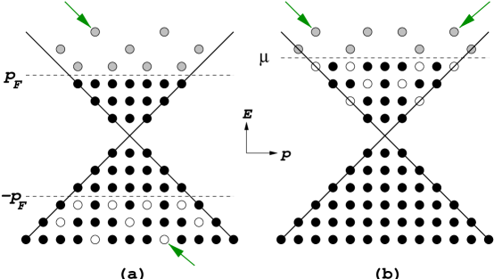
FIG. 13.: The figure shows a comparison of quark–antiquark (a) and quark–quark pairing (b). Arrows indicate typical pairs, having net zero momentum.

As in the case of ordinary BCS superconductivity in electron systems, an arbitrarily weak attractive interaction between quarks renders the quark Fermi surface unstable and leads to the formation of a condensate. Since pairs of quarks cannot be color singlets, a diquark condensate breaks color symmetry. It was originally suggested by Bailin and Love [4] (see also [84]) that QCD at very high density behaves as a “color superconductor”: Cooper pairs of quarks condense in an attractive channel opening up a gap at the Fermi surface. Recent mean field analyses of NJL–type models indicate that quark pair condensation does indeed occur and that the gaps are phenomenologically significant (of order $100$ MeV) at densities of about a few times nuclear matter density [5]. Different attractive channels may lead to a possible (simultaneous) formation of condensates. In particular, the vacuum of QCD already has a condensate of a quark–anti-quark pair. An important ingredient for the understanding of the high density phase structure is the notion of competing condensates. One expects, that the breaking of color symmetry due to a $\langle\psi\psi\rangle$ condensate is suppressed by the presence of a chiral condensate. Likewise, chiral symmetry restoration may be induced at lower densities by the presence of a color superconductor condensate. This behavior has been demonstrated explicitly within an NJL–type model and led to a first model calculation of the phase diagram [6], similar to the one sketched in the figure of section I. At low temperatures, chiral symmetry restoration occurs via a first order transition between a phase with low (or zero) baryon density and a high density color superconducting phase[6, 85, 86]. Color superconductivity is found in the high density phase for temperatures less than of order tens to 100 MeV. The strong competition between chiral and superconducting condensates also simplifies the discussion: The behavior of the chiral condensate within the low density phase is well described without taking into account diquark condensation once the phase boundary is known. We implicitly exploited this fact in section V D.

A systematic calculation in perturbation theory is only possible at asymptotically high densities, where the strong gauge coupling at the Fermi energy is small. The corresponding renomalization of quark operators in the vicinity of the Fermi surface has been studied in [87]. The method using nonperturbative flow equations, which were discussed in these lectures, may help to give some insight about these questions at lower densities. Since this remains to be done I will content myself here with some general aspects and an outlook.

The explicit form of the favored diquark condensate crucially determines the symmetry properties of the ground state at high density. Diquark operators have the structure

$$\psi^{T}\Sigma_{\rm Dirac}\Sigma_{\rm Color}\Sigma_{\rm Flavor}\psi$$ (126)

where the combination of Dirac, color and flavor matrices have to be antisymmetric according to the Pauli principle. It is instructive to do some classification. Let us divide matrices in symmetric and anti–symmetric ones, where we consider the case of vanishing angular momentum

$$\Sigma_{\rm Dirac}^{\rm A} = \bigg{\{}C\gamma_{5},C,C\gamma_{\mu}\gamma_{5}\bigg{\}}\vspace{.2cm}$$ (127)

$$\Sigma_{\rm Dirac}^{\rm S} = \bigg{\{}C\gamma_{\mu},C\sigma_{\mu\nu}\bigg{\}}\vspace{.2cm}$$ (128)

$$\Sigma_{\rm color}^{\rm A} = \bigg{\{}\lambda_{7},-\lambda_{5},\lambda_{2}\bigg{\}}\equiv\bigg{\{}\lambda^{\rm A}_{i=1,2,3}\bigg{\}}\;;\qquad(\lambda^{\rm A}_{i})_{jk}=-i\epsilon_{ijk}\vspace{.2cm}$$ (129)

$$\Sigma_{\rm color}^{\rm S} = \bigg{\{}\lambda_{0}\equiv\sqrt{\frac{2}{3}}{\bf 1},\lambda_{3},\lambda_{8},\lambda_{1},\lambda_{4},\lambda_{6}\bigg{\}}\equiv\bigg{\{}\lambda^{\rm S}_{i=1,\dots,6}\bigg{\}}\vspace{.2cm}$$ (130)

$$\Sigma_{\rm flavor}^{\rm A} = \bigg{\{}\tau_{2}\bigg{\}}\;;\qquad(\tau_{2})_{ij}=-i\epsilon_{ij}\vspace{.2cm}$$ (131)

$$\Sigma_{\rm flavor}^{\rm S} = \bigg{\{}\tau_{0}\equiv\frac{1}{2}\,{\bf 1},\tau_{1},\tau_{3}\bigg{\}}=\bigg{\{}\tau_{i=1,2,3}^{\rm S}\bigg{\}}$$ (132)

Here “A” and “S” denotes antisymmetric and symmetric, respectively; the $\tau$’s are the Pauli matrices; $C$ is the charge conjugation matrix, $\Sigma_{\rm color}^{\rm A}$ are the three antisymmetric and $\Sigma_{\rm color}^{\rm S}$ the six symmetric Gell–Mann matrices. This split corresponds to the fact that the two quarks can be comined to form a color antitriplet and a symmetric color ${\bf 6}$: $\,{\bf 3}_{c}\otimes{\bf 3}_{c}=\bar{\bf 3}_{c}+{\bf 6}_{c}$. Consider first the color ${\bf\overline{3}}$ representation. Overall antisymmetry then requires that combined Dirac–flavor has to be symmetric. If we consider the antisymmetric flavor singlet $\tau_{2}$ then the Dirac matrices must be either $C\gamma_{5}$, corresponding to a Lorentz scalar condensate, or $C$ which is a pseudoscalar. The other possible combination involving $C\gamma_{\mu}\gamma_{5}$ does not pair states near the Fermi surface and is suppressed. Instead it realizes pairing of a state near the Fermi surface and one much below with net zero momentum.

Let us turn to the question if there is indeed an attractive channel between quarks of different color. We may content ourselves here by looking at the signs for the scalar channels in the effective four quark interaction ${\cal M}$ (30)

$${\cal M}(p_{1},p_{2},p_{3},p_{4})=\displaystyle{-\left\{\bar{\psi}^{i}_{a}(-p_{1})\gamma^{\mu}\left(\frac{\lambda_{z}}{2}\right)_{i}^{\ j}\psi_{j}^{a}(-p_{3})\right\}\left\{\bar{\psi}^{k}_{b}(p_{4})\gamma_{\mu}\left(\frac{\lambda_{z}}{2}\right)_{k}^{\ \ell}\psi_{\ell}^{b}(p_{2})\right\}}\;.$$ (133)

The curled brackets indicate contractions over spinor indices, $i,j,k,l=1,2,3$ are the colour indices and $a,b=1,2$ the flavour indices of the quarks. Let us neglect for a moment the color and flavor structure of the interaction. Using the identity

$$(\gamma^{\mu})_{\alpha\beta}(\gamma_{\mu})_{\gamma\delta} = -(iC)_{\alpha\gamma}(iC)_{\delta\beta}-(\gamma^{5}C)_{\alpha\gamma}(C\gamma^{5})_{\delta\beta}\vspace{.2cm}$$ (135)

$$+\frac{1}{2}(i\gamma^{\mu}C)_{\alpha\gamma}(iC\gamma_{\mu})_{\delta\beta}-\frac{1}{2}(\gamma^{5}\gamma^{\mu}C)_{\alpha\gamma}(C\gamma^{5}\gamma_{\mu})_{\delta\beta}$$

we can rewrite the interaction in terms of quark and antiquark bilinears, respectively

$${\cal M}(p_{1},p_{2},p_{3},p_{4}) = +\left\{\bar{\psi}(-p_{1})iC\bar{\psi}^{T}(p_{4})\right\}\left\{\psi^{T}(p_{2})iC\psi(-p_{3})\right\}\vspace{.2cm}$$ (139)

$$+\left\{\bar{\psi}(-p_{1})\gamma^{5}C\bar{\psi}^{T}(p_{4})\right\}\left\{\psi^{T}(p_{2})C\gamma^{5}\psi(-p_{3})\right\}\vspace{.2cm}$$

$$-\left\{\bar{\psi}(-p_{1})i\gamma^{\mu}C\bar{\psi}^{T}(p_{4})\right\}\left\{\psi^{T}(p_{2})iC\gamma_{\mu}\psi(-p_{3})\right\}\vspace{.2cm}$$

$$+\left\{\bar{\psi}(-p_{1})\gamma^{5}\gamma^{\mu}C\bar{\psi}^{T}(p_{4})\right\}\left\{\psi^{T}(p_{2})C\gamma^{5}\gamma_{\mu}\psi(-p_{3})\right\}\;.$$

From the signs in (139) one may expect repulsion in the pseudoscalar and scalar diquark channels (compare also with the attractive scalar and pseudoscalar meson channels in (34)). However, we neglected color and flavor so far. The appropriate Fierz identity for color manifests the separation in antitriplet and color $\bf{6}$ diquark channels

$$\sum\limits_{z=1}^{8}\left(\frac{\lambda_{z}}{2}\right)_{i}^{\ j}\left(\frac{\lambda_{z}}{2}\right)_{k}^{\ \ell}=-\frac{4}{3}\sum\limits_{z=1}^{3}\left(\frac{\lambda_{z}^{\rm A}}{2}\right)_{i}^{\ k}\left(\frac{\lambda_{z}^{\rm A}}{2}\right)_{\ell}^{\ j}+\frac{2}{3}\sum\limits_{z=1}^{6}\left(\frac{\lambda_{z}^{\rm S}}{2}\right)_{i}^{\ k}\left(\frac{\lambda_{z}^{\rm S}}{2}\right)_{\ell}^{\ j}\;.$$ (140)

For flavor we use

$$\delta_{ab}\delta_{cd}=\frac{1}{2}(\tau_{2})_{ac}(\tau_{2})_{db}+\sum\limits_{z=1}^{3}(\tau_{z}^{\rm S})_{ac}(\tau_{z}^{\rm S})_{db}\;.$$ (141)

From the different relative sign for the $\bf{3}_{c}$ and the $\bf{6}_{c}$ channels in (140) we conclude that one may expect condensation in the color antitriplet Lorentz scalar and pseudoscalar channels. The corresponding color symmetric channels may not be expected to condense.

We note, however, that the four quark interaction (29) (“dressed one gluon exchange”) does not break the axial $U(1)_{A}$ of QCD. It has been shown [25] that the instanton induced interaction between light quarks properly reflects the chiral symmetry of QCD: axial baryon number is broken, while chiral $SU(2)_{L}\times SU(2)_{R}$ is respected. (The corresponding $U(1)_{A}$–breaking term can be written as a determinant (59) which has been taken into account in the effective quark meson model in section III.) Here we only note that the instanton induced interaction leads to an attractive scalar diquark channel but exhibits repulsion in the pseudoscalar channel for $\bf{3}_{c}$ [5, 6]. For two flavors triplet pairing of the form

$$\langle\psi^{i}_{a}(p)C\gamma_{5}\psi^{j}_{b}(-p)\rangle~{}=~{}\kappa(p^{2})\epsilon^{ij\ell}\epsilon_{ab}$$ (142)

has been demonstrated to lead to significant gaps of the order $100$ MeV for instanton induced interactions [5, 6]. For a nonzero expectation value of (142) the diquark bilinear has a color index $\ell$ which chooses a direction in color space, say $\ell=3$, thus breaking color symmetry $SU(3)\rightarrow SU(2)$. It leaves all flavor symmetries and, in particular, the chiral $SU(2)_{L}\times SU(2)_{R}$ intact. One may expect it to be especially favorable because it maintains a large symmetry, so that the interaction of a given pair can obtain contributions from other pairs with different particle combinations. The above pairing does not involve quarks of the third color. It is possible that the remaining ungapped Fermi surface becomes unstable too, which is of course color symmetric. An additional condensation of the form

$$\langle\psi^{3}_{a}(p)C\sigma_{0i}\psi^{3}_{b}(-p)\rangle=\eta(p^{2}){\hat{p}}_{i}\delta_{ab}$$ (143)

has been investigated [5]. This condensate violates rotation symmetry and the gaps were found to be of order several keV at best.

Breaking of the color $SU(3)$ symmetry generates Goldstone bosons, formally. However, since color is a gauge symmetry and the Higgs mechanism operates, the spectrum does not contain massless scalars but massive vectors. The number of broken generators is $8-3=5$ for condensation of the form (142) and, therefore, five gluons become massive. We have decribed here the color superconducting phase as a Higgs phase. One expects, however, that there is a complementary description in which this is a confining phase. Indeed, the color superconducting phase for two flavors may be considered as a realization of confinement without chiral symmetry breaking.

The $U(1)_{Q}$ of electromagnetism is also spontaneously broken by the condensate. However, the photon mixes with the eighth component of the gluon to generate an unbroken $U(1)_{Q^{\prime}}$. Let $T_{3}$ denotes the diagonal generator of isospin $SU(2)$ and $B$ baryon number then $Q=T_{3}+B/2$. For a nonvanishing color antitriplet condensate (142) $\Delta\sim\epsilon^{ij3}$ one finds

$$B\,\Delta=\frac{2}{3}\Delta\,\;,\quad Q\,\Delta=\frac{1}{3}\Delta\,\;,\quad\lambda_{8}\,\Delta=\frac{2}{\sqrt{3}}\Delta$$ (144)

and one observes a linear combination of electric charge and color hypercharge $Y\equiv\lambda_{8}/\sqrt{3}$ under which the condensate is neutral: $Q^{\prime}=Q-Y/2$, so a modified $U(1)$ persists. (Instead, one may also want to refer to baryon number and finds the combination $B^{\prime}=B-Y$ which leaves the condensate invariant.)

Three quark flavors. The situation is further complicated by the question about the number of light quark flavors participating in the condensate. If the strange quark were heavy relative to fundamental QCD scales, the idealization of assuming two light flavors would be obviously sufficient. The situation becomes more involved since we are interested in densities above the transition for which the chiral condensate vanishes. Without spontaneous chiral symmetry breaking the relevant strange quark is of the order $100$ MeV. Since we are interested in chemical potentials larger than $100$ MeV it is a quantitative question if an approximation with two light flavors is realistic.

In the limit of three massless quark flavors a very interesting and compelling possibility for condensation has been proposed by Alford, Rajagopal and Wilczek [7]. Consider a generalization of the two flavor condensate (142) where the antisymmetric flavor singlet $\sim\epsilon_{ab}$ is replaced by the antisymmetric triplet for three flavors $\sim\epsilon_{abc}$ Since there are an equal number of flavors and colors there is the possibility for a color–flavor structure $\sim~{}\epsilon^{ijz}\epsilon_{abz}=\delta^{i}_{a}\delta^{j}_{b}-\delta^{i}_{b}\delta^{j}_{a}$ by summing over $z$. In [7] a slightly more general variant

$$\langle\psi^{i}_{a}(p)C\gamma_{5}\psi^{j}_{b}(-p)\rangle~{}=~{}\kappa_{1}(p^{2})\delta^{i}_{a}\delta^{j}_{b}+\kappa_{2}(p^{2})\delta^{i}_{b}\delta^{j}_{a}$$ (145)

has been investigated. The mixed Kronecker matrices are invariant only under matched vectorial color/flavor rotations. Ignoring electromagnetism the symmetry of QCD with three massless flavors is $SU(3)_{\rm color}\times SU(3)_{L}\times SU(3)_{R}\times U_{B}(1)$ (cf. section II A). The $SU(3)_{\rm color}$ is a local gauge symmetry while the chiral flavor symmetry is global, as is the $U(1)_{B}$ for baryon number. As a consequence of the above matching between color and flavor symmetries for a nonvanishing condensate the only remaining symmetry is the global diagonal $SU(3)_{{\rm color}+L+R}$ subgroup. In particular, the gauged color symmetries and the global axial flavor symmetries are spontaneously broken. The latter means that chiral symmetry is broken by a new mechanism. The breaking of the $U(1)_{B}$ of baryon number leads to superfluidity as in liquid helium. All fermions aquire a gap and there are Goldstone modes associated with the spontaneous chiral symmetry breaking. The high density phase may therefore be in many ways quite similar to low density QCD [8]!

It is not clear what phase will be realized with physical mass $u$, $d$ and $s$ quarks. As pointed out in [88], one may think of having the two flavor condensate first and color–flavor locking at higher density. A first investigation may be performed along the lines presented in [6] where simultaneous condensation phenomena have been discussed, but finally more sophisticated methods than the mean field analysis will be needed to settle these questions. An interesting possibility will be the use of truncated nonperturbative flow equations along the lines presented in these lectures.

- [1]
- [2] D.J. Gross and F.A. Wilczek, Phys. Rev. Lett. 30 (1973) 1343; H.D. Politzer, Phys. Rev. Lett. 30 (1973) 1346.
- [3] J.C. Collins and M.J. Perry, Phys. Rev. Lett. 34 (1975) 1353.
- [4] D. Bailin and A. Love, Phys. Rept. 107 (1984) 325.
- [5] M. Alford, K. Rajagopal and F. Wilczek, Phys. Lett. 422B (1998) 247; R. Rapp, T. Schäfer, E.V. Shuryak and M. Velkovsky, Phys. Rev. Lett. 81 (1998) 53.
- [6] J. Berges and K. Rajagopal, Nucl. Phys. B 538 (1999) 215.
- [7] M. Alford, K. Rajagopal and F. Wilczek, Nucl. Phys. B 537 (1999) 443.
- [8] T. Schäfer and F. Wilczek, hep-ph/9811473.
- [9] S.A. Bass, M. Gyulassy, H. Stocker, W. Greiner, hep-ph/9810281.
- [10] R.D. Pisarski and F. Wilczek, Phys. Rev. D29 (1984) 338.
- [11] K. Rajagopal and F. Wilczek, Nucl. Phys. B399 (1993) 395; B404 (1993) 577.
- [12] K. Rajagopal, in Quark-Gluon Plasma 2, edited by R. Hwa (World Scientific, 1995) (hep-ph/9504310).
- [13] M.A. Halasz, A.D. Jackson, R.E. Shrock, M.A. Stephanov and J.J.M. Verbaarschot, Phys. Rev. D58 (1998) 096007.
- [14] M. Stephanov, K. Rajagopal and E. Shuryak, Phys. Rev. Lett. 81 (1998) 4816.
- [15] L. Csernai and J. Kapusta, Phys. Rep. 131 (1986) 223.
- [16] EMU01-Collaboration, hep-ph/9809289.
- [17] C. Wetterich, Phys. Lett. 301B (1993) 90.
- [18] J. Berges, D. Jungnickel and C. Wetterich, Phys. Rev. D59 (1999) 034010.
- [19] J. Berges, N. Tetradis and C. Wetterich, Phys. Rev. Lett. 77 (1996) 873.
- [20] D.-U. Jungnickel and C. Wetterich, Phys. Rev. D53 (1996) 5142.
- [21] J. Berges, D.-U. Jungnickel and C. Wetterich, hep-ph/9811347.
- [22] M. Schmelling, published in ICHEP 96, 91, hep-ex/9701002.
- [23] J. Gasser and H. Leutwyler, Phys. Rep. C87 (1982) 77.
- [24] C.P. Burgess, Lectures given at 11th Summer School and Symposium on Nuclear Physics (NuSS 98): Effective Theories of Matter (1), Seoul, Korea, 23-27 Jun 1998, hep-th/9808176.
- [25] G. ’t Hooft, Phys. Rep. 142 (1986) 357.
- [26] L.P. Kadanoff, Physica 2 (1966) 263.
- [27] K.G. Wilson, Phys. Rev. B4 (1971) 3174; K.G. Wilson and I.G. Kogut, Phys. Rep. 12 (1974) 75.
- [28] C. Wetterich, Nucl. Phys. B352 (1991) 529; Z. Phys. C57 (1993) 451; C60 (1993) 461.
- [29] C. Wetterich, Z. Phys. C48 (1990) 693; S. Bornholdt and C. Wetterich, Z. Phys. C58 (1993) 585.
- [30] M. Reuter and C. Wetterich, Nucl. Phys. B391 (1993) 147.
- [31] C. Becchi, preprint GEF-TH-96-11 (hep-th/9607188).
- [32] M. Bonini, M. D’ Attanasio and G. Marchesini, Nucl. Phys. B418 (1994) 81.
- [33] U. Ellwanger, Phys. Lett. 335B (1994) 364: U. Ellwanger, M. Hirsch and A. Weber, Z. Phys. C69 (1996) 687.
- [34] G. Keller, C. Kopper and M. Salmhofer, Helv. Phys. Acta 65 (1992) 32; G. Keller and G. Kopper, Phys. Lett. B273 (1991) 323.
- [35] F. Wegner and A. Houghton, Phys. Rev. A8 (1973) 401; F. Wegner, in Phase Transitions and Critical Phenomena, vol. 6, eds. C. Domb and M.S. Greene (Academic Press, 1976).
- [36] J.F. Nicoll and T.S. Chang, Phys. Lett. A62 (1977) 287.
- [37] S. Weinberg in Critical Phenomena for Field Theorists, Erice Subnucl. Phys. (1976) 1;
- [38] J. Polchinski, Nucl. Phys. B231 (1984) 269.
- [39] A. Hasenfratz and P. Hasenfratz, Nucl. Phys. B270 (1986) 687; P. Hasenfratz and J. Nager, Z. Phys. C 37 (1988) 477.
- [40] M. Bonini, M. D’ Attanasio and G. Marchesini, Nucl. Phys. B409 (1993) 441.
- [41] U. Ellwanger, Z. Phys. C58 (1993) 619; C. Wetterich, Int. J. Mod. Phys. A9 (1994) 3571.
- [42] C. Kim, Lectures given at 11th Summer School and Symposium on Nuclear Physics (NuSS 98): Effective Theories of Matter (1), Seoul, Korea, 23-27 Jun 1998, hep-th/9810056.
- [43] J. Comellas, Y. Kubyshin and E. Moreno, Nucl. Phys. B490 (1997) 653.
- [44] M. LeBellac, Quantum and Statistical Field Theory, Oxford Science Publications, 1994.
- [45] D.–U. Jungnickel and C. Wetterich, Lectures given at the NATO Advanced Study Institute on Confinement, Duality and Nonperturbative Aspects of QCD, Cambridge, England, 23 Jun - 4 Jul 1997, hep-ph/9710397.
- [46] C. Wetterich, Z. Phys. C 72 (1996) 139.
- [47] B. Bergerhoff and C. Wetterich, Phys. Rev. D57 (1998) 1591.
- [48] U. Ellwanger, M. Hirsch and A. Weber, Eur. Phys. J. C1 (1998) 563.
- [49] U. Ellwanger and C. Wetterich, Nucl. Phys. B423 (1994) 137.
- [50] Y. Nambu and G. Jona–Lasinio, Phys. Rev. 122 (1961) 345; V. G. Vaks and A. I. Larkin, Sov. Phys. JETP 13 (1961) 192.
- [51] J. Bijnens, Phys. Rep. 265 (1996) 369.
- [52] S. P. Klevansky, Rev. Mod. Phys. 64 (1992) 649.
- [53] M. Gell–Mann and M. Levy, Nuovo Cim. 16 (1960) 705.
- [54] J. Pawlowski, Phys. Rev. D58 (1998) 045011.
- [55] J. Kapusta, Finite Temperature Field Theory (Cambridge University Press, 1989).
- [56] N. Tetradis and C. Wetterich, Nucl. Phys. B398 (1993) 659; Int. J. Mod. Phys. A9 (1994) 4029.
- [57] For a review see H. Meyer–Ortmanns, Rev. Mod. Phys. 68 (1996) 473.
- [58] A. Barducci, R. Casalbuoni, S. De Curtis, R. Gatto and G. Pettini, Phys. Lett. B231 (1989) 463.
- [59] S. Gavin, A. Gocksch and R. Pisarski, Phys. Rev. D49 (1994) 3079.
- [60] E. Shuryak, Comm. Nucl. Part. Phys. 21 (1994) 235.
- [61] M. Reuter and C. Wetterich, Nucl. Phys. B408 (1993) 91, 417 (1994) 181, 427 (1994) 291.
- [62] N. Tetradis and C. Wetterich, Nucl. Phys. B422 (1994) 541.
- [63] J. Adams, J. Berges, S. Bornholdt, F. Freire, N. Tetradis and C. Wetterich, Mod. Phys. Lett. A10 (1995) 2367.
- [64] J. Berges, Field Theory near the Critical Temperature, Erice Subnucl. Phys., 34th Course, Effective Theories and Fundamental Interactions (1996), 504, hep-ph/9610353.
- [65] B. Widom, J. Chem. Phys. 43 (1965) 3898.
- [66] D. Toussaint, Phys. Rev. D55 (1997) 362.
- [67] E. Brezin, D.J. Wallace and K.G. Wilson, Phys. Rev. B7 (1973) 232.
- [68] G. Baker, D. Meiron and B. Nickel, Phys. Rev. B17 (1978) 1365.
- [69] K. Kanaya and S. Kaya, Phys. Rev. D51 (1995) 2404.
- [70] J. Zinn-Justin, Quantum Field Theory and Critical Phenomena (Oxford University Press, 1993).
- [71] T.R. Morris and M.D. Turner, Nucl. Phys. B509 (1998) 637.
- [72] C. Bernard et al., Phys. Rev. D55 (1997) 6861; C. Bernard et al., Nucl. Phys. Proc. Suppl. 53 (1997) 442.
- [73] For a review see E. Laermann, Nucl. Phys. Proc. Suppl. 63 (1998) 114 and references therein.
- [74] D.–U. Jungnickel and C. Wetterich, Phys. Lett. B389 (1996) 600.
- [75] D.–U. Jungnickel and C. Wetterich, Eur. Phys. J. C2 (1998) 557.
- [76] J. Gasser and H. Leutwyler, Phys. Lett. B184 (1987) 83; H. Leutwyler, Nucl. Phys. Proc. Suppl. B4 (1988) 248.
- [77] D.–U. Jungnickel and C. Wetterich, Eur. Phys. J. C1 (1998) 669.
- [78] I. M. Barbour, S. E. Morrison, E. G. Klepfish, J. B. Kogut, Maria-Paola Lombardo, Nucl. Phys. Proc. Suppl. 60A (1998) 220.
- [79] S. Hsu and M. Schwetz, Phys. Lett. B432 (1998) 203.
- [80] J. Berges, D.-U. Jungnickel and C. Wetterich, hep-ph/9811387.
- [81] G. Benfatto and G. Galavotti, Renormalization Group, Princeton University Press, Princeton, 1995; R. Shankar, Rev. Mod. Phys. 66, (1993) 129; J. Polchinski, Lectures presented at TASI 92, Boulder, CO, June 3–28, 1992 hep-th/9210046.
- [82] I. Lawrie and S. Sarbach in Phase Transitions and Critical Phenomena 9 (1984) 1, ed. C. Domb and J. Lebowitz (Academic Press).
- [83] M. Alford, hep-lat/9809166.
- [84] B. Barrois, Nucl. Phys. B 129 (1977) 390, and Caltech doctoral thesis (1978), unpublished.
- [85] J. Berges, QCD at High Baryon Density and Temperature: Competing Condensates and the Tricritical Point, Workshop on QCD at Finite Baryon Density, Bielefeld, Germany, 27-30 April 1998, Nucl. Phys. A642 (1998) 51.
- [86] G.W. Carter and D. Diakonov, hep-ph/9812445.
- [87] N. Evans, S.D.H. Hsu and M. Schwetz, hep-ph/9808444; hep-ph/9810514; T. Schäfer and F. Wilczek, hep-ph/9810509; D. T. Son, hep-ph/9812287.
- [88] E. Shuryak, Nucl. Phys. A642 (1998) 14.