Unitarized Diffractive Scattering in QCD
and Application to Virtual Photon Total Cross Sections

Abstract

The problem of restoring Froissart bound to the BFKL-Pomeron is studied in an extended leading-log approximation of QCD. We consider parton-parton scattering amplitude and show that the sum of all Feynman-diagram contributions can be written in an eikonal form. In this form dynamics is determined by the phase shift, and subleading-logs of all orders needed to restore the Froissart bound are automatically provided. The main technical difficulty is to find a way to extract these subleading contributions without having to compute each Feynman diagram beyond the leading order. We solve that problem by using nonabelian cut diagrams introduced elsewhere. They can be considered as colour filters used to isolate the multi-Reggeon contributions that supply these subleading-log terms. Illustration of the formalism is given for amplitudes and phase shifts up to three loops. For diffractive scattering, only phase shifts governed by one and two Reggeon exchanges are needed. They can be computed from the leading-log-Reggeon and the BFKL-Pomeron amplitudes. In applications, we argue that the dependence of the energy-growth exponent on virtuality $Q^{2}$ for $\gamma^{*}P$ total cross section observed at HERA can be interpreted as the first sign of a slowdown of energy growth towards satisfying the Froissart bound. An attempt to understand these exponents with the present formalism is discussed.

I Introduction

Large rapidity-gap events observed recently at HERA [1, 2] provide additional impetus to QCD calculation of diffractive scattering and total cross section. At virtuality $Q^{2}\gg\Lambda_{QCD}^{2}$, the QCD fine structure constant $\alpha_{s}=g^{2}/4\pi$ is small, near-forward parton-parton scattering is in principle calculable in perturbation theory, and total cross section can be obtained via the optical theorem. To be sure, such calculation is very complicated at high c.m. energy $\sqrt{s}$, as the effective expansion parameter for the problem is $\alpha_{s}\ln s$ and not just $\alpha_{s}$. The former could be large at high $s$ even though the latter may be small. As a result, multi-loop diagrams must be included.

To make multi-loop calculations feasible, leading-log approximation (LLA) is usually employed. This consists of keeping only the highest power of $\ln s$ at each order. Equivalently, if the scattering amplitude (divided by $s$) is considered as a function of the two variables $\alpha_{s}$ and $\alpha_{s}\ln s$, then only the lowest power of $\alpha_{s}$ is kept. When the resulting amplitude is of the form $\alpha_{s}^{n}sF(\alpha_{s}\ln s)$ for some function $F$, we will abbreviate it simply as $\sim\hskip-3.0pt\alpha_{s}^{n}$.

The LLA result for high-energy near-forward scattering is known, though not completely. The dominant parton-parton scattering amplitude occurs with the exchange of a colour-octet object called the Reggeon (or the Reggeized gluon), and is $\sim\hskip-3.0pt\alpha_{s}$ [3]. The Reggeon amplitude is actually proportional to $(\alpha_{s}s/\Delta^{2})s^{R(\Delta)}$, with $\Delta^{2}=-t$ the square of the momentum transfer, and $R(\Delta)$ a known function of $\Delta$ proportional to $\alpha_{s}$. Note that $s^{R(\Delta)}$ is of the form $F(\alpha_{s}\ln s)$, so the Reggeon amplitude is indeed $\sim\hskip-3.0pt\alpha_{s}$, as claimed. Although the Reggeon amplitude is the dominant result for summing all diagrams in LLA, it can be obtained just from the $t$-channel ladder diagrams and their gauge partners, because all the other diagrams are subdominant. We may therefore think of the Reggeon as a composite object made up of gluons, bundled up together roughly in a ladder configuration.

Diffractive scattering occurs via a colour-singlet exchange. Two or more Reggeons are required to form a colour-singlet object in the $t$ channel. Since each Reggeon carries a small factor $\sim\hskip-3.0pt\alpha_{s}$, the dominant singlet amplitude comes from two interacting Reggeons, giving a magnitude $\sim\hskip-3.0pt\alpha_{s}^{2}$. This is the BFKL Pomeron [3, 4]. Unfortunately this amplitude is not known too precisely, though one does know that in the forward direction and extremely high energies it behaves like $s^{J}$, with $J>1$ a known number. This gives rise to a total cross section with energy variation $s^{J-1}$, which violates the Froissart bound $(\ln s)^{2}$.

Present data from HERA [1, 2] on $\gamma^{*}P$ total cross section are consistent with a power growth in $s$, though with an observed exponent smaller than $J-1$ computed from the BFKL Pomeron. To satisfy unitarity and obey the Froissart bound, the exponent must eventually decrease to zero at very high energies, and that can be achieved theoretically only by including subleading-log contributions that have been hitherto neglected. The first subleading correction to the BFKL Pomeron have been computed [5], with the encouraging result of a smaller $J$, but also with a pathological behaviour that has not yet been fully resolved. In any case the Froissart bound is still violated.

From the $s$-channel unitarity relation 2Im$(T_{fi})=\sum_{n}T^{*}_{fn}T_{ni}$, one expects all multiple-Reggeon exchanges to have to be included before we can restore full unitarity and the Froissart bound. As each additional Reggeon brings in an extra factor of $\sim\hskip-3.0pt\alpha_{s}$, they provide the required subleading-log contributions to all orders. The purpose of this paper is to discuss a formalism whereby this scenario can be implemented in pQCD. For other approaches see for example [6].

To clarify what we have in mind, let us first pretend the partons to be scattered through a two-body instantaneous potential $V(\vec{x})$. Born amplitude alone violates unitarity, but that can be fixed up by including all higher-order corrections. For small $V$, these higher-order terms are the analogs of the subleading contributions discussed above. These amplitudes can be summed up at high energy into an eikonal formula (see eq. (1)) [7] where unitarity is restored. Dynamics is now specified by the phase shift $\delta(b)$, which is a function of the impact parameter $b$, and is linear in $V$. Higher-order amplitudes can be recovered by expanding the exponential into powers of the phase shift.

A very similar scenario emerged if the two partons interacted through a multiple exchange of photons. In that case the interaction is no longer instantaneous, and cross diagrams are present. In terms of the unitarity relation, this means photons are present in the intermediate states and the inelastic channels in which they are produced must be included in the unitarity sum. However, the eikonal form can still be established with the help of the ‘eikonal formula’ [8], and the phase shift is still given by the Born approximation amplitude (the Coulomb phase shift) [9, 10].

There is nothing new about using the eikonal form to implement unitarity. In fact, a very large amount of phenomenology of two-body scattering has been carried out in that framework. The modern challenge is whether, and if so how, pQCD amplitudes can be unitarized that way. For on-shell near-forward hadronic scatterings, confinement is presumably important and we may not even be able to use pQCD. However, $\gamma^{*}P$ total cross section at large virtuality is expected to be calculable in pQCD, and the BFKL Pomeron is an attempt to do so. Unfortunately it violates the Froissart bound, so the implementation of unitarity in pQCD remains unsolved. This is the area where we hope to make some progress on. The main difficulty comes from the fact that terms with all powers of $\alpha_{s}$ (with fixed $\alpha_{s}\ln s$) are needed to restore unitarity, but these are small terms extremely difficult to obtain from Feynman diagrams in the calculable regime $\alpha_{s}\ll 1$.

The following physical picture [11] may help to visualize how the Froissart bound is restored. The rise of total cross section [13] predicted by the BFKL Pomeron [4] may be attributed to an increased production of gluon jets at higher energies. When the energy gets really high, there are so many gluons around that they tend to overlap one another. When that happens, coherent effect becomes important and a destructive interference sets in to reduce the power growth, to a rate that eventually satisfies the Froissart bound $(\ln s)^{2}$. This mechanism suggests that whatever formalism we use to restore the Froissart bound, interference effects ought to be a central part of it. The ‘nonabelian cut diagrams’ we propose to use to solve this problem fits into this category, because they can be viewed as a way to organize the summation of Feynman diagrams to heighten the Bose-Einstein interference effects of identical gluons [14].

Returning to the formal mechanism to unitarize QCD, the first thought would be to try to imitate potential scattering and QED by including multiple exchanges of Reggeons and/or Pomerons. This is indeed the general idea but there are non-trivial problems to be solved with this approach. Unlike the photon in QED or the potential, Reggeon and Pomeron are composite objects, themselves made up of gluons and possibly quark pairs. It is therefore not clear whether we are allowed to exchange them as if they were elementary. For example, should we include diagrams where Reggeons are crossed? Or equivalently, can Reggeons be produced from the partons so that inelastic channels involving their production must be included in the unitarity sum like QED? Can these composite objects overlap and merge? If an effective theory of Reggeon/Pomeron equivalent to QCD existed without gluons, then presumably we would be able to answer all these questions once its precise dynamics is known. However, since gluons can be produced off Reggeons and Pomerons, they must be included in any effective theory [12], in which case it is hard to exclude them from being exchanged as well. If we have to exchange gluons anyhow, we might as well go back to the original QCD theory which exchanges nothing but gluons and quarks, and whose dynamics is precisely known. At least we can avoid potential double counting if we do it that way. Nevertheless, gluon self-interaction and non-commutativity of colour matrices have no analog in the potential or the QED problem, so it is not clear how the very complicated QCD Feynman diagrams can be handled. It is even less certain that the results can be mimicked by the exchange of Reggeons and/or Pomerons which we hope to see. Worst of all, Feynman diagrams can hardly be calculated beyond LLA, but we need subleading contributions to build up the eikonal form and unitarity. How can we possibly get them without going through the impossible task of computing Feynman diagrams to highly subleading orders?

Fortunately these questions can be answered and difficulties overcome, if we use the nonabelian cut diagrams introduced elsewhere [15, 16, 17, 18] instead of the conventional Feynman diagrams. Reggeons and Pomerons emerge naturally, and phase shifts can be calculated using only the leading-log approximation. Due to the possibility of gluon production from Reggeons, phase shift is generally no longer linear in the (Reggeon) exchange, as was the case in potential scattering and QED.

Nonabelian cut diagrams will be reviewed in Secs. 3 and 4. They are Feynman diagrams with slightly different ‘Feynman rules’. A permuted sum of Feynman diagrams can be shown to be equal to a permuted sum of (nonabelian) cut diagrams, which is why we may calculate amplitudes using either of them. The main advantage of cut diagram is that identification with Reggeon becomes natural. In fact, each cut amplitude is given by a product of Reggeon (fragment) amplitudes. This factorization allows the eikonal form to be built up, and subleading terms to be computed just in the leading-log approximations.

We have used the word Reggeon fragment amplitudes to mean finite-order amplitudes whose sum builds up the full Reggeon amplitude. Hence the word ‘fragment’. There may be many distinct fragments even at a given order. For brevity, the word ‘fragment’ will often be dropped.

In Sec. 2, the impact-parameter representation of a high-energy two-body amplitude is reviewed. A physical argument is given to show how the Froissart bound is restored when the bound-violating Born approximation is iterated and summed up into an eikonal form. In Sec. 3, nonabelian factorization formula [15, 16] and nonabelian cut diagrams [17, 18] for tree amplitudes are reviewed; nonabelian cut diagrams are simply Feynman diagrams with the factorization formula built in. It is important to note that this factorization has nothing to do with the usual factorization of hard physics from soft physics [9]. The present one goes along the $s$-channel, whereas the usual one goes along the $t$-channel. In Sec. 4, the technique is applied to two-body scattering amplitudes. The advantage of using cut diagram over Feynman diagram to compute a permuted sum is discussed. The connection with Reggeons is identified. The question of factorizability of these amplitudes into irreducible parts is discussed in Sec. 5. This factorization allows the eikonal form to be built up and phase shifts computed from the irreducible amplitudes. Diffractive scattering is considered in Sec. 6. In that case phase shift may be restricted to those obtained from one and two irreducible Reggeon exchanges, and can be computed from the LLA-Reggeon and BFKL-Pomeron amplitudes. By using phase shifts in the eikonal form unitarization of the diffractive amplitude is achieved. To illustrate the details of previous sections, quark-quark scattering amplitudes and phase shifts are given to the three-loop order in Sec. 7. Sec. 8 is devoted to the observed $\gamma^{*}P$ total cross sections. We argue that the dependence of the energy-growth exponent on virtuality $Q^{2}$, as well as the size of the BFKL exponent compared to the observed ones, can be taken as indications that the softening of energy growth towards the Froissart-bound limit is already happening. Correct energy dependence at various virtuality $Q^{2}$ can be reproduced with the formulae of Sec. 7. Finally, Appendix A contains some colour-algebra calculations.

II Impact-Parameter Representation, Phase Shifts,
and the Froissart Bound

Let $A(s,\Delta)$ be a parton-parton scattering amplitude at centre-of-mass energy $\sqrt{s}$ and momentum transfer $\Delta=|{\bf\Delta}|$. At high energies ${\bf\Delta}$ is transverse, and conjugate to the impact-parameter ${\bf b}$. Bold letters like ${\bf\Delta}$ and ${\bf b}$ are used to describe vectors in the transverse plane.

The two-dimensional Fourier transform of $A(s,\Delta)$ defines the impact-parameter amplitude ${\cal A}(s,b)$ by the eikonal formula

$$A(s,\Delta)=2is\int d^{2}{\bf b}e^{i{\bf\Delta}\cdot{\bf b}}{\cal A}(s,b)\equiv 2is\int d^{2}{\bf b}e^{i{\bf\Delta}\cdot{\bf b}}\left(1-e^{2i\delta(s,b)}\right).$$ (1)

For large $s\simeq 4k^{2}$, angular momentum is given by $l=kb$, and $\delta(s,b)$ is just the phase shift at that angular momentum. For QCD parton scatterings, the initial and final partons may contain different colours, so the amplitudes $A(s,\Delta)$ and ${\cal A}(s,b)$, as well as the phase shift $\delta(s,b)$, should be treated as colour matrices. Only the diagonal matrix elements arising from a colour-singlet exchange are truly elastic amplitudes. We shall denote them by $A_{1}(s,\Delta)$ and ${\cal A}_{1}(s,b)$. In terms of them, the total cross section $\sigma_{T}(s)$ is given by the optical theorem to be

$$\sigma_{T}(s)={1\over s}{\rm Im}\left[A_{1}(s,0)\right].$$ (2)

No approximation has been made to arrive at (1), so unitarity is exact and the Froissart bound is satisfied. If $\delta(s,b)$ is small, the exponential may be expanded and only the term linear in $\delta(s,b)$ kept. This gives the ‘Born amplitude’ and allows the phase shift to be thought of as the ‘potential’. Thus if the interaction causing the scattering has a range $\mu^{-1}$, then we expect $\delta(s,b)\sim\!a\exp(-\mu b)$. At large impact parameters, $a$ may be taken to be approximately independent of $b$. In the region $\mu b\gg 1$, the phase shift is small and the impact amplitude ${\cal A}(s,b)$ in (1) ceases to contribute. The effective radius $R(s)$ of interaction may therefore be estimated from the condition $\delta(s,R)\sim 1$. If $a$ is an increasing function of $s$, then $R(s)$ and hence $\sigma_{T}\sim\pi R(s)^{2}$ also increase with $s$. In particular, if $a\sim s^{J-1}$ has a power growth, caused for example by the exchange of a spin $J>1$ Pomeron or elementary particle, then $R(s)\sim[(J-1)/\mu]\ln s$, and $\sigma_{T}\sim(\ln s)^{2}$, which is the Froissart bound. This conclusion is general and is qualitatively independent of the magnitude of $J$ and the range $\mu^{-1}$. Unless $a$ increases faster than a power of $s$, the Froissart bound is guaranteed when total cross-sections are calculated from the phase shift. On the other hand, if we used the ‘Born approximation’ throughout, then the total cross section would have grown like $s^{J-1}$ all the way, and the Froissart bound would be violated. This is essentially what happens to the BFKL Pomeron [4]. The cure, very roughly speaking, is to use it as a phase shift rather than an amplitude. This is the general idea but details are more complicated. They will be discussed in Sec. 6.

To make use of this unitarization mechanism we must find a way to calculate the phase shift. This is not simple for several reasons. According to (1), even when $\delta(s,b)$ is computed just to the lowest order, the resulting $A(s,\Delta)$ contains terms of all orders. This suggests that a proper understanding of phase shifts cannot be obtained until we know how to sum an infinite number of Feynman diagrams. To put it differently, we have to learn how to deal with $2i\delta(s,b)=\ln(1-{\cal A}(s,b))$, which consists of an infinite sum of all powers of the matrix amplitude ${\cal A}(s,b)$.

Moreover, according to (1), to be successful a certain product structure must emerge out of the sum. If the phase shift is expanded in powers of the coupling constant $g^{2}$, $\delta(s,b)\simeq\sum_{m}g^{2m}\delta^{(m)}$, then the $(2n)$th order contribution to ${\cal A}(s,b)$ is given by a sum of products of the phase shifts $\delta^{(m_{i})}$, with $\sum m_{i}=n$. Individual Feynman diagrams certainly do not factorize in this manner, and it is not immediately clear why sums of Feynman diagrams have this structure either. But unless we can get the sum into this factorized form there would seem to be no simple way to extract the phase shift from Feynman diagrams.

In the next two sections we shall lay down the foundation which enables us to build up such a factorized form.

III Eikonal Approximation and Factorization of Nonabelian Tree Amplitudes

The decomposition of sums of Feynman diagrams into sums of products of Reggeon amplitudes, or of phase shifts, is based on a nonabelian factorization formula [15, 16]. This formula for tree amplitudes is the nonabelian generalization of the eikonal formula [8] used in high-energy scattering in QED. It can be conveniently embedded into Feynman diagrams to turn them into nonabelian cut diagrams [17, 18]. These items will be reviewed in the present section.

The formula deals with a sum of tree amplitudes like Fig. 1, in which a fast particle of final momentum ${p^{\prime}}^{\mu}$ emerges from an initial particle with momentum $p^{\mu}$ after the emission of $n$ gluons of momenta $k_{i}^{\mu}$. Spins and vertex factors are ignored in this section but they will be incorporated later. The gluons concerned need not be on shell. This allows the tree diagram to be a part of a much larger Feynman diagram, so that formulae developed for trees here are also useful for more complicated diagrams later. We shall assume the energy $p^{0}\simeq{p^{\prime}}^{0}$ of the fast particle to be much larger than its mass $m$, its transverse momentum $\Delta=|{\bf\Delta}|$, the square-root virtuality $Q$ in case it is present, and all the components $k_{i}^{\mu}$ of every gluon momentum; in short, larger than any other energy scale involved. It is convenient to use a somewhat unconventional system in which the final particle moves along the z-axis. In the light-cone coordinates defined by $A^{\pm}=(A^{0}\pm A^{3})$, the final four-momentum of the energetic particle can then be written as ${p^{\prime}}^{\mu}=(p^{+},p^{-},{\bf p})=(\sqrt{s},0,0)$, where terms of $o(1)$ have been dropped. The initial momentum $p^{\mu}$ of the fast particle then carries a transverse component ${\bf\Delta}=\sum_{i=1}^{n}{\bf k}_{i}$. In the eikonal approximation outlined above,

$${1\over(p^{\prime}+K)^{2}-m^{2}+i\epsilon}={1\over 2p^{\prime}\cdot K+K^{2}+i\epsilon}\simeq{1\over 2p^{\prime}\cdot K+i\epsilon}\simeq{1\over\sqrt{s}}{1\over K^{-}+i\epsilon}$$ (3)

can be made on all propagators of the fast particle, provided $K$ is the sum of any number of the $k_{i}$’s. The factor $s^{-{1\over 2}}$ in (3) is irrelevant for the rest of this section so it will be dropped and the propagators taken simply to be $(K^{-}+i\epsilon)^{-1}$.

The tree amplitude in Fig. 1 is then given by the product of a momentum factor $a[\tilde{\sigma}]$ and a colour factor $t[\tilde{\sigma}]$, where

$$a[\tilde{\sigma}] = -2\pi i\delta\left(\sum_{j=1}^{n}k^{-}_{j}\right)\prod_{i=1}^{n-1}{1\over\sum_{j=1}^{i}k^{-}_{i}+i\epsilon},$$ (4)

$$t[\tilde{\sigma}] = t_{1}t_{2}t_{3}\cdots t_{n}.$$ (5)

The $\delta$-function in $a[\tilde{\sigma}]$ is there to ensure the initial-state momentum $p=p^{\prime}+\sum_{i=1}^{n}k$ to be on shell, for in the eikonal approximation its square is $m^{2}+\sqrt{s}\sum_{i=1}^{n}k^{-}_{i}$. Since this $\delta$-function is not explicitly contained in the T-matrix, it should be removed at the end, but for the sake of a simple statement in the factorization formula (6) below it is convenient to include it in $a[\tilde{\sigma}]$ for now.

The colour factor $t[\tilde{\sigma}]$ is given by a product of $SU(N_{c})$ colour matrices $t_{a}$ in the representation appropriate to the fast particle.

Since gluons obey Bose-Einstein statistics, we must sum over all their permutations to obtain the complete tree amplitude. Let $[\sigma]=[\sigma_{1}\sigma_{2}\cdots\sigma_{n}]$ indicate the ordering of gluons along the fast particle from left to right. This symbol will also be used to denote the corresponding tree diagram. In this notation Fig. 1 corresponds to $[\sigma]=[\tilde{\sigma}]\equiv[123\cdots n]$. The tree amplitude for the diagram $[\sigma]$ will be denoted by $a[\sigma]t[\sigma]$; they are given by (5) with appropriate permutation of the gluon momenta. The complete tree amplitude is given by the sum of individual tree amplitudes over the $n!$ permutations $[\sigma]$ of the permutation group $S_{n}$. The factorization formula [15, 16] states that this permuted sum can be replaced by a similar sum of the nonabelian cut amplitudes:

$$\sum_{[\sigma]\in S_{n}}a[\sigma]t[\sigma]=\sum_{[\sigma]\in S_{n}}a[\sigma_{c}]t[\sigma_{c}^{\prime}].$$ (6)

Just like the amplitudes on the left-hand side which can be obtained from Feynman diagrams, the (nonabelian) cut amplitudes $a[\sigma_{c}]t[\sigma_{c}^{\prime}]$ on the right-hand side can be obtained from nonabelian cut diagrams[17, 18]. The (nonabelian) cut diagrams are Feynman diagrams with cuts inserted at the appropriate propagators. The ‘Feynman rules’ for cut diagrams are the usual ones except at and around the cut propagators, as we shall explain. The position of the cuts depends on $[\sigma]$, and is given by the following rule. A cut is placed just to the right of gluon $\sigma_{i}$ if and only if $\sigma_{i}<\sigma_{j}$ for all $j>i$. We shall label a cut by a vertical bar, either on the diagram itself or in the corresponding permutation symbol $[\sigma]$. The resulting nonabelian cut diagram will be denoted by $[\sigma_{c}]$. For example, if $[\sigma]=[32145]$, then $[\sigma_{c}]=[321|4|5]$. If $[\sigma]=[12354]$, then $[\sigma_{c}]=[1|2|3|54]$.

The momentum factor of a cut amplitude, $a[\sigma_{c}]$, is obtained from the momentum factor $a[\sigma]$ of the Feynman amplitude by replacing the Feynman propagator $(K^{-}+i\epsilon)^{-1}$ of every cut line by the Cutkosky propagator $-2\pi i\delta(K^{-})$. There is then a superficial similarity between a Cutkosky cut diagram and a nonabelian cut diagram. However, they are completely different and the cut diagrams referred to in this paper are exclusively nonabelian cut diagrams.

From (5), it follows that $a[\sigma_{c}]$ is factorized into products of $a$’s separated by cuts, which is why the formula is called the factorization formula. For example, if $[\sigma_{c}]=[321|4|5]$, then $a[\sigma_{c}]=a[321]a[4]a[5]$.

We mentioned below eq. (5) that the $\delta$-function appearing in the amplitude must be removed at the end. This can be carried out by putting in Cutkosky propagators only where a vertical bar occurs. The overall $\delta$-fucntion for the sum of the ‘$-$’ components of momenta then disappears because no cut is ever put after the last entry $\sigma_{n}$ of $[\sigma]=[\sigma_{1}\sigma_{2}\cdots\sigma_{n}]$.

The complementary cut diagram (or c-cut diagram for short) $[\sigma^{\prime}_{c}]$ of a cut diagram $[\sigma_{c}]$ is one in which every cut line in $[\sigma_{c}]$ becomes uncut, and vice versa. If no cuts appear in $[\sigma_{c}^{\prime}]$, the colour factor $t[\sigma_{c}^{\prime}]$ is simply the product of colour matrices, as in a Feynman diagram. When cuts are present, the product straddling an isolated cut is replaced by its commutator. If consecutive cuts occur, then the product is replaced by nested multiple commutators. For example, if $[\sigma]=[32145]$, then $[\sigma_{c}]=[321|4|5]$, $[\sigma_{c}^{\prime}]=[3|2|145]$, and $t[\sigma_{c}^{\prime}]=[t_{3},[t_{2},t_{1}]]t_{4}t_{5}$.

For $n=2$, eq. (6) reads $a[12]t[12]+a[21]t[21]=a[1|2]t[12]+a[21]t[2|1]=a[1]a[2]t_{1}t_{2}+a[21][t_{2},t_{1}]$. This can easily be checked by direct calculation. Explicit check for $n=3$ is also possible [15], but for larger $n$ a direct verification becomes very complicated.

The factorization formula (6) is combinatorial in nature, and is true whatever the matrices $t_{i}$ are. In particular, if all the matrices $t_{i}$ commute, as in QED, then the only surviving term on the right-hand side of (6) is the one where no commutator occurs, which means that $[\sigma_{c}^{\prime}]$ contains no cuts, and $[\sigma_{c}]$ has a cut at each propagator. This implies factorization of the tree amplitude (6) into a single product $\prod_{i=1}^{n}a[i]$, which is the usual eikonal formula [8, 10] used in QED scatterings. It is this factorization that allows exponentiation to occur and the phase shift to be computed.

In QCD, colour matrices do not commute,

$$[t_{a},t_{b}]=if_{abc}t_{c},$$ (7)

but their commutators generate other colour matrices. This allows the nested multiple commutator of colour matrices to be interpreted as a source for a new adjoint-colour object, which we call a Reggeon fragment. For parton-parton scattering in the weak coupling limit, they turn out to be the constituents of the Reggeon as we know it from the Regge-pole theory, hence the name. The word ‘fragment’ is there to clarify that this object is just part of the Reggeon, not the whole thing, but for brevity this word is often dropped. This algebraic characterization of a Reggeon is valid even in the strong coupling limit, or physical situations other than two-parton scatterings. Unlike a gluon which is a point-like particle, a Reggeon is an extended object made up of a bundle of gluons, each interacting with the energetic particle at a different point. Later we may also introduce interactions between gluons to tie them together. Note that there are at least as many distinct Reggeon fragments as there are nested multiple commutators. With this interpretation, the cut amplitude $a[\sigma_{c}]t[\sigma_{c}^{\prime}]$ is nothing but a product of $M$ such Reggeon amplitudes, with $M-1$ being the number of cuts in $[\sigma_{c}]$.

Two final remarks. First, the rule of inserting cuts explained above depends on how the gluons are labelled, though at the end of the calculation it should clearly not matter how it is done. We may adopt the labelling which is most convenient for our purpose. Secondly, we have assumed the fast particle to carry a large ‘+’ component of the light-cone momentum, but we may equally well construct cut diagrams if it had a large ‘$-$’ component instead. For parton-parton scattering, both are required.

IV Parton-Parton Scattering Amplitudes

We will study two-body amplitudes in this section using cut diagrams. Cut diagrams are easier to compute than the corresponding Feynman diagrams, $\ln s$ cancellations occuring in permuted sum of Feynman diagrams do not happen in this case, and they are directly related to the Reggeon (fragment) amplitudes. These are some of the advantages of using cut diagrams.

Fig. 2 depicts a QCD Feynman diagram for the scattering of two energetic partons. The upper one carries an incoming momentum $p_{1}^{\mu}=(\sqrt{s},0,{\bf 0})$ in light-cone coordinates, and the lower one carries an incoming momentum ${p_{2}}^{\mu}=(0,\sqrt{s},{\bf 0})$. Suppose there are $n_{1}$ gluons attached to the upper parton and $n_{2}$ to the lower, then the $n_{1}!n_{2}!$ diagrams obtained by permuting the position of attachment forms a permuted set of diagrams. The sum of amplitudes for diagrams in the permuted set will be called a premuted sum of amplitudes. If we replace the Feynman tree attached to each energetic parton by the corresponding cut tree, as in Sec. 3, then we have a cut diagram. According to (6), a permuted sum of Feynman amplitudes is equal to a permuted sum of cut amplitudes, which is why we may use cut diagrams instead of Feynman diagrams for computation. However, when both parton trees are permuted we may overcount, in which case the final result has to be divided by a symmetry factor ${\cal S}$. This for example will happen to a permuted sum of $s$-channel ladder diagrams. If $n$ gluons are exchanged between the two energetic partons, then there are $n!$ distinct diagrams by permutation. The permuted set however contains $(n!)^{2}$ diagrams, because each distinct diagram appears $n!$ times in the set. Hence a symmetry factor ${\cal S}=n!$ is required for this case.

The scattering amplitude depends on the centre-of-mass energy $\sqrt{s}$ and the coupling constant $g$, as well as the momentum transfer $\Delta=|{\bf\Delta}|$, and the virtuality $Q^{2}$ if it is involved in deep inelastic scatterings. Let us concentrate on its dependence on $g$ and $s$ for the moment. The Born amplitude is $g^{2}s$. An $\ell$-loop Feynman diagram is proportional to $g^{2(\ell+1)}$, but each loop may also (though may not) produce a factor of $\ln s$ upon integration. In this way the amplitude may grow with energy as fast as $g^{2}s(g^{2}\ln s)^{\ell}$, and there are diagrams doing so. In the notation of the Introduction, this means that all amplitudes are bounded by $\sim\hskip-3.0pt\alpha_{s}$.

Multi-loop Feynman diagrams can usually be computed only in LLA. When they are summed, their leading power of $\ln s$ unfortunately cancels in most $t$-channel colour configurations. See e.g. Ref. [10] for concrete examples. Sometimes many subleading powers are cancelled as well. In the case of QED with multi-photon exchanges, all $lns$ powers are cancelled. This simply means that a non-zero sum can be obtained for these colour configurations only when individual Feynman diagrams are computed to the appropriate subleading-log accuracy, which is generally quite an impossible thing to do.

This disaster is avoided in cut diagrams [17]. This is so because all cancellations to occur have already taken place in building the individual cut diagrams. At a cut line, the Feynman propagator (3) is replaced by the Cutkosky propagator $-2\pi i\delta(K^{-})$. If a $\ln s$ factor is to occur in the loop involving this Feynman propagator, it comes from its singularity at $K^{-}=0$ through the integral [10]

$$\int_{\Lambda^{2}/s}{dK^{-}\over K^{-}+i\epsilon}\sim\ln(s/\Lambda^{2}),$$ (8)

where $\Lambda^{2}$ is determined by a mixture of the other scales ($m^{2},\Delta^{2},Q^{2}$) in the problem, and can be either positive or negative. In LLA the $\ln\Lambda^{2}$ factor is dropped so its precise dependence becomes immaterial. When this Feynman propagator is replaced by a Cutkosky propagator, the integral becomes a constant, and the $\ln s$ factor disappears. This corresponds to the cancellation of $\ln s$ factors when Feynman diagrams are summed, but here the cancellation has already taken place once the Feynman propagator is changed into the Cutkosky propagator, even before the high-energy limit is calculated. This is why it is sufficient to calculate each cut amplitude in LLA. In contrast, if we first compute the high-energy limit from individual Feynman diagrams before summing them, then cancellation occurs afterwards and each diagram has to be computed to a subleading-log accuracy.

By symmetry the same thing happens on the lower parton line. Since a $\ln s$ factor is lost for each cut on the upper parton line, or the lower (but not both), the $g$ and $s$ dependence of a nonabelian cut amplitude with $\ell$ loops, $m_{1}-1$ cuts on top, and $m_{2}-1$ cuts at the bottom, is bounded by

$$g^{2M}s(g^{2}\ln s)^{\ell-M+1},$$ (9)

where $M={\rm max}(m_{1},m_{2})$. In other words, it is bounded by $\sim\hskip-3.0pt\alpha_{s}^{M}$. Since $m_{1}(m_{2})$ is also the number of adjoint-colour Reggeons emitted from the upper (lower) parton (see the discussion at the end of Sec. 3), bounds with different $M$ apply to different Reggeon (or colour) channels. It is this ability of the cut diagram to extract small contributions from large-colour channels that makes it so valuable for unitarization. With this extraction we can now afford to throw away even smaller contributions at the same colour. This is what we mean by the extended leading-log approximation (eLLA). It differs from LLA in that it keeps the leading contribution at every colour, no matter how small that is.

With eLLA and $t$-channel colour conservation, Reggeon number is conserved. In other words, we can ignore diagrams with $m_{1}\not=m_{2}$. This is so because the colour being exchanged must be contained both in the product of $m_{1}$ adjoint colours, and the product of $m_{2}$ adjoint colours. If $m_{1}>m_{2}$, say, then there is another diagram, with $m_{1}^{\prime}=m_{2}$, that possesses all these colours that are allowed, but with an amplitude $\sim\hskip-3.0pt\alpha_{s}^{m_{2}}$ which dominates over the present one whose amplitude is $\sim\hskip-3.0pt\alpha_{s}^{M}\sim\hskip-3.0pt\alpha_{s}^{m_{1}}$. Hence diagrams with $m_{1}\not=m_{2}$ can be dropped in eLLA.

This cut amplitude, with magnitude $\sim\hskip-3.0pt\alpha_{s}^{M}$ and generated by the exchange of $M$ adjoint-colour objects, is just the $M$-Reggeon (fragment) amplitude. When all the fragments are summed up it becomes the usual $M$-Reggeon amplitude. In particular, this shows that the most dominant comes from a one-Reggeon exchange and is $\sim\hskip-3.0pt\alpha_{s}$, agreeing with what we know by direct calculation [3].

We shall discuss in the next section the factorization of Reggeon (fragment) amplitudes.

V Factorization, Exponentiation, and Phase Shifts

We shall consider in this section factorization of Reggeon (fragment) amplitudes into irreducible amplitudes. This factorization enables all amplitudes to be summed up into an eikonal form, and phase shift expressed as the sum of all irreducible Reggeon (fragment) amplitudes.

We will call a Feynman diagram reducible, if it falls into $k>1$ disconnected parts after the two energetic-parton lines are removed. For example, both Fig. 3 and Fig. 4 are both reducible. They have $k=3$ irreducible parts if each of a,b,c is irreducible. A similar definition will be used for cut diagrams, except that all consecutive uncut gluon lines must be merged into single Reggeon lines before the two energetic partons are removed. For example, Fig. 5 has three irreducible parts but Fig. 6 has only two.

Every member in a permuted set of Feynman diagrams has the same number $k$ of irreducible components, but this is not so in a permuted set of cut diagrams as evident from the example above.

In every permuted set there is at least one member diagram which is uncrossed. This means the gluon lines from different irreducible components do not cross one another. For example, Figs. 3 and 5 are uncrossed diagrams, and Figs. 4 and 6 are crossed. For reducible diagrams with $k$ distinct components, there are actually $k!$ uncrossed diagrams obtained by permuting the relative positions of these components.

To discuss factorization we must first discuss how to construct and to organize the cut diagrams in a systematic way. We will do so by induction on the order $n$, assuming that we already know how to do it for all orders less than $n$.

In this connection the remark made in the last paragraph of Sec. 3 about the labelling of gluon lines is relevant. The labelling can be assigned arbitrarily for one diagram in a permuted set, after which the location of cuts in any other diagram of the set is completely determined. We shall choose our labellings to facilitate factorization.

Consider any permuted set of diagrams. If $k=1$, there is no question of factorization so we just label the gluon lines anyway we want to. If $k>1$, we will choose to fix the labelling from an uncrossed diagram, such as Figs. 3. If there are $n_{a}$ gluons in part a, $n_{b}$ in part b, etc., then label the gluons in part a by the numbers 1 to $n_{a}$, and those in part b by the numbers $n_{a}+1$ to $n_{a}+n_{b}$, etc. This labelling ensures cuts to occur between any two irreducible components, as in Fig. 5. The labelling within each irreducible component is assumed to have been fixed before, and it is correlated with the location of cuts inside these components. Fig. 5 shows one labelling that gives rise to the cuts shown.

With cuts between irreducible components, the amplitude of the uncrossed cut diagram factorizes in the impact-parameter space,

$${\cal A}(s,b)=-2is\prod_{j}\left[ih_{j}(s,b){\bf G}_{j}\right],$$ (10)

where ${\bf G}_{j}$ is the colour factor of the $j$th irreducible component. The order of ${\bf G}_{j}$ in the product follows the order of the irreducible components in the uncrossed diagram. To see why we have to go to the impact-parameter space for factorization, and to understand the detailed numerical factors appearing in (10), let us briefly review the Feynman rules used to construct the $T$-matrix. Feynman propagators are taken to be ${\cal N}/(-q^{2}+m^{2}-i\epsilon)$, with ${\cal N}=1,m+\gamma\cdot q,-g^{\mu\nu}$ respectively for scalars, spinors, and gauge bosons. Vertex factors are taken directly from the coefficients of the interacting Lagrangians. Then all the $i$’s and $(2\pi)$’s of the T-matrix are contained in the factor $[-i/(2\pi)^{4}]^{\ell}$, where $\ell$ is the number of loops in the diagram. In other words, we have a factor $-i/(2\pi)^{4}$ per loop. Let $q$ be the loop momentum of any loop containing a cut on top and a cut at the bottom. The loop integration for the impact-parameter amplitude, taken the top and the bottom Cutkosky propagators into account, becomes

$$-i\int{d^{2}{\bf q}\over(2\pi)^{2}}e^{i{\bf q}\cdot{\bf b}}{1\over 2}\int{dq^{+}dq^{-}\over(2\pi)^{2}}(-2\pi i)^{2}\delta(\sqrt{s}q^{-})\delta(\sqrt{s}q^{+})={i\over 2s}\int{d^{2}{\bf q}\over(2\pi)^{2}}e^{i{\bf q}\cdot{\bf b}}.$$ (11)

The factor $2s$ in the denominator of (11) is cancelled by the factor $2s$ from a pair of vertices. Since there is one less loop than pairs of vertices present, an extra factor $2s$ remains, which is shown in (10) in front of the product sign. This leaves the factor $i$ per loop in (11), which accounts for all the $i$ factors in (10). Finally, transverse momentum conservation links the irreducible components together, preventing factorization to occur. But if we Fourier-transform it into impact-parameter space, then the exponential factors $\exp(i{\bf q}_{i}\cdot{\bf b})$ separate, enabling factorization to take place as shown in (10).

Once the labelling of gluon lines is fixed this way in the uncrossed diagram, the location of cuts in any other cut diagram within the permuted set is completely determined. A diagram in this set may come from permutation of lines within irreducible components, in which case it involves only lower-order diagrams and by the induction hypothesis we do not have to worry about it. That leaves diagrams whose gluon lines from different components cross one another, as in Fig. 6. Such crossed lines always fuse together some irreducible components and reduce their total number from $k$ to a number $k^{\prime}<k$. If $k^{\prime}=1$, this is simply a new irreducible component. If $k^{\prime}>1$, then each irreducible component is of order $<n$, so it must have been included already in a lower-order consideration. In any case, the factorization formula (10) is still valid, so every cut amplitude can be factorized into a product of irreducible Reggeon amplitudes.

A permuted set of Feynman diagrams with $k$ irreducible components has $k!$ uncross diagrams, corresponding to the different ordering of the components. We could have fixed the labelling using any of these. For example, we could fix the labelling from Fig. 7(a), getting the cuts shown there, (the thick lines are Reggeon lines, i.e., a group of gluon lines with no cuts between them), or we could have fixed the labelling from Fig. 7(b). The former factorize into something proportional to ${\bf G}_{b}{\bf G}_{a}{\bf G}_{c}$, and the latter is proportional to ${\bf G}_{a}{\bf G}_{b}{\bf G}_{c}$. Since the colour matrices do not commute these two are not the same. Which one should we use? It turns out that within eLLA it does not matter. Either will do and they give effectively the same amplitude (10), because their difference is an amplitude that can be neglected in eLLA. This is so because the difference is proportional to the commutator $[{\bf G}_{a},{\bf G}_{b}]$. Using Jacobi identity, commutator of two nested multiple commutators can be written as sums of nested multiple commutators. So the difference of Figs. 7(a) and 7(b) is given by cut diagrams with one less Reggeon line, say $M-1$ instead of $M$, which means that the spacetime amplitude $\sim\hskip-3.0pt\alpha_{s}^{M}$ of these diagrams is negigible compared to the leading contribution $\sim\hskip-3.0pt\alpha_{s}^{M-1}$ for amplitudes with $M-1$ reggeons.

Summing up all permuted sets of cut diagrams of all orders, we obtain the complete impact-space amplitude in eLLA to be

$${\cal A}(s,b)=2is\left[1-\exp\left(\sum_{j}ih_{j}(s,b){\bf G}_{j}\right)\right],$$ (12)

where the sum is taken over all irreducible Reggeon fragment amplitudes. By comparing this with the formula in (1), we deduce immediately the formula for phase shift to be

$$2\delta(s,b)=\sum_{j}h_{j}(s,b){\bf G}_{j}.$$ (13)

We may combine all the irreducible amplitudes with the same $t$-channel colour $a$ to write the phase shift as

$$2\delta(s,b)=\sum_{a}d_{a}(s,b){\bf C}_{a},$$ (14)

where ${\bf C}_{a}$ is the colour factor for irreducible colour $a$. For example, ${\bf C}_{8}={\bf t^{\prime}_{a}}\times{\bf t^{\prime\prime}_{a}}$ is the adjoint-colour factor, where $t^{\prime}_{a}$ and $t^{\prime\prime}_{a}$ are the colour matrices of the upper and the lower particles respectively. Any diagram of the type Fig. 8(a), for example, will have a colour factor proportional to ${\bf C}_{8}$ of Fig. 8(b). We shall also use ${\bf C}_{1}={\bf 1}\!\times\!{\bf 1}$ to denote the singlet colour factor. Let $M_{a}$ be the smallest integer required for irreducible colour $a$ to appear in the product of $M_{a}$ adjoint representations ($M_{8}=1,M_{1}=2$, etc.). Then $d_{a}(s,b)\sim\hskip-3.0pt\alpha_{s}^{M_{a}}$, and contribution to this colour from larger number of Reggeons can be omitted.

For quark-quark scattering only adjoint and singlet colours can be exchanged, its phase shift is therefore given by

$$\delta(s,b)=\delta_{8}(s,b)+\delta_{1}(s,b)=d_{8}(s,b){\bf t^{\prime}_{a}}\times{\bf t^{\prime\prime}_{a}}+d_{1}(s,b){\bf 1}\!\times\!{\bf 1}.$$ (15)

The scattering amplitude can now be computed from (1), and the total cross section from (2). To obtain the latter it is necessary to project out the colour-singlet amplitude $A_{1}(s,0)$ of $A(s,0)$. The necessary algebra is carried out in Appendix A, with an answer given by eq. (A22). From that one can obtain the total cross section to be

$$\sigma_{T}(s) = 2\int d^{2}{\bf b}\Biggl{\{}1-{1\over 3}\Biggl{[}2e^{-2(d_{1}^{I}+d_{8}^{I}/3)}\cos\left(2d_{1}^{R}+2d_{8}^{R}/3\right)$$ (17)

$$\hskip 76.82234pt+e^{-2(d_{1}^{I}-2d_{8}^{I}/3)}\cos\left(2d_{1}^{R}-4d_{8}^{R}/3\right)\Biggr{]}\Biggr{\}},$$

where $d_{i}^{R}$ and $d_{i}^{I}$ are respectively the real and imaginary parts of the phase shift $d_{i}(s,b)$. For gluon-gluon scattering, more colours can be exchanged and more phase shifts have to be kept.

We shall discuss in the next two sections more detailed expressions for the phase shifts in pQCD.

VI Unitarization of the BFKL Pomeron

Let ${\cal A}_{8}(s,b)$ and ${\cal A}_{1}(s,b)$ be the adjoint and the singlet components of the impact-parameter amplitude ${\cal A}(s,b)$. Their respective leading contributions will be denoted by ${\cal A}_{8}^{\prime}(s,b)$ and ${\cal A}_{1}^{\prime}(s,b)$. These can be obtained by substituting (15) into (1) and expanding the exponential. In this way we obtain

$${\cal A}^{\prime}(s,b) = {\cal A}_{8}^{\prime}(s,b){\bf t^{\prime}_{a}}\times{\bf t^{\prime\prime}_{a}}+{\cal A}_{1}^{\prime}(s,b){\bf 1}\!\times\!{\bf 1},$$ (18)

$${\cal A}_{8}^{\prime}(s,b) = -2id_{8}(s,b),$$ (19)

$${\cal A}_{1}^{\prime}(s,b) = -2i\left(d_{1}(s,b)+i\xi_{2}d_{8}(s,b)^{2}\right),$$ (20)

where $\xi_{2}$ is the amount of singlet contained in a pair of adjoints:

$$t^{\prime}_{a}t^{\prime}_{b}\times t^{\prime\prime}_{a}t^{\prime\prime}_{b}=\xi_{2}{\bf 1}\!\times\!{\bf 1}+\cdots.$$ (21)

For quark-quark scattering, $\xi_{2}$ is given in (A17) to be

$$\xi_{2}=u^{\prime}u^{\prime\prime}(u^{\prime}+u^{\prime\prime})={2\over 9}$$ (22)

for $SU(3_{c})$.

Conversely, we can solve for the phase shifts from the leading amplitudes to obtain

$$d_{8}(s,b) = {i\over 2}{\cal A}^{\prime}_{8}(s,b),$$ (23)

$$d_{1}(s,b) = {i\over 2}{\cal A}^{\prime}_{1}(s,b)+{i\over 4}\xi_{2}{A^{\prime}_{8}(s,b)}^{2}.$$ (24)

The impact-parameter amplitude ${\cal A}(s,b)$ is related to the momentum-space amplitude by a Fourier transform. According to (1), we have ${\cal A}(s,b)=\langle A(s,\Delta)\rangle/2is$, where

$$\langle F\rangle\equiv{1\over(2\pi)^{2}}\int d^{2}{\bf\Delta}e^{-i{\bf\Delta}\cdot{\bf b}}F(\Delta).$$ (25)

It is well known that the leading adjoint amplitude $A_{8}^{\prime}(s,\Delta)$ is given by the exchange of a Reggeon [3], with

$$A_{8}^{\prime}(s,\Delta) = -{2sg^{2}\over\Delta^{2}}s^{-\alpha(\Delta)},$$ (26)

$$\alpha(\Delta) = {g^{2}\over 4\pi}N_{c}\Delta^{2}I_{2}(\Delta),$$ (27)

where [10]

$$I_{n}(\Delta)\equiv\int\left(\prod_{i=1}^{n}{d^{2}{\bf q}_{i}\over(2\pi)^{2}}{1\over{\bf q}_{i}^{2}+\mu^{2}}\right)(2\pi)^{2}\delta^{2}\left(\sum_{i=1}^{n}{\bf q}_{i}-{\bf\Delta}\right).$$ (28)

The parameter $\mu$ is an infrared cutoff put in by hand. From (27) we can compute the adjoint phase shift to be

$$d_{8}(s,b) = {i\over 2}{\cal A}_{8}^{\prime}(s,b)={1\over 4s}\langle A_{8}^{\prime}(s,\Delta)\rangle=-{g^{2}\over 2}\langle\Delta^{-2}s^{-\alpha(\Delta)}\rangle.$$ (29)

Note that

$$I_{1}(\Delta) = {1\over\Delta^{2}+\mu^{2}},$$ (30)

$$\langle I_{n}\rangle = \langle I_{1}\rangle^{n}.$$ (31)

Similarly, the leading singlet amplitude $A_{1}^{\prime}(s,\Delta)$ is given by the exchange of a BFKL Pomeron [3, 4, 10, 19]. The details of the Pomeron amplitude is much less well known, even within LLA. For example, it is known that at extremely high energies, the amplitude $A_{1}(s,\Delta=0)$ has an energy dependence of

$$s^{1+4\ln 2N_{c}g^{2}/4\pi^{2}},$$ (32)

but its complete energy dependence at lower energies is complicated, even at $\Delta=0$ and within LLA.

VII Three-Loop Quark-Quark Amplitude

As discussed in the last section, phase shifts can be computed from (15) and (24). Unfortunately the $s$ and $b$ dependences of the BFKL-Pomeron amplitude are not sufficiently well known to allow us to make a reliable calculation that way. To get an idea how unitarization affects the energy dependence of the cross section, and to illustrate the formalism with concrete formulas, we discuss in this section the computation of quark-quark scattering phase shift to three-loop order.

The quark-quark amplitude up to two loops can be found in the book of Cheng and Wu [10], where references to the original literature are given. The three-loop amplitude can be found in Ref. [19].

As discussed in (10) and (13), phase shifts can be extracted from perturbative amplitudes of irreducible colour diagrams. To three-loop order, one obtains in this way from Table II of Ref. [19] that

$$\sum_{j}h_{j}(s,b){\bf G}_{j} = h_{1}{\bf G}_{1}+h_{21}{\bf G}_{21}+h_{22}{\bf G}_{22}=d_{8}{\bf t^{\prime}_{a}}\times{\bf t^{\prime\prime}_{a}}+d_{1}{\bf 1}\!\times\!{\bf 1},$$ (33)

$$h_{1} = {g^{2}\over 2}\left[-\langle I_{1}\rangle+v\langle I_{2}\rangle-{1\over 2}v^{2}\langle\Delta^{2}I_{2}^{2}\rangle+{1\over 6}v^{3}\langle\Delta^{4}I_{2}^{3}\rangle\right],$$ (34)

$$h_{21} = {ig^{4}\over N_{c}}\Biggl{[}v\left(\langle I_{3}\rangle-{1\over 2}\langle\Delta^{2}I_{2}^{2}\rangle\right)+v^{2}\left(\langle\Delta^{2}I_{2}I_{3}\rangle-\langle I_{1}\rangle\langle\Delta^{2}I_{2}^{2}\rangle-\langle I_{4}\rangle\right)$$ (35)

$$+ {2\over 3}v^{3}\langle I_{2}\rangle\langle\Delta^{2}I_{2}^{2}\rangle\Biggr{]},$$ (36)

$$h_{22} = {ig^{4}\over N_{c}^{2}}v^{2}\left({1\over 2}\langle\Delta^{4}I_{2}^{3}\rangle-2\langle\Delta^{2}I_{2}I_{3}\rangle+\langle I_{1}\rangle\langle\Delta^{2}I_{2}^{2}\rangle+\langle I_{4}\rangle\right),$$ (37)

$$v = {g^{2}\over 4\pi}N_{c}\ln s,$$ (38)

where ${\bf G}_{1},{\bf G}_{21},{\bf G}_{22}$ are the colour factors for Fig. 8(b), (c), (d) respectively. Strictly speaking, the amplitudes $h_{j}$ and the colour factors ${\bf G}_{j}$ are not the ones appearing in (14), because all colour structures of the form Fig. 8(a) have already been turned into Fig. 8(b) in the definition of $h_{j}$ here. The function $I_{n}(\Delta)$ is defined in (28) and the brackets $\langle F\rangle$ in (25). The last term in $h_{21}$ is of order $g^{10}$ [19], but it must be included to keep the exponents in (17) negative and the integral convergent.

${\bf G}_{1}$ carries one Reggeon fragment in the $t$-channel and ${\bf G}_{12},{\bf G}_{22}$ each carries two. We therefore expect $h_{1}$ to be $\sim\hskip-3.0pt\alpha_{s}$ and $h_{21},h_{22}$ to be $\sim\hskip-3.0pt\alpha_{s}^{2}$. This is precisely what is shown in (38). Table II of Ref. [19] also contains amplitudes for the reducible colour factors ${\bf G}_{1}^{n}$ for $n=2,3,4$, and ${\bf G}_{1}{\bf G}_{21}$. It can be verified there that their corresponding amplitudes can be obtained by the expansion of the exponential containing the phase shift in (1).

Using (A29) to obtain the adjoint and the singlet projections of ${\bf G}_{21}$ and ${\bf G}_{22}$ for $SU(3_{c})$, we obtain the phase shifts to be

$$d_{8}(s,b) = h_{1}-{1\over 2}h_{21}-{3\over 4}h_{22},$$ (39)

$$d_{1}(s,b) = {2\over 3}h_{21}+2h_{22}.$$ (40)

The contribution to the adjoint-colour amplitude can be computed from (1), (20), (38) and (40) to be

$${\cal A}_{8}^{\prime}(s,\Delta) = -{2sg^{2}\over\Delta^{2}}\left[1-\alpha(\Delta)\ln s+{1\over 2!}\left(\alpha(\Delta)\ln s\right)^{2}-{1\over 3!}\left(\alpha(\Delta)\ln s\right)^{3}\right]$$ (41)

$$\equiv -{2sg^{2}\over\Delta^{2}}\left[s^{-\alpha(\Delta)}\right]_{4}.$$ (42)

This is just the first four terms of (27) when $e^{-\alpha(\Delta)\ln s}$ is expanded. So to order $g^{8}$ we see directly in this way that the adjoint amplitude is dominated by the 1-Reggeon exchange.

The leading contribution to the singlet amplitude can be computed similarly. It is

$${\cal A}_{1}^{\prime}(s,\Delta) = {2isg^{4}\over 9}\Biggl{\{}v\left(4I_{3}-2\Delta^{2}I_{2}^{2}\right)+v^{2}\left(-4\Delta^{2}I_{2}I_{3}+2\Delta^{4}I_{2}^{3}\right)+{8\over 3}v^{3}I_{2}*(\Delta^{2}I_{2}^{2})$$ (43)

$$+ \left[{1\over\Delta^{2}}s^{-\alpha(\Delta)}\right]_{4}*\left[{1\over\Delta^{2}}s^{-\alpha(\Delta)}\right]_{4}\Biggr{\}}$$ (44)

where

$$F_{1}(\Delta)*F_{2}(\Delta)\equiv{1\over(2\pi)^{2}}\int d^{2}\Delta^{\prime}F_{1}(\Delta-\Delta^{\prime})F_{2}(\Delta^{\prime}),$$ (45)

and an infrared cutoff $\Delta^{2}\to\Delta^{2}+\mu^{2}$ should be introduced by hand as in (28) and (31) to simulate a hadronic size. This is the BFKL-Pomeron amplitude accurate to order $g^{8}$.

Since $g_{1}\equiv h_{1},g_{21}\equiv-ih_{21}$, and $g_{22}\equiv-ih_{22}$ are real, the appropriate combination used to compute the total cross section from (17) becomes

$$2d_{1}^{I}+{2\over 3}d_{8}^{I} = {1\over 2}g_{21}+{7\over 4}g_{22},$$ (46)

$$2d_{1}^{I}-{4\over 3}d_{8}^{I} = g_{21}+{5\over 2}g_{22},$$ (47)

$$2d_{1}^{R}+{2\over 3}d_{8}^{R} = {1\over 3}g_{1},$$ (48)

$$2d_{1}^{R}-{4\over 3}d_{8}^{R} = -{2\over 3}g_{1}.$$ (49)

VIII $\gamma^{*}P$ and Other Total Cross Sections

$\gamma^{*}P$ total cross section will be discussed in this section. We will concentrate on its energy variation which is governed by the (unitarized) Pomeron and is thus universal. The magnitude of the cross section depends on the hadronic size so there is no way we can say much about it in pQCD without a model of the hadron.

The experimental situation is as follows [1, 2]. The variation with energy is consistent with a power growth, $\sigma_{T}(s,Q)\sim s^{a(Q)}$, with a $Q$-dependent exponent $a(Q)$, which is an increasing function of virtuality $Q^{2}$. Its value at $Q=0$ is consistent with the universal exponent 0.08 observed in all hadronic total cross sections [20].

Compared to hadronic cross sections, the new and interesting feature is the dependence of the exponent on $Q$. We suggest that this may be taken as evidence that unitarity correction is already at work at HERA energies, that this dependence on $Q$ is a reflection of the slowdown of total cross section growth, needed to satisfy the Froissart bound $\ln^{2}s$ asymptotically. The fact that the observed exponent is smaller than that calculated from the LLA BFKL Pomeron lends further support to this suggestion.

We shall now explain why the $Q$-dependence of the exponent can be taken as sign of a slowing growth. To saturate the Froissart bound, the total cross section asymptotically will have the form $\sigma_{T}(s,Q)=\sigma_{0}(Q)\ln^{2}(s/\Lambda^{2})$, where $\Lambda$ is the scale parameter to measure the energy $\sqrt{s}$ with. If $Q$ is much larger than the other dimensional variables in the problem (masses, $\Lambda_{QCD}$, and $\Delta$), we expect $\Lambda$ to be determined by $Q$. On dimensional grounds the simplest dependence would be $\Lambda=cQ$ for some dimensionless constant $c$. In any case $\Lambda(Q)$ is expected to increase with $Q$. Extrapolating back to HERA energies, the cross section becomes $\sigma_{T}(s,Q)=\sigma_{0}(Q)f(s/\Lambda^{2}(Q))$, for some function $f(s^{\prime})$ which approaches $\ln^{2}s^{\prime}$ asymptotically. For a sufficiently small range of $s$, the energy variation can always be simulated by a power growth, with the effective exponent $a=d\ln f(s^{\prime})/d\ln(s^{\prime})$ given by the slope of the curve in a log-log plot. Since this slope is positive at HERA energies and it must decline to zero at asymptotic energies, it is reasonable to assume it to be a monotonically decreasing function of $s^{\prime}$. In other words, the rate of growth of $f(s^{\prime})$ decreases with energy. Now for a given range of $s$, the corresponding range of $s^{\prime}$ becomes smaller for larger $Q$, thus placing the data at a region of faster growth. Hence the effective exponent $a(Q)$ would be an increasing function of $Q$, as observed. We can either take that as a prediction for the observed increase of $a(Q)$ with $Q$, or reverse the argument and interpret the observed variation as an indication for the declining slope of $\ln f(s^{\prime})$ with increasing $\ln s^{\prime}$, in an effort to comply with the Froissart bound at asymptotic energies.

Qualitatively, this prediction of $a(Q)$ increasing with $Q$ is quite robust, as it is quite independent of the detailed form of $f(s^{\prime})$ and $\Lambda(Q)$. If we know the functions $f$ and $\Lambda$ then the prediction can also be verified quantitatively. Knowing $\Lambda(Q)$ we can convert the observed $\sigma_{T}(s,Q)$ into a function of $s^{\prime}$ and $Q$. Now plot $\ln\sigma_{T}$ against $lns^{\prime}$ for every (sufficiently large) $Q$, and also $\ln f(s^{\prime})$ against $\ln s^{\prime}$. The prediction then says that by a suitable up-down movement of the experimental curves, every one of them can be made to fall on the universal curve $\ln f(s^{\prime})$ (moving an experimental curve up and down is equivalent to adjusting the unknown function $\sigma_{0}(Q)$).

Are $f(s^{\prime})$ and $\Lambda(Q)$ calculable in eLLA? In principle $f$ is, but unfortunately $\Lambda$ is not. It is in the nature of a leading-log approximation, extended or not, that only the highest power term of $\ln s$ is kept. That means even if we knew $\Lambda$ as in $\ln(s/\Lambda^{2})=\ln s-\ln\Lambda^{2}$, it would have been dropped during the course of the calculation. So unless we can go beyond eLLA, $\Lambda(Q)$ must be taken as a parameter. As to $f(s^{\prime})$, which is the same as $f(s)$ in eLLA, it is given essentially by (17) and (24). These formulas compute quark-quark total cross section, not $\gamma^{*}P$. However, energy variation is governed by the Pomeron and should be universal, so up to the unknown function $\sigma_{0}(Q)$ we may simply take them to be the same and take (17) to be $f(s)$ for the purpose of the test above.

Even with an unknown $\Lambda(Q)$ the prediction and the test are still not trivial, because in general a function $\sigma_{T}(s,Q)$ of two variables cannot be fitted by two functions $\sigma_{0}(Q),\Lambda(Q)$ of one variables.

As mentioned before, the BFKL-Pomeron amplitude is not sufficiently well known as yet for the universal curve $f(s^{\prime})$ to be calculated accurately at this moment. However, we can illustrate this prediction by using the three-loop result to calculate $f(s^{\prime})$ approximately [21]. A theory of massless quark-quark scattering lacks an intrinsic distance scale. This causes an infrared divergence which is cut off by the parameter $\mu$ in (28). By making a scaling change ${\bf b}\to\mu{\bf b}$, we see from (1) and (2) that $\sigma_{T}(s)=\mu^{-2}\sigma_{T}^{(0)}(s)$, with $\sigma_{T}^{(0)}(s)$ obtained from $\sigma_{T}(s)$ by setting $\mu=1$. Thus $\mu^{-1}$ is the distance unit to measure the cross sections in. It simulates hadronic sizes that would come in to provide an infrared cutoff in hadronic cross sections. It can be considered simply as a part of the unknown function $\sigma_{0}(Q)$. In this way we can use (13), (17), and (38) with $\mu=1$ to calculate $\sigma_{T}[\gamma^{*}P]$ and $f(s^{\prime})$ up to an overall normalization $\sigma_{0}(Q)$.

For the parametric function $\Lambda(Q)$ we shall take a simple form $cQ+\Lambda_{0}$. This is simply $cQ$ for large enough $Q$, but since we do not know where the cutoff of $Q$ is, we put in this parameter $\Lambda_{0}$ to accommodate the smaller-$Q$ data. With $c=4,\Lambda_{0}=0.2$, and a properly chosen $\sigma_{0}(Q)$, the computed three-loop result is shown as a solid curve in Fig. 9. They agree quite well with the experimental data. In particular, the $Q$ dependence of the energy growth exponent $a(Q)$ is reproduced. The dotted curves show an energy variation of $s^{0.08}$, appropriate for hadronic total cross sections. They are placed there to show that the rate of energy growth for the theoretical calculation grows with $Q^{2}$, and demanded by the data. The dash curve is $s^{0.5}$, as given by the BFKL Pomeron.

We can use the fitted values of $\sigma_{0}(Q),c,$ and $\Lambda_{0}$ to compute $\sigma(s,Q)/\sigma_{0}(Q)$ as a function of $s^{\prime}=s/\Lambda^{2}(Q)$. This is shown in Fig. 10 together with the three-loop energy function $f(s^{\prime})$ (solid curve).

A Colour Decomposition

The necessary colour decompositions for quark-quark scattering are worked out in this appendix.

The $U(N_{c})$ colour matrices $t_{\alpha}\ (0\leq\alpha\leq N_{c}^{2}-1)$ are conventionally normalized to be

$${\rm Tr}(t_{\alpha}t_{\beta})={1\over 2}\delta_{\alpha\beta}.$$ (A1)

This leads to the completeness relation

$$(t_{\alpha})_{ij}(t_{\alpha})_{kl}={1\over 2}\delta_{il}\delta_{kj},$$ (A2)

where a sum over the repeated index $\alpha$ is understood. We shall use the Latin indices, $\alpha=a\ (1\leq a\leq N_{c}^{2}-1)$, to label the $SU(N_{c})$ generators. The remaining $U(N_{c})$ generator is $t_{0}={\bf 1}/\sqrt{2N_{c}}$. To simplify writing, we shall use $\langle\cdots\rangle$ to denote the trace ${\rm Tr}(\cdots)$, and the index $\alpha$ to represent the generator $t_{\alpha}$. In this notation, the structure constant $if_{\alpha\beta\gamma}$ defined by the commutation relation

$$\left[t_{\alpha},t_{\beta}\right]=if_{\alpha\beta\gamma}t_{\gamma}$$ (A3)

is given in terms of the traces of the generators to be

$$if_{\alpha\beta\gamma}=2\langle\alpha\beta\gamma-\alpha\gamma\beta\rangle.$$ (A4)

It is clear that $f_{\alpha\beta\gamma}$ is totally antisymmetric in its indices, and that $f_{0\beta\gamma}=0$.

The following formulas follow from the completeness relation (A2):

$$\langle A\alpha\rangle\langle B\alpha\rangle = {1\over 2}\langle AB\rangle,$$ (A5)

$$\langle Aa\rangle\langle Ba\rangle = {1\over 2}\langle AB\rangle-{1\over 2N_{c}}\langle A\rangle\langle B\rangle,$$ (A6)

$$\langle A\alpha B\alpha\rangle = {1\over 2}\langle A\rangle\langle B\rangle,$$ (A7)

$$\langle AaBa\rangle = {1\over 2}\langle A\rangle\langle B\rangle-{1\over 2N_{c}}\langle AB\rangle.$$ (A8)

They will be used to compute colour decompositions.

Let $t^{\prime}_{a}$ and $t^{\prime\prime}_{a}$ denote the colour matrices of the upper quark and the lower quark, respectively. A colour diagram like Fig. 8(a) has the colour factor $G_{1}\equiv{\bf t^{\prime}_{a}}\times{\bf t^{\prime\prime}_{a}}$. The colour factor for the reducible diagram when this is repeated $n$ times is

$$G_{1}^{n}\equiv t^{\prime}_{a_{1}}t^{\prime}_{a_{2}}\cdots t^{\prime}_{a_{n}}\times t^{\prime\prime}_{a_{1}}t^{\prime\prime}_{a_{2}}\cdots t^{\prime\prime}_{a_{n}}\equiv(E_{n})_{\mu\nu}t^{\prime}_{\mu}\times t^{\prime\prime}_{\nu}.$$ (A9)

The last expression comes about because the only colour allowed to be exchanged between two quarks is either a colour singlet ${\bf 1}\!\times\!{\bf 1}$, or an adjoint colour ${\bf t^{\prime}_{a}}\times{\bf t^{\prime\prime}_{a}}$. The coefficients $(E_{n})_{\mu\nu}$ can be computed from (A1) to be

$$(E_{n})_{\mu\nu} = 4\langle\mu a_{1}a_{2}\cdots a_{n}\rangle\langle\nu a_{1}a_{2}\cdots a_{n}\rangle\equiv A_{n}\langle\mu\nu\rangle+B_{n}\langle\mu\rangle\langle\nu\rangle.$$ (A10)

Using (A8) to contract the pair of indices $a_{n}$, we obtain a recursion relation for $A_{n}$ and $B_{n}$:

$$A_{n} = {1\over 2}\left(B_{n-1}-{1\over N_{c}}A_{n-1}\right),$$ (A11)

$$B_{n} = {1\over 2}\left(A_{n-1}-{1\over N_{c}}B_{n-1}\right).$$ (A12)

This pair of equations can be diagonalized using the variables $C_{n}^{\pm}=A_{n}\pm B_{n}$, and solved to obtain

$$C_{n}^{\pm} = \pm{1\over 2}\left(1\mp{1\over N_{c}}\right)C_{n-1}^{\pm}=\pm 4\left[\pm{1\over 2}\left(1\mp{1\over N_{c}}\right)\right]^{n}.$$ (A13)

Subsituting this into (A9) and (A10), we obtain

$${\bf G}_{1}^{n} = {1\over 4}\left({1\over N_{c}}A_{n}+B_{n}\right){\bf 1}\!\times\!{\bf 1}+{1\over 2}A_{n}{\bf t^{\prime}_{a}}\times{\bf t^{\prime\prime}_{a}}$$ (A14)

$$= u^{\prime}u^{\prime\prime}\left[(u^{\prime})^{n-1}-(-u^{\prime\prime})^{n-1}\right]{\bf 1}\!\times\!{\bf 1}+\left[(u^{\prime})^{n}-(-u^{\prime\prime})^{n}\right]{\bf t^{\prime}_{a}}\times{\bf t^{\prime\prime}_{a}},$$ (A15)

$$u^{\prime} \equiv {1\over 2}\left(1-{1\over N_{c}}\right),$$ (A16)

$$u^{\prime\prime} \equiv {1\over 2}\left(1+{1\over N_{c}}\right).$$ (A17)

From this it follows that

$$\exp\left(2id_{8}{\bf t^{\prime}_{a}}\times{\bf t^{\prime\prime}_{a}}\right) = \left[u^{\prime\prime}\exp\left(2iu^{\prime}d_{8}\right)+u^{\prime}\exp\left(-2iu^{\prime\prime}d_{8}\right)\right]{\bf 1}\!\times\!{\bf 1}$$ (A18)

$$+ \ \ \left[\exp\left(2iu^{\prime}d_{8}\right)-\exp\left(-2iu^{\prime\prime}d_{8}\right)\right]{\bf t^{\prime}_{a}}\times{\bf t^{\prime\prime}_{a}}.$$ (A19)

For $SU(3_{c})$, $u^{\prime}=1/3$ and $u^{\prime\prime}=2/3$, so (A19) becomes

$$\exp\left(2id_{8}{\bf t^{\prime}_{a}}\times{\bf t^{\prime\prime}_{a}}\right) = {1\over 3}\left[2e^{2id_{8}/3}+e^{-4id_{8}/3}\right]{\bf 1}\!\times\!{\bf 1}$$ (A20)

$$+ \ \ \left[e^{2id_{8}/3}-e^{-4id_{8}/3}\right]{\bf t^{\prime}_{a}}\times{\bf t^{\prime\prime}_{a}}.$$ (A21)

The colour-singlet component of the impact-parameter amplitude ${\cal A}_{1}(s,b)$ is therefore given by

$${\cal A}_{1}(s,b)=1-{1\over 3}\left[2e^{2i(d_{1}+d_{8}/3)}+e^{2i(d_{1}-2d_{8}/3)}\right].$$ (A22)

Separating the phase shifts into their real and imaginary parts, $d_{i}=d_{i}^{R}+id_{i}^{I}$, and using (2), we finally obtain the formula for total cross section in terms of phase shifts to be

$$\sigma_{T}(s) = 2\int d^{2}{\bf b}\Biggl{\{}1-{1\over 3}\Biggl{[}2e^{-2(d_{1}^{I}+d_{8}^{I}/3)}\cos\left(2d_{1}^{R}+2d_{8}^{R}/3\right)$$ (A24)

$$\hskip 76.82234pt+e^{-2(d_{1}^{I}-2d_{8}^{I}/3)}\cos\left(2d_{1}^{R}-4d_{8}^{R}/3\right)\Biggr{]}\Biggr{\}}.$$

For the purpose of calculating phase shifts from perturbation theory, other colour decompositions are required, especially those with two $t$-gluon lines in the colour diagram. Let ${\bf G}_{2n}$ be the colour factor for a colour diagram with 2 $t$-gluons and $n$ ‘horizontal’ gluons. For example, the colour factor for Fig. 8(c) is ${\bf G}_{21}$ and the colour factor for Fig. 8(d) is ${\bf G}_{22}$. The colour factor of a triple gluon vertex in these diagrams is $if_{abc}$, read counter-clockwise, so that

$${\bf G}_{21} = (if_{ace})(if_{edb})t^{\prime}_{a}t^{\prime}_{b}\times t^{\prime\prime}_{c}t^{\prime\prime}_{d},$$ (A25)

$${\bf G}_{22} = (if_{ahg})(if_{ceh})(if_{fed})(if_{fbg})t^{\prime}_{a}t^{\prime}_{b}\times t^{\prime\prime}_{c}t^{\prime\prime}_{d}.$$ (A26)

We will now show that

$${\bf G}_{2n} = {1\over 4}N_{c}^{n-2}\left(N_{c}^{2}-1\right){\bf 1}\!\times\!{\bf 1}-{1\over 2}\left({N_{c}\over 2}\right)^{n-1}{\bf t^{\prime}_{a}}\times{\bf t^{\prime\prime}_{a}}.$$ (A27)

In particular, for $SU(3_{c})$,

$${\bf G}_{21} = {2\over 3}{\bf 1}\!\times\!{\bf 1}-{1\over 2}{\bf t^{\prime}_{a}}\times{\bf t^{\prime\prime}_{a}},$$ (A28)

$${\bf G}_{22} = 2{\bf 1}\!\times\!{\bf 1}-{3\over 4}{\bf t^{\prime}_{a}}\times{\bf t^{\prime\prime}_{a}}.$$ (A29)

Eq. (A27) can again be obtained by induction, as follows. First of all, define $I_{n}(\alpha\beta|\gamma\delta)$ by

$${\bf G}_{2n}=I_{n}(\alpha\beta|\gamma\delta)t^{\prime}_{\alpha}t^{\prime}_{\beta}\times t^{\prime\prime}_{\gamma}t^{\prime\prime}_{\delta},$$ (A30)

where $I_{n}$ contains $n$ pairs of triple-gluon colour factors $(if_{\cdot\cdot\cdot})$. See Figs. 6(c),(d),(e). Strictly speaking, the subscripts of $t^{\prime}$ and $t^{\prime\prime}$ should be Latin indices and not Greek, but since $f_{0\cdot\cdot}=0$, we may extend the subscripts to Greek indices as shown in (A30) for $n\geq 1$. For $n=0$, we should identify ${\bf G}_{20}$ with ${\bf G}_{1}$. Next, as only singlet and adjoint colours can be exchanged, we can write

$${\bf G}_{2n} \equiv (F_{n})_{\mu\nu}t^{\prime}_{\mu}\times t^{\prime\prime}_{\nu}\equiv P_{n}{\bf 1}\!\times\!{\bf 1}+Q_{n}{\bf t^{\prime}_{a}}\times{\bf t^{\prime\prime}_{a}},$$ (A31)

$$(F_{n})_{\mu\nu} = 4\langle\mu\alpha\beta\rangle I_{n}(\alpha\beta|\gamma\delta)\langle\nu\gamma\delta\rangle.$$ (A32)

Now write a recursion formula for $I_{n}(\alpha\beta|\gamma\delta)\langle\nu\gamma\delta\rangle$, as indicated in Fig. 8(f):

$$I_{n}(\alpha\beta|\gamma\delta)\langle\nu\gamma\delta\rangle = I_{n-1}(\alpha\beta|\rho\sigma)(if_{\gamma\tau\rho})(if_{\sigma\tau\delta})\langle\nu\gamma\delta\rangle$$ (A33)

$$= I_{n-1}(\alpha\beta|\rho\sigma)\langle\nu[\tau,\rho][\sigma,\tau]\rangle.$$ (A34)

This is valid for all $n\geq 1$, though we should note that ${\bf G}_{20}={\bf G}_{1}^{2}$, hence $I_{0}(\alpha\beta|\rho\sigma)$ vanishes unless all four are $SU(N_{c})$ indices, in which case $I_{0}(ab|rs)=\delta_{ar}\delta_{bs}$. The repeated $\tau$ index can be summed up using (A8) to get

$$\langle\nu[\tau,\rho][\sigma,\tau]\rangle = {1\over 2}\left(-\langle\rho\rangle\langle\nu\sigma\rangle-\langle\sigma\rangle\langle\nu\rho\rangle+\langle\nu\rangle\langle\rho\sigma\rangle+\langle 1\rangle\langle\nu\rho\sigma\rangle\right).$$ (A35)

The first two terms do not vanish only for $\nu=0$ and $\sigma=0$, but then since $f_{0\cdot\cdot}=0$, these two terms never contribute. This leaves the last two terms. It is now convenient to consider separately $\nu=0$ and $\nu=n$. In the first case, the last two terms are identical and the right hand side of (A35) becomes $\sqrt{N_{c}/2}\langle\rho\sigma\rangle=\sqrt{N_{c}/8}\delta_{\rho\sigma}$. Now $I_{n-1}(\alpha\beta|\rho\sigma)$ contains $(n-1)$ pairs of triple-gluon colour factors. Its bottom pair takes on the form $(if_{\rho\phi\zeta})(if_{\xi\phi\sigma})$. When contracted with $\delta_{\rho\sigma}$, we get $(if_{\rho\phi\zeta})(if_{\xi\phi\rho})=N_{c}\delta_{\zeta\xi}$. Hence

$$I_{n-1}(\alpha\beta|\rho\sigma)\delta_{\rho\sigma} = N_{c}I_{n-2}(\alpha\beta|\zeta\xi)\delta_{\zeta\xi}=\cdots=N_{c}^{n-1}I_{0}(\alpha\beta|\rho\sigma)\delta_{\rho\sigma}.$$ (A36)

Substituting this back into eqs. (A34) and (A32), one gets

$$(F_{n})_{\mu 0} = 4\langle\mu\alpha\beta\rangle\sqrt{N_{c}/8}N_{c}^{n-1}I_{0}(\alpha\beta|\rho\sigma)\delta_{\rho\sigma}$$ (A37)

$$= \sqrt{2N_{c}}N_{c}^{n-1}\langle\mu aa\rangle={1\over 2}\delta_{\mu 0}N_{c}^{n+1}\left(1-{1\over N_{c}^{2}}\right),$$ (A38)

$$P_{n} = {1\over 2N_{c}}F_{00}={1\over 4}N_{c}^{n}\left(1-{1\over N_{c}^{2}}\right).$$ (A39)

This expression of $P_{n}$ agrees with the one quoted in (A27).

Now we return to (A35) and consider the case when $\nu=n$. In that case the right hand side of that equation becomes $N_{c}\langle n\rho\sigma\rangle$, so we obtain a recursion relation from (A32) to be

$$(F_{n})_{\mu n} = {1\over 2}N_{c}(F_{n-1})_{\mu n}.$$ (A40)

Since the adjoint component of ${\bf G}_{20}={\bf G}_{1}^{2}$ is given in (A17) to be $Q_{0}=(u^{\prime})^{2}-(-u^{\prime\prime})^{2}=-1/N_{c}$, we can solve (A40) to obtain

$$Q_{n}={1\over 2}N_{c}Q_{n-1}=\left({N_{c}\over 2}\right)^{n}Q_{0}=-{1\over 2}\left({N_{c}\over 2}\right)^{n-1},$$ (A41)

agreeing with the expression given before. This completes the proof of the formula quoted before in (A27).

FIG. 1.: A tree diagram depicting $n$ quanta of momenta $k_{i}$ emitted from an energetic particle.

FIG. 2.: A high-energy scattering diagram with cm energy $\sqrt{s}$ and momentum transfer $\Delta$.

FIG. 3.: An uncrossed Feynman diagram with three irreducible components.

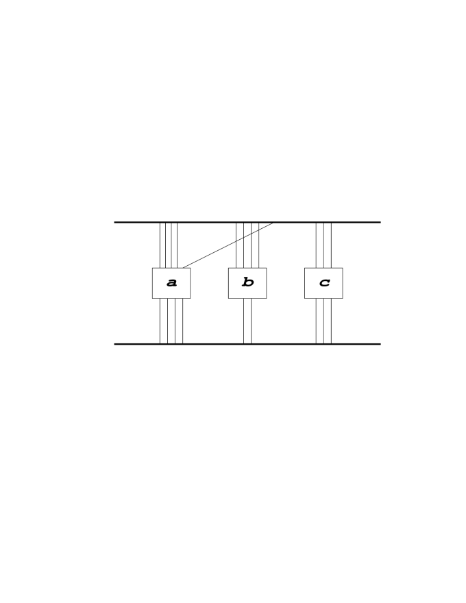
FIG. 4.: A crossed Feynman diagram with three irreducible components.

FIG. 5.: An uncrossed cut diagram with three irreducible components.

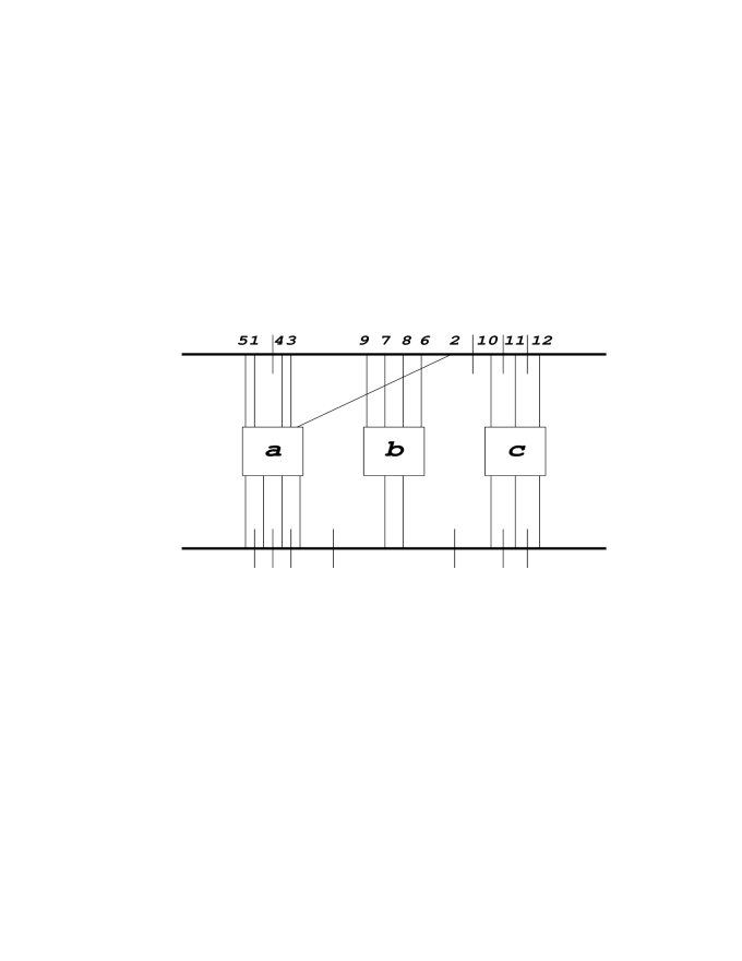
FIG. 6.: A crossed cut diagram with two irreducible components.

FIG. 7.: Two uncrossed cut diagrams differing from each other by the permutation of the first two components. The thick lines are Reggeon fragments.

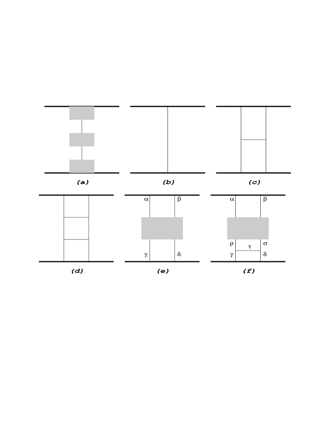
FIG. 8.: Various colour diagrams referred to in the text and in Appendix A.

FIG. 9.: $\gamma^{*}P$ total cross section as a function of photon virtuality $Q^{2}$ and c.m. energy $\sqrt{s}$. The solid curve is a fit of the three-loop eq. (38), with $\Lambda(Q)=[0.2+4Q]GeV$ and $\mu(Q)$ chosen arbitrarily. The dotted and the dashed curves represent an $s^{0.08}$ and an $s^{0.5}$ variation respectively. Data are taken from Ref. [2].

FIG. 10.: The universal energy variation curve $f(s^{\prime})$ obtained from the three-loop formula (38), with arbitrary normalizations. The data are those of Fig. 6, with the same $\Lambda(Q)$, but with all low energy points with $s<1000(GeV)^{2}$ removed.

REFERENCES

- [1] H1 Collaboration, hep-ex/9708016; ZEUS Collaboration, hep-ex/9809005, 9709021, 9602010.
- [2] ZEUS Collaboration, hep-ex/9707025.
- [3] For a review, see V. Del Duca, hep-ph/9503226; L.N. Lipatov, Phys. Reports 286 (1997) 131; E. Levin, hep-ph/9808486.
- [4] L.N. Lipatov, Yad. Fiz. 23 (1976) 642 [Sov. J. Nucl. Phys. 23 (1976) 338]; Ya. Ya. Balitskii and L.N. Lipatov, Yad. Fiz. 28 (1978) 1597 [Sov. J. Nucl. Phys. 28 (1978) 822]; E.A. Kuraev, L.N. Lipatov, and V.S. Fadin, Zh. Eksp. Teor. Fiz. 71 (1976) 840 [Sov. Phys. JETP 44 (1976) 443]; ibid. 72 (1977) 377 [ibid. 45 (1977) 199].
- [5] V.S. Fadin and L.N. Lipatov, Nucl. Phys. B477 (1996) 767, Phys. Lett. B429 (1998) 127; E. Levin, hep-ph/9806228; C.R. Schmidt, hep-ph/9901397; H.-N. Li, hep-ph/9806211; Y.V. Kovchegov and A.H. Mueller, hep-ph/9805208.
- [6] A.H. Mueller, Nucl. Phys. B307 (1988) 34, B317 (1989) 573, B335 (1990) 115; Y.V. Kovchegov, A.H. Mueller, and S. Wallon, hep-ph/9704369.
- [7] J.J. Sakurai, Modern Quantum Mechanics, (Addison-Wesley, 1994).
- [8] R. Torgerson, Phys. Rev. 143 (1966) 1194; H. Cheng and T.T. Wu, Phys. Rev. 182 (1969) 1868, 1899; M. Levy and J. Sucher, Phys. Rev. 186 (1969) 1656.
- [9] G. Sterman, An Introduction to Quantum Field Theory’, (Cambridge University Press, 1993).
- [10] H. Cheng and T.T. Wu, ‘Expanding Protons: Scattering at High Energies’, (M.I.T. Press, 1987).
- [11] L.V. Gribov, E.M. Levin, and M.G. Ryskin, Phys. Reports 100 (1983) 1.
- [12] L.N. Lipatov, hep-ph/950208; E. Verlinde and H. Verlinde, hep-th/9302104.
- [13] H. Cheng and T.T. Wu, Phys. Rev. Lett. 24 (1970) 1456.
- [14] C.S. Lam, Chinese J. of Phys. 35 (1997) 758.
- [15] C.S. Lam and K.F. Liu, Nucl. Phys. B483 (1997) 514.
- [16] C.S. Lam, J. Math. Phys. 39 (1998) 5543.
- [17] Y.J. Feng, O. Hamidi-Ravari, and C.S. Lam, Phys. Rev. D 54 (1996) 3114.
- [18] Y.J. Feng and C.S. Lam, Phys. Rev. D 55 (1997) 4016.
- [19] H. Cheng, J.A. Dickinson, and K. Olaussen, Phys. Rev. D 23 (1981) 534.
- [20] A. Donnachie and P.V. Landshoff, Phys. Lett. B296 (1992) 227.
- [21] C.S. Lam, hep-ph/9808417.