E. Marco^1,2, S. Hirenzaki³, E. Oset^1,2 and H. Toki¹

Abstract

We study the $\rho^{0}$ and $\phi$ decays into $\pi^{+}\pi^{-}\gamma$, $\pi^{0}\pi^{0}\gamma$ and $\phi$ into $\pi^{0}\eta\gamma$ using a chiral unitary approach to deal with the final state interaction of the $MM$ system. The final state interaction modifies only moderately the large momenta tail of the photon spectrum of the $\rho^{0}\rightarrow\pi^{+}\pi^{-}\gamma$ decay. In the case of $\phi$ decay the contribution to $\pi^{+}\pi^{-}\gamma$ and $\pi^{0}\pi^{0}\gamma$ decay proceeds via kaonic loops and gives a distribution of $\pi\pi$ invariant masses in which the $f_{0}(980)$ resonance shows up with a very distinct peak. The spectrum found for $\phi\rightarrow\pi^{0}\pi^{0}\gamma$ decay agrees with the recent experimental results obtained at Novosibirsk. The branching ratio for $\phi\rightarrow\pi^{0}\eta\gamma$, dominated by the $a_{0}(980)$, is also in agreement with recent Novosibirsk results.

PACS: 13.25.Jx 12.39.Fe 13.40.Hq

In this work we investigate the reactions $\rho\rightarrow\pi^{+}\pi^{-}\gamma$, $\pi^{0}\pi^{0}\gamma$ and $\phi\rightarrow\pi^{+}\pi^{-}\gamma$, $\pi^{0}\pi^{0}\gamma$, $\pi^{0}\eta\gamma$, treating the final state interaction of the two mesons with techniques of chiral unitary theory recently developed. The energies of the two meson system are too big in both the $\rho$ and $\phi$ decay to be treated with standard chiral perturbation theory, $\chi PT$ [1]. However, a unitary coupled channels method, which makes use of the standard chiral Lagrangians together with an expansion of Re $T^{-1}$ instead of the $T$ matrix, has proved to be very efficient in describing the meson meson interactions in all channels up to energies around 1.2 GeV [2, 3, 4]. The method is analogous to the effective range expansion in Quantum Mechanics. The work of [4] establishes a direct connection with $\chi PT$ at low energies and gives the same numerical results as the work of [3] where tadpoles and loops in the crossed channels are not evaluated but are reabsorbed into the $L_{i}$ coefficients of the second order Lagrangian of $\chi PT$. A technically much simpler approach is done in [2] where, only for $L=0$, it is shown that the effect of the second order Lagrangian can be suitably incorporated by means of the Bethe-Salpeter equation using the lowest order Lagrangian as a source of the potential and a suitable cut off, of the order of 1 GeV, to regularize the loops. This latter approach will be the one used here, where the two pions interact in s-wave.

The diagrammatic description for the $\rho\rightarrow\pi^{+}\pi^{-}\gamma$ decay is shown in Fig. 1

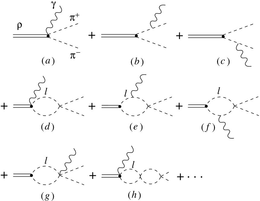
Figure 1: Diagrams for the decay $\rho\rightarrow\pi^{+}\pi^{-}\gamma$.

In Fig. 1 the intermediate states in the loops attached to the photon, $l$, can be $K^{+}K^{-}$ or $\pi^{+}\pi^{-}$. However, the other loops involving only the meson meson interaction can be also $K^{0}\bar{K}^{0}$ or $\pi^{0}\pi^{0}$ in the coupled channel approach of [2].

For the case of $\pi^{0}\pi^{0}\gamma$ decay only the diagrams with at least one loop contribute, $(d),(e),(f),(g),(h),\ldots$ in Fig. 1.

The case of the $\phi$ decay is analogous to the $\rho\rightarrow\pi^{0}\pi^{0}\gamma$ decay. Indeed, the terms $(a),(b),(c)$ of Fig. 1 do not contribute since we do not have direct $\phi\rightarrow\pi\pi$ coupling. Furthermore, there is another novelty since only $K^{+}K^{-}$ contributes to the loop with a photon attached.

The procedure followed here in the cases of $\pi^{0}\pi^{0}$ and $\pi^{0}\eta$ production is analogous to the one used in [5]. Depending on the renormalization scheme chosen, other diagrams can appear [5] but the whole set is calculated using gauge invariant arguments, as done here, with the same result. The novelty in the present work is that the strong interaction $MM\rightarrow M^{\prime}M^{\prime}$ is evaluated using the unitary chiral amplitudes instead of the lowest order used in [5].

We shall make use of the chiral Lagrangians for vector mesons of [6] and follow the lines of ref. [7] in the treatment of the radiative rho decay. The Lagrangian coupling vector mesons to pseudoscalar mesons and photons is given by

$${\cal L}_{2}[V(1^{--})]=\frac{F_{V}}{2\sqrt{2}}\langle V_{\mu\nu}f^{\mu\nu}_{+}\rangle+\frac{iG_{V}}{\sqrt{2}}\langle V_{\mu\nu}u^{\mu}u^{\nu}\rangle$$ (1)

where $V_{\mu\nu}$ is a $3\times 3$ matrix of antisymmetric tensor fields representing the octet of vector mesons, $K^{*}$, $\rho$, $\omega_{8}$. All magnitudes involved in Eq. (1) are defined in [6]. The coupling $G_{V}$ is deduced from the $\rho\rightarrow\pi^{+}\pi^{-}$ decay and the $F_{V}$ coupling from $\rho\rightarrow e^{+}e^{-}$. We take the values chosen in [7], $G_{V}=67$ MeV, $F_{V}=153$ MeV. The $\phi$ meson is introduced in the scheme by means of a singlet, $\omega_{1}$, going from SU(3) to U(3) through the substitution $V_{\mu\nu}\rightarrow V_{\mu\nu}+I_{3}\frac{\omega_{1,\mu\nu}}{\sqrt{3}}$, with $I_{3}$ the $3\times 3$ diagonal matrix. Then, assuming ideal mixing for the $\phi$ and $\omega$ mesons

$$\sqrt{\frac{2}{3}}\omega_{1}+\frac{1}{\sqrt{3}}\omega_{8} \equiv \omega$$

$$\frac{1}{\sqrt{3}}\omega_{1}-\frac{2}{\sqrt{6}}\omega_{8} \equiv \phi$$ (2)

one obtains the Lagrangian of Eq. (1) substituting $V_{\mu\nu}$ by $\tilde{V}_{\mu\nu}$, given by

$$\tilde{V}_{\mu\nu}\equiv\left(\begin{array}[]{ccc}\frac{1}{\sqrt{2}}\rho^{0}_{\mu\nu}+\frac{1}{\sqrt{2}}\omega_{\mu\nu}&\rho^{+}_{\mu\nu}&K^{*+}_{\mu\nu}\\ \rho^{-}_{\mu\nu}&-\frac{1}{\sqrt{2}}\rho^{0}_{\mu\nu}+\frac{1}{\sqrt{2}}\omega_{\mu\nu}&K^{*0}_{\mu\nu}\\ K^{*-}_{\mu\nu}&\bar{K}^{*0}_{\mu\nu}&\phi_{\mu\nu}\end{array}\right)$$ (3)

From there one can obtain the couplings corresponding to $VPP$ ($V$ vector and $P$ pseudoscalar) and $VPP\gamma$ with the $G_{V}$ term or the $VPP\gamma$ with the $F_{V}$ term.

The basic couplings needed to evaluate the diagrams of Fig. 1 are

$$t_{\rho\pi^{+}\pi^{-}} = -\frac{G_{V}M_{\rho}}{f^{2}}(p_{\mu}-p^{\prime}_{\mu})\epsilon^{\mu}(\rho)$$

$$t_{\rho\gamma\pi^{+}\pi^{-}} = 2e\frac{G_{V}M_{\rho}}{f^{2}}\epsilon_{\nu}(\rho)\epsilon^{\nu}(\gamma)$$ (4)

$$+\frac{2e}{M_{\rho}f^{2}}\left(\frac{F_{V}}{2}-G_{V}\right)P_{\mu}\epsilon_{\nu}(\rho)[k^{\mu}\epsilon^{\nu}(\gamma)-k^{\nu}\epsilon^{\mu}(\gamma)]$$

$$t_{\gamma\pi^{+}\pi^{-}} = 2ep_{\mu}\epsilon^{\mu}(\gamma)$$

with $p_{\mu}$, $p^{\prime}_{\mu}$ the $\pi^{+},\pi^{-}$ momenta, $P_{\mu}$, $k_{\mu}$ the $\rho$ and photon momenta and $f$ the pion decay constant which we take as $f_{\pi}=93$ MeV.

The vertices of Eq. (4) are easily generalized to the case of $K^{+}K^{-}$. Using the Lagrangian of Eq. (1), in the first two couplings one has an extra factor $1/2$ and the last coupling is the same. The couplings for $\phi K^{+}K^{-}$ and $\phi\gamma K^{+}K^{-}$ which are needed for the $\phi$ decay are like the two first couplings of Eq. (4) substituting $M_{\rho}$ by $M_{\phi}$, $\epsilon^{\mu}(\rho)$ by $\epsilon^{\mu}(\phi)$ and multiplying by $-1/\sqrt{2}$. In addition we shall take the values $G_{V}=55$ MeV and $F_{V}=165$ MeV which are suited to the $\phi\rightarrow K^{+}K^{-}$ and $\phi\rightarrow e^{+}e^{-}$ decay widths respectively.

The evaluation of the $\rho$ width for the first three diagrams $(a),(b),(c)$ of Fig. 1 is straightforward and has been done before [9, 10, 11] and in [7] following the present formalism. We rewrite the results in a convenient way for our purposes

$$\frac{d\Gamma_{\rho}}{dM_{I}} = \frac{1}{(2\pi)^{3}}\frac{1}{16m_{\rho}^{3}}(m_{\rho}^{2}-M_{I}^{2})(M_{I}^{2}-4m_{\pi}^{2})^{1/2}$$ (5)

$$\times\frac{1}{2}\int_{-1}^{1}d\cos\theta\bar{\sum}\sum|t|^{2}$$

where

$$\bar{\sum}\sum|t|^{2}=\frac{8}{3}e^{2}\left[I_{1}+I_{2}+I_{3}\right]$$ (6)

In Eq. (5), $M_{I}$ is the invariant mass of the two $\pi$ system and $\theta$ the angle between the $\pi^{+}$ meson and the photon in the frame where the $\pi^{+}\pi^{-}$ system is at rest. The quantity $I_{1}$ stands for the contribution of the first diagram alone, Fig. 1 $(a)$, $I_{3}$ for the second and third $(b),(c)$ and $I_{2}$ for the interference between the first diagram and the other two. They are given by

$$I_{1} = \left|\frac{M_{\rho}G_{V}}{f^{2}}+\frac{K}{f^{2}}\left(\frac{F_{V}}{2}-G_{V}\right)\right|^{2}$$

$$I_{2} = 2\frac{M_{\rho}G_{V}}{f^{2}}\vec{p}\,^{2}(D_{1}+D_{2})\sin^{2}\theta\left\{\frac{M_{\rho}G_{V}}{f^{2}}+\frac{K}{f^{2}}\left(\frac{F_{V}}{2}-G_{V}\right)\right\}$$

$$I_{3} = 2\vec{p}\,^{2}(D_{1}+D_{2})\sin^{2}\theta$$ (7)

$$\times\left\{(D_{1}+D_{2})\vec{p}\,^{2}+(D_{1}-D_{2})|\vec{p}||\vec{k}|\cos\theta\right\}\left(\frac{M_{\rho}G_{V}}{f^{2}}\right)^{2}$$

where $K$ is the photon momentum in the $\rho$ rest frame and $p,k$ are the momenta of the meson and the photon in the rest frame of the $\pi^{+}\pi^{-}$ system, and $D_{1},D_{2}$ the meson propagators in the $(b),(c)$ Bremsstrahlung diagrams, conveniently written in terms of $M_{I}$ and $\theta$.

The first term of the contact term, $t_{\rho\gamma\pi^{+}\pi^{-}}$, in Eq. (4) is not gauge invariant. It requires the addition of the diagrams $(b)$ and $(c)$ of Fig. 1 to have a gauge invariant set. On the other hand the second term in the contact term ($F_{V}/2-G_{V}$ part) is gauge invariant by itself. When considering final state interaction of the mesons this means that the $G_{V}$ part of the contact term, diagram $(d)$, must be complemented by diagrams $(e)$, $(f)$, $(g)$ to form the gauge invariant set. On the other hand the $F_{V}/2-G_{V}$ part of the contact term appears in the $(d)$ diagram which is gauge invariant by itself.

The technology to introduce the final state interactions is available from the study of $\phi\rightarrow K^{0}\bar{K}^{0}\gamma$ in [12]. There it was shown that the strong $t$ matrix for the $M_{1}M_{2}\rightarrow M^{\prime}_{1}M^{\prime}_{2}$ transition factorizes with their on shell values in the loops with a photon attached. The same was proved for the loops of the Bethe-Salpeter equation in the meson meson interaction description of [2]. On the other hand the sum of the diagrams $(d),(e),(f),(g)$, which appears now with the $G_{V}$ part of the contact term (diagram $(a)$), could be done using arguments of gauge invariance which led to a finite contribution for the sum of the loops [5, 13, 14]. A sketch of the procedure is given here. The $\rho\rightarrow\pi^{+}\pi^{-}\gamma$ amplitude can be written as $\epsilon_{\mu}(\rho)\epsilon_{\nu}(\gamma)T^{\mu\nu}$ and the structure of the loops in Fig. 1 is such that

$$T^{\mu\nu}=a\,g^{\mu\nu}+b\,Q^{\mu}Q^{\nu}+c\,Q^{\mu}K^{\nu}+d\,Q^{\nu}K^{\mu}+e\,K^{\mu}K^{\nu}$$ (8)

where $Q$, $K$ are the $\rho$ meson and photon momenta respectively. Gauge invariance $(T^{\mu\nu}K_{\nu}=0)$ forces $b=0$ and $d=-a/(Q\cdot K)$. Furthermore, in the Coulomb gauge only the $g^{\mu\nu}$ term of Eq.(8) contributes and the coefficient $a$ is calculated from the $d$ coefficient, to which only the diagrams $(e)$, $(f)$, of Fig. 1 contribute. For dimensional reasons the loop integral contains two powers less in the internal variables than the pieces contributing to the $g^{\mu\nu}$ term from these diagrams, since the product $Q^{\nu}K^{\mu}$ is factorized out of the integral. This makes the $d$ coefficient finite. Furthermore, the $MM\rightarrow MM$ vertices appearing there have the structure $\alpha s+\beta\sum_{i}p_{i}^{2}+\gamma\sum_{i}m_{i}^{2}$, which can be recast as $\alpha s+(\beta+\gamma)\sum_{i}m_{i}^{2}+\beta\sum_{i}(p_{i}^{2}-m_{i}^{2})$. The first two terms in the sum give the on shell contribution and the third one the off shell part. This latter term kills one of the meson propagators in the loops and does not contribute to the $d$ term in Eq. (8). Hence, the meson meson amplitudes factorize outside the loop integral with their on shell values. A more detailed description, done for a similar problem, can be seen in [15], following the steps from Eqs. (13) to (23).

Following these steps, as done in [12, 15], it is easy to include the effect of the final state interaction of the mesons. The sum of the diagrams $(d),(e),(f),(g)$ and further iterated loops of the meson-meson interaction, $(h),\ldots,$ is shown to have the same structure as the contact term of $(a)$ in the Coulomb gauge, which one chooses to evaluate the amplitudes. The sum of all terms including loops is readily accomplished by multiplying the $G_{V}$ part of the contact term by the factor $F_{1}(M_{\rho},M_{I})$

$$F_{1}(M_{\rho},M_{I})=1+\tilde{G}_{\pi^{+}\pi^{-}}t_{\pi^{+}\pi^{-},\pi^{+}\pi^{-}}+\frac{1}{2}\tilde{G}_{K^{+}K^{-}}t_{K^{+}K^{-},\pi^{+}\pi^{-}}$$ (9)

where $t_{M_{1}M_{2},M^{\prime}_{1}M^{\prime}_{2}}$ are the strong transition matrix elements in s-wave evaluated in [2] and $\tilde{G}_{M_{1}M_{2}}$ is given by

$$\tilde{G}_{M_{1}M_{2}}(M_{\rho},M_{I})=\frac{1}{8\pi^{2}}(a-b)I(a,b)$$

$$a=\frac{M_{\rho}^{2}}{M_{M_{1}}^{2}};\quad b=\frac{M_{I}^{2}}{M_{M_{1}}^{2}}$$ (10)

with $I(a,b)$ a function given analytically in [12]. The $({F_{V}}/{2}-G_{V})$ part of the contact term is iterated by means of diagrams $(d)$, $(h)\ldots$ in order to account for final state interaction. Here the loop function is the ordinary two meson propagator function, $G$, of the Bethe-Salpeter equation, $T=V+VGT$, for the meson-meson scattering and which is regularized in [2] by means of a cut-off in order to fit the scattering data. The sum of all these diagrams is readily accomplished by multiplying the $({F_{V}}/{2}-G_{V})$ part of the contact term by the factor

$$F_{2}(M_{I})=1+G_{\pi^{+}\pi^{-}}t_{\pi^{+}\pi^{-},\pi^{+}\pi^{-}}+\frac{1}{2}G_{K^{+}K^{-}}t_{K^{+}K^{-},\pi^{+}\pi^{-}}$$ (11)

By using isospin Clebsch Gordan coefficients the amplitudes $t_{M_{1}M_{2},M^{\prime}_{1}M^{\prime}_{2}}$ can be written in terms of the isospin amplitudes of [2] as

$$t_{\pi^{+}\pi^{-},\pi^{+}\pi^{-}} = \frac{2}{3}t_{\pi\pi,\pi\pi}^{I=0}(M_{I})$$

$$t_{K^{+}K^{-},\pi^{+}\pi^{-}} = \frac{1}{\sqrt{3}}t_{K\bar{K},\pi\pi}^{I=0}(M_{I})$$ (12)

neglecting the small $I=2$ amplitudes. In Eq. (S0.Ex10), one factor $\sqrt{2}$ for each $\pi^{+}\pi^{-}$ state has been introduced, since the isospin amplitudes of [2] used in Eq. (S0.Ex10) are written in a unitary normalization which includes an extra factor $1/\sqrt{2}$ for each $\pi\pi$ state.

The invariant mass distribution in the presence of final state interaction is now given by Eqs. (5, 6, S0.Ex6) by changing in Eq. (S0.Ex6)

$$I_{1} \rightarrow \left|\frac{M_{\rho}G_{V}}{f^{2}}F_{1}(M_{\rho},M_{I})+\frac{K}{f^{2}}\left(\frac{F_{V}}{2}-G_{V}\right)F_{2}(M_{I})\right|^{2}$$

$$I_{2} \rightarrow 2\frac{M_{\rho}G_{V}}{f^{2}}\vec{p}\,^{2}(D_{1}+D_{2})\sin^{2}\theta$$

$$\times\mbox{Re}\left\{\frac{M_{\rho}G_{V}}{f^{2}}F_{1}(M_{\rho},M_{I})+\frac{K}{f^{2}}(\frac{F_{V}}{2}-G_{V})F_{2}(M_{I})\right\}$$

$$I_{3} \rightarrow I_{3}$$ (13)

The $\rho\rightarrow\pi^{0}\pi^{0}\gamma$ width is readily obtained by omitting the terms $I_{2},I_{3}$ and also omitting the first term (the unity) in the definition of the $F_{1}(M_{\rho},M_{I})$, $F_{2}(M_{I})$ factors in Eqs. (9) and (11) and dividing by a factor two the width to account for the identity of the particles.

The evaluation of the $\phi$ decay is straightforward by noting that the tree level contributions, diagrams $(a),(b),(c)$ are not present now, and that only kaonic loops attached to photons contribute in this case. Hence, the invariant mass distribution for $\phi\rightarrow\pi^{+}\pi^{-}\gamma$ is given in this case by Eq. (5), changing $m_{\rho}\rightarrow m_{\phi}$, with

$$\bar{\sum}\sum|t|^{2}=\frac{4}{3}e^{2}\left|\frac{M_{\phi}G_{V}}{f^{2}}\frac{1}{\sqrt{3}}\tilde{G}_{K^{+}K^{-}}t_{K\bar{K},\pi\pi}^{I=0}+\frac{K}{f^{2}}\left(\frac{F_{V}}{2}-G_{V}\right)\frac{1}{\sqrt{3}}G_{K^{+}K^{-}}t_{K\bar{K},\pi\pi}^{I=0}\right|^{2}$$ (14)

For $\phi\rightarrow\pi^{0}\pi^{0}\gamma$ the cross section is the same divided by a factor two to account fot the identity of the two $\pi^{0}$’s.

For the $\phi\rightarrow\pi^{0}\eta\gamma$ case we have

$$\bar{\sum}\sum|t|^{2}=\frac{4}{3}e^{2}\left|\frac{M_{\phi}G_{V}}{f^{2}}\frac{1}{\sqrt{2}}\tilde{G}_{K^{+}K^{-}}t_{K\bar{K},\pi\eta}^{I=1}+\frac{K}{f^{2}}\left(\frac{F_{V}}{2}-G_{V}\right)\frac{1}{\sqrt{2}}\tilde{G}_{K^{+}K^{-}}t_{K\bar{K},\pi\eta}^{I=1}\right|^{2}$$ (15)

Figure 2: Photon distribution, $d\Gamma/dK$, for the process $\rho\rightarrow\pi^{+}\pi^{-}\gamma$ as a function of the photon momentum. Solid line: spectrum including final state interaction of the two mesons and the $F_{V}$ and $G_{V}$ contributions; dashed line: spectrum including only the tree level diagrams $(a),(b),(c)$ of Fig. 1 and the $F_{V}$ and $G_{V}$ contributions; dashed-dotted line: spectrum including only the tree level diagrams $(a),(b),(c)$ of Fig. 1 and taking $F_{V}=0$. The experimental data taken from [16] are normalized to our results.

In Fig. 2 we show $d\Gamma/dK$ for $\rho\rightarrow\pi^{+}\pi^{-}\gamma$ decay, $(d\Gamma_{\rho}/dK=m_{\rho}d\Gamma_{\rho}/M_{I}dM_{I})$. The dashed-dotted line shows the contribution of diagrams $1(a),(b),(c)$ and taking $F_{V}=0$. The dashed line shows again the contribution coming from diagrams $1(a),(b),(c)$ but now considering also the $F_{V}$ contributions. Finally, the solid line includes the full set of diagrams in Fig. 1 to account for final state interaction and with the $F_{V}$ and $G_{V}$ contributions. The process is infrared divergent and we plot the distribution for photons with energy bigger than 50 MeV, where the experimental measurements exist [16]. We have also added the experimental data, given in [16] with arbitrary normalization, normalized to our results.

As one can see in Fig. 2, the shape of the distribution of photon momenta is well reproduced. For the total contribution we obtain a branching ratio to the total width of the $\rho$

$$B(\rho^{0}\rightarrow\pi^{+}\pi^{-}\gamma)=1.18\,\,10^{-2}\quad\mbox{for $K>50$ MeV}$$ (16)

which compares favourably with the experimental number [16], $B^{\mbox{\scriptsize exp}}(\rho^{0}\rightarrow\pi^{+}\pi^{-}\gamma)=(0.99\pm 0.04\pm 0.15)\,\,10^{-2}$ for $K>50$ MeV.

The changes induced by the $F_{V}$ term found here reconfirm the findings of [7]. The effect of the final state interaction is small and mostly visible at high photon energies, where it increases $d\Gamma/dK$ by about 25%. The branching ratio for $B(\rho^{0}\rightarrow\pi^{0}\pi^{0}\gamma)$ that we obtain is $1.4\,\,10^{-5}$ which can be interpreted in our case as $\rho^{0}\rightarrow\gamma\sigma(\pi^{0}\pi^{0})$ since the $\pi^{0}\pi^{0}$ interaction is dominated by the $\sigma$ pole in the energy regime where it appears here. This result is very similar to the one obtained in [5]. In the case one considers $F_{V}G_{V}<0$, the result obtained is $1.0\,\,10^{-4}$. The measurement of this quantity may serve as a test for the sign of the $F_{V}G_{V}$ product.

Figure 3: Distribution $dB/dM_{I}$ for the decay $\phi\rightarrow\pi^{0}\pi^{0}\gamma$, with $M_{I}$ the invariant mass of the $\pi^{0}\pi^{0}$ system. Solid line: our prediction, with $F_{V}G_{V}>0$. Dashed line: result taking $F_{V}G_{V}<0$. The data points are from [17] and only statistical errors are shown. The systematic errors are similar to the statistical ones [17]. The distribution for $\phi\rightarrow\pi^{+}\pi^{-}\gamma$ is twice the results plotted there.

As for the $\phi\rightarrow\pi\pi\gamma$ decay, as we pointed above the $\phi\rightarrow\pi^{+}\pi^{-}\gamma$ rate is twice the one of the $\phi\rightarrow\pi^{0}\pi^{0}\gamma$. We have evaluated the invariant mass distribution for these decay channels and in Fig. 3 we plot the distribution $dB/dM_{I}$ for $\phi\rightarrow\pi^{0}\pi^{0}\gamma$ which allows us to see the $\phi\rightarrow f_{0}\gamma$ contribution since the $f_{0}$ is the important scalar resonance appearing in the $K^{+}K^{-}\rightarrow\pi^{+}\pi^{-}$ amplitude [2]. The solid curve shows our prediction, with $F_{V}G_{V}>0$, the sign predicted by vector meson dominance [6]. The dashed curve is obtained considering $F_{V}G_{V}<0$. We compare our results with the recent ones of the Novosibirsk experiment [17]. We can see that the shape of the spectrum is relatively well reproduced considering statistical and systematic errors (the latter ones not shown in the figure). The results considering $F_{V}G_{V}<0$ are in complete disagreement with the data.

The finite total branching ratio which we find for $\phi\rightarrow\pi^{+}\pi^{-}\gamma$ is $1.6\,\,10^{-4}$ and correspondingly $0.8\,\,10^{-4}$ for the $\phi\rightarrow\pi^{0}\pi^{0}\gamma$. This latter number is slightly smaller than the result given in [17], $(1.14\pm 0.10\pm 0.12)\,\,10^{-4}$, where the first error is statistical and the second one systematic. The result given in [18] is $(1.08\pm 0.17\pm 0.09)\,\,10^{-4}$, compatible with our prediction. The branching ratio measured in [20] for $\phi\rightarrow\pi^{+}\pi^{-}\gamma$ is $(0.41\pm 0.12\pm 0.04)\,\,10^{-4}$.

The branching ratio obtained for the case $\phi\rightarrow\pi^{0}\eta\gamma$ is $0.87\,\,10^{-4}$. The results obtained at Novosibirsk are [19] $(0.83\pm 0.23)\,\,10^{-4}$ and [18] $(0.90\pm 0.24\pm 0.10)\,\,10^{-4}$. The spectrum, not shown, is dominated by the $a_{0}$ contribution.

The contribution of $\phi\rightarrow f_{0}(\pi^{+}\pi^{-})\gamma$, obtained by integrating $d\Gamma_{\phi}/dM_{I}$ assuming an approximate Breit-Wigner form to the left of the $f_{0}$ peak, gives us a branching ratio $0.44\,\,10^{-4}$. As argued above, the branching ratio for $\phi\rightarrow\pi^{0}\pi^{0}\gamma$ is one half of $\phi\rightarrow\pi^{+}\pi^{-}\gamma$, which should not be compared to the one given in [17] since there the assumption that all the strength of the spectrum is due to the $f_{0}$ excitation is done. As one can see in Fig. 3, we find also an appreciable strength for $\phi\rightarrow\sigma\gamma$.

We should also warn not to compare our predicted rate for $\phi\rightarrow\pi^{+}\pi^{-}\gamma$ directly with experiment. Indeed, the experiment is done using the reaction $e^{+}e^{-}\rightarrow\phi\rightarrow\pi^{+}\pi^{-}\gamma$, which interferes with the $\rho$ contribution $e^{+}e^{-}\rightarrow\rho\rightarrow\pi^{+}\pi^{-}\gamma$ at the tail of the $\rho$ mass distribution in the $\phi$ mass region [21]. Also the results in [18, 20] are based on model dependent assumptions. For these reasons, as quoted in [18], the $\pi^{0}\pi^{0}\gamma$ mode is more efficient to study the $\pi\pi$ mass spectrum.

Our result for $\phi\rightarrow\pi^{0}\pi^{0}\gamma$ is 50 % larger than the one obtained in [5] owed to the use of the unitary $K^{+}K^{-}\rightarrow\pi^{0}\pi^{0}$ amplitude instead of the lowest order chiral one. The shape of the distribution found here is, however, rather different than the one obtained in [5], showing the important contribution of the $f_{0}$ resonance which appears naturally in the unitary chiral approach.

The $\phi\rightarrow f_{0}\gamma$ decay has been advocated as an important source of information on the nature of the $f_{0}$ resonance and experiments have been conducted at Novosibirsk [22] and are also planned at Frascati [23], trying to magnify the signal for $f_{0}$ production through interference with initial and final state radiation in the $e^{+}e^{-}\rightarrow\phi\rightarrow f_{0}(\pi^{+}\pi^{-})\gamma$ reaction [21, 23, 24, 25]. The completion of the experiments [17, 18, 19, 20] is a significant step forward.

Present evaluations for $\phi\rightarrow f_{0}\gamma\rightarrow\pi\pi\gamma$ are based on models assuming a $K\bar{K}$ molecule for the $f_{0}$ [26] with a branching ratio 1-$2\,\,10^{-5}$, a $q\bar{q}$ structure with a value $5\,\,10^{-5}$ [26] and a $q\bar{q}q\bar{q}$ structure with a value $2.4\,\,10^{-4}$ [26].

The model for $\phi\rightarrow f_{0}\gamma$ assumed in Fig. 1 is similar to the one of [27] where the production also proceeds via the kaonic loops. There a $K\bar{K}$ molecule is assumed for the $f_{0}$ resonance while here the realistic $K\bar{K}\rightarrow\pi\pi$ amplitude of [2] is used. Emphasis is made in the importance of going beyond the zero width approximation for the resonance in [27, 28]. Our approach automatically takes this into account since the $K\bar{K}\rightarrow\pi\pi$ amplitude correctly incorporates the width of the $f_{0}$ resonance [2].

We would also like to warn that the peak of the $f_{0}$ seen in Fig. 3 cannot be trivially interpreted as a resonant contribution on top of a background, since there are important interference effects between the $f_{0}$ production and the $\sigma$ background. The strength of the peak comes in our case in about equal amounts from the real and the imaginary parts of the amplitude for the process.

The agreement found between our results for the $\phi\rightarrow\pi^{0}\pi^{0}\gamma$, $\phi\rightarrow\pi^{0}\eta\gamma$ and experiment provides an important endorsement for the chiral unitary approach used here. Improvements in the future, reducing the experimental errors, should put further constraints on avalaible theoretical approaches for this reaction.

Acknowledgments:

We would like to acknowledge useful comments from J. A. Oller and from A. Bramon who called our attention to the recent experimental results on $\phi\rightarrow\pi^{0}\pi^{0}\gamma$. We are grateful to the COE Professorship program of Monbusho which enabled E.O. to stay at RCNP to perform the present study. One of us, E.M., wishes to thank the hospitality of the RCNP of the University of Osaka, and acknowledges finantial support from the Ministerio de Educación y Cultura. This work is partly supported by DGICYT contract no. PB 96-0753 and by the EEC-TMR Program Contract No. ERBFMRX-CT98-0169.

References

[1] J. Gasser and H. Leutwyler, Nucl. Phys. B 250
(1985) 465, 517, 539.
[2] J.A. Oller and E. Oset, Nucl. Phys. A620 (1997) 438;
erratum Nucl. Phys. A 624 (1999) 407.
[3]
J.A. Oller, E. Oset and J. R. Peláez, Phys. Rev. Lett. 80 (1998) 3452;
ibid, Phys. Rev. D 59 (1999) 74001.
[4] F. Guerrero and J.A. Oller, Nucl. Phys. B 537 (1999) 459.
[5] A. Bramon, A. Grau and G. Pancheri, Phys. Lett. B 289 (1992) 97.
[6] G. Ecker, J. Gasser, A. Pich and E. de Rafael, Nucl. Phys. B
321 (1989) 311.
[7] K. Huber and H. Neufeld, Phys. Lett. B 357 (1995) 221.